No FIP fractionation in the active stars AR Psc and AY Cet

Abstract

Context. The comparison of coronal and photospheric abundances in cool stars is an essential question to resolve. In the Sun an enhancement of the elements with low first ionization potential (FIP) is observed in the corona with respect to the photosphere. Stars with high levels of activity seem to show a depletion of elements with low FIP when compared to solar standard values; however, the few cases of active stars in which photospheric values are available for comparison lead to confusing results, and an enlargement of the sample is mandatory for solving this longstanding problem.

Aims. We calculate in this paper the photospheric and coronal abundances of two well known active binary systems, AR Psc and AY Cet, to get further insight into the complications of coronal abundances.

Methods. Coronal abundances of 9 elements were calculated by means of the reconstruction of a detailed emission measure distribution, using a line-based method that considers the lines from different elements separately. Photospheric abundances of 8 elements were calculated using high-resolution optical spectra of the stars.

Results. The results once again show a lack of any FIP-related effect in the coronal abundances of the stars. The presence of metal abundance depletion (MAD) or inverse FIP effects in some stars could stem from a mistaken comparison to solar photospheric values or from a deficient calculation of photospheric abundances in fast-rotating stars.

Conclusions. The lack of FIP fractionation seems to confirm that Alfvén waves combined with pondermotive forces are dominant in the corona of active stars.

1 Introduction

One of the most debated issues in stellar astrophysics is whether the coronal abundances are similar to the photospheric counterparts in cool stars. A different composition in the corona and the photosphere would indicate a physical process taking place somewhere between the cooler photospheric material and the hotter corona. Such a process should be capable of distinguishing between different elements based on a certain physical variable. A pattern related to that variable would help understanding the physical processes taking place in the coronal loops. Such a pattern has been observed in the Sun, which shows, on average, an enhancement of elements with a low first ionization potential (FIP) in the corona with respect to the photosphere. The so called “FIP effect” is actually observed in the solar corona and slow wind, but is absent in coronal holes or fast wind (Laming et al., 1995; Feldman & Laming, 2000). Stars similar to the Sun, such as $\alpha$ Cen, show a similar FIP effect (Drake et al., 1997; Raassen et al., 2003). Less active stars, such as Procyon (F4IV), do not show any fractionation (Raassen et al., 2002; Sanz-Forcada et al., 2004). Intermediate-activity stars, like $\epsilon$ Eri, 36 Oph or 70 Oph present a much lower FIP effect, if any is present (Laming et al., 1996; Sanz-Forcada et al., 2004; Wood & Linsky, 2006; Ness & Jordan, 2008).

For the most active stars, the results are more uncertain. Their coronal composition is relatively easy to determine once high spectral resolution is available. But their high rotation rates hamper the measurements of photospheric composition due to line broadening, making the comparison more difficult. The photospheric composition can only be well calculated for stars with low projected rotational velocity ($v\sin i$). Initial studies of active stars made with XMM-Newton and Chandra high-resolution spectra found a very different pattern from the Sun (e.g. Güdel, 2004, and references therein). The elements with low FIP would actually be underabundant in the corona, a “metal abundance depletion” (“MAD syndrome”, Schmitt et al., 1996), or alternatively, the elements with high FIP would be enhanced in the corona (the “inverse FIP effect”, Brinkman et al., 2001). A caveat of many of the active stars is that their coronal abundances are actually compared to the solar photosphere, which at least yields to risky conclusions (Favata & Micela, 2003). Moreover, most active stars with photospheric abundances calculated have large $v\sin i$, with broad photospheric lines. As a result, their abundances determination could actually carry some hidden errors not assessed well by formal calculations. This is the case for II Peg, AB Dor, or AR Lac (see Table 1).

Table 1: Fractionation effects in other stars with known photospheric and coronal abundances

Star	HD	Sp. Type	$L_{\rm X}$	$L_{\rm X}$/$L_{\rm bol}$	$v\sin i$	FIP effect?	Referencea
			(erg s-1)		km s-1
Sun	…	G2V	$\sim$27.5	-6.1	…	FIP effect	FE00
Procyon	61421	F4IV	27.9	-6.5	6.1	No FIP effect	SF04,RA02
$\epsilon$ Eri	22049	K2V	28.2	-5.1	2.4	Small/No FIP effect	SF04
$\xi$ UMa B	98230	G5V/[KV]	29.5	-4.3	2.8	(No FIP effect)	BA05
$\lambda$ And	222107	G8III/?	30.4	-4.5	7.3	No FIP effect	SF04
Capella	34029	G1III/G8III	30.5	-5.3	32.7	(No FIP effect)	BR00
II Peg	224085	K2IV/M0-3V	31.1	-2.8	21	Small inverse FIP	HU01
AB Dor	25647	K1IV	30.1	-3.0	90	Inverse FIP	SF03
AR Lac	210334	G2IV/K0IV	30.9	-3.4	46/81	Small inverse FIP	HU03
V851 Cen	119285	K2IV-III/?	30.8	-3.5	6.5	No FIP effect	SF04
AR Psc	8357	G7V/K1IV	30.7	-3.3	7.0	No FIP effect	This work
AY Cet	7672	WD/G5III	31.0	-4.2	4.6	No FIP effect	This work

Note: $L_{\rm X}$ (erg s^-1) calculated in the range 5–100 Å (0.12–2.4 keV).
^aReferences for FIP effect: BA05 (Ball et al., 2005), BR00 (Brickhouse et al., 2000), FE00 (Feldman & Laming, 2000), HU01 (Huenemoerder et al., 2001), HU03 (Huenemoerder et al., 2003), RA02 (Raassen et al., 2002), SF04 (Sanz-Forcada et al., 2004), SF03 (Sanz-Forcada et al., 2003b).

Figure 1: Light curves of AR Psc (using all EPIC detectors) and AY Cet (using order +1 and -1 of LETGS) in X-rays. Upper axis indicate the orbital phase, assuming that secondary star is located behind the primary star at phase 0.

Theoretical explanations of the FIP effect are found in Laming (2004). The authors also propose that Alfvén waves, combined with pondermotive forces, would explain the observed FIP effect on the Sun, pointing towards the disappearance of any fractionation of stars with lower or higher activity levels. The same mechanism could also explain the inverse FIP effect, if such exists, by reflecting the Alfvén waves in the chromosphere. Alfén waves are also being suggested in recent years as responsible for the energy transportation between the outer convective layers of the star and the much hotter corona (e.g. Erdélyi & Fedun, 2007; De Pontieu et al., 2007, and references therein), one of the most important problems unresolved in stellar astrophysics. Both questions, the energy transportation and the FIP fractionation, could actually be connected.

It is thus essential to understand whether active stars suffer an inverse FIP effect or just no significant fractionation with respect to the photospheric composition. Given the problems measuring the photospheric abundances, we should mainly trust those results for stars with low $v\sin i$. Sanz-Forcada et al. (2004) showed the case of two active stars, $\lambda$ And and V851 Cen, for which coronal and photospheric abundances are consistent, and no effect related to FIP would be present. Stars such as Capella (which shows solar photospheric abundances, Brickhouse et al., 2000; Argiroffi et al., 2003; Audard et al., 2003) show no inverse FIP effect either, although their photospheric abundance is poorly known ([Fe/H]=–0.16, McWilliam, 1990). Other cases of active stars with no sign of an inverse FIP effect, which are compared to poorly known photospheric iron abundances, are $\sigma^{2}$ CrB (Suh et al., 2005), EK Dra (Telleschi et al., 2005), and YY Men (Audard et al., 2004). The present situation is still confusing given the few cases described in the literature with both photospheric and coronal abundances well-calculated. In this work we present the results for two more RS CVn systems known to have narrow photospheric lines despite their high rotation and activity level.

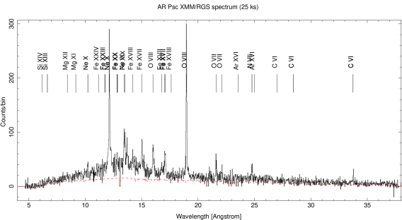
Figure 2: AR Psc and AY Cet X-ray spectra. The dashed line represents the continuum predicted by the EMD.

Following Sanz-Forcada et al. (2004) we have chosen two active stars that are observed with their pole on, and therefore have low $v\sin i$. Thus, their optical spectra display narrow lines, allowing us to measure the photospheric abundances better. The two RS CVn binaries are well known X-ray emitters. Their emission is attributed to coronal activity, powered by the fast rotation forced by the close binariety. AR Psc (G7V/K1IV, $v\sin i$=7 km s^-1, Nordström et al., 2004) and AY Cet (WD/G5III, $v\sin i$=4.6 km s^-1, Massarotti et al., 2008) were observed with the Extreme Ultraviolet Explorer Observatory (EUVE), giving a first glimpse of its coronal emission (Sanz-Forcada et al., 2003a). Optical spectra also indicate a high level of chromospheric activity (Montes et al., 1997). Their EMD is similar to other active stars, either showing an inverse FIP effect, like AB Dor (Sanz-Forcada et al., 2003b; García-Alvarez et al., 2005, 2008), or no FIP-related fractionation, such as $\lambda$ And (Sanz-Forcada et al., 2004). In the case of AY Cet, it is not expected that its white dwarf companion contributes substantially to the X-rays band. Photospheric abundances were calculated by Ottmann et al. (1998) for AY Cet in only three elements: [Fe/H]=-0.32, [Mg/H]=-0.22, and [Si/H]=-0.32, with Asplund et al. (2005) values as reference. Shan et al. (2006) finds a low iron abundance in AR Psc, but no information is provided on the reference system used in the calculations.

The paper is divided as follows: in Sect. 2 the observations are described. Results are given in Sect. 3, with discussion in Sect. 4, to finish with the conclusions.

2 Observations

Time was awarded (P.I. J. Sanz-Forcada) for observing high-resolution X-rays spectra of AY Cet and AR Psc. The Chandra Low Energy Transmission Grating Spectrograph (LETGS) ($\lambda\lambda\sim$3–175, $\lambda/\Delta\lambda\sim$60-1000, Weisskopf et al., 2002) observed AY Cet in May 2005 in combination with the High Resolution Camera (HRC-S). Data were reduced using the CIAO v4.0 package. The positive and negative orders were summed for the flux measurements. Lines formed in the first dispersion order, but contaminated with contribution from higher dispersion orders, were not employed in the analysis. Light curves were obtained from the LETG spectra (first and higher orders) of AY Cet with the background properly subtracted (Fig. 1). XMM-Newton observed AR Psc on 11 January 2006. XMM-Newton observes simultaneously with the RGS (Reflection Grating Spectrometer, den Herder et al., 2001) ($\lambda\lambda\sim$6–38 Å, $\lambda$/$\Delta\lambda\sim$100–500) and the EPIC (European Imaging Photon Camera) PN and MOS detectors (sensitivity range 0.15–15 keV and 0.2–10 keV, respectively). The RGS data were reduced using the standard SAS (Science Analysis Software) version 8.0.1 package, and the RGS 1 and 2 spectra were combined to improve the measurement of the line fluxes (Fig. 2). The EPIC light curve (Fig. 1) was constructed by combining the PN and MOS count rates in a circle around the target, with background regions properly subtracted using the SAS task epiclccorr, which also corrects from several instrumental effects.

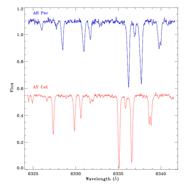
Figure 3: AR Psc and AY Cet optical spectra.

Optical spectra (Fig. 3) were acquired on 27 and 28 November 2002 to calculate the photospheric abundances of the two stars, as part of a wider observational campaign. The detailed instrumental setup and observations are described well in Affer et al. (2005), so only a short description is given here. We used the high-resolution cross-dispersed echelle spectrograph SOFIN, mounted on the Cassegrain focus of the 2.56 m Nordic Optical Telescope (NOT) located at the Observatorio del Roque de Los Muchachos (La Palma, Spain). Exposure times ranged from 4 to 20 min, resulting in high S/N per pixel ($\approx 0.025$ Å/px)  averaging at about 280. A spectrum of a Th-Ar lamp was obtained following each stellar spectrum, ensuring accurate wavelength calibration. The total spectral range is 3900–9900 Å, and the resolving power is $R=\lambda/\Delta\lambda\,\approx\,80\,000$. The spectra were reduced with the standard software available within the CCDRED and ECHELLE packages of IRAF. The analysis includes overscan subtraction, flat-fielding, removal of scattered light, extraction of one-dimensional spectra, wavelength calibration, and continuum normalization (see Affer et al., 2005, for further details). The $EW$s were measured using the SPLOT task in IRAF, assuming a Gaussian profile for weak or moderately strong lines ($EW\la 100$ mÅ) and a Voigt profile for stronger lines. The accuracy (absolute error) is harder to assess. It almost certainly contains a systematic error due to the continuum location, because of the presence of interference fringes (which could not be completely removed) in the redder part of the stellar spectra, which cause a modulation of the local continuum. This error could be particularly important for the weak lines.

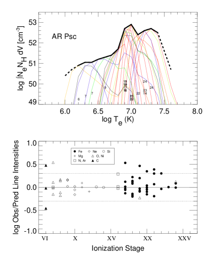
Figure 4: Emission measure distribution (EMD) of AR Psc and AY Cet. Thin lines represent the relative contribution function for each ion (the emissivity function multiplied by the EMD at each point). Small numbers indicate the ionization stages of the species. Also plotted are the observed-to-predicted line flux ratios for the ion stages in the upper figure. The dotted lines denote a factor of 2.

2

Table 2: XMM/RGS line fluxes of AR Psc^a

Ion	$\lambda$model	log $T_{\mathrm{max}}$	$F_{\mathrm{obs}}$	S/N	ratio	Blends
Si xiv	6.1804	7.2	8.06e-14	4.3	-0.00
Si xiii	6.6479	7.0	2.43e-13	10.2	0.01	Si xiii 6.6882, 6.7403
Mg xii	8.4192	7.0	1.59e-13	5.9	-0.09	Mg xii 8.4246
Mg xi	9.1687	6.8	1.12e-13	10.8	0.00	Mg xi 9.2312
Mg xi	9.3143	6.8	5.11e-14	7.5	0.09	Ni xxv 9.3400, Fe xxii 9.3933
Fe xxi	9.4797	7.0	1.15e-13	11.5	0.30	Ne x 9.4807, 9.4809, Ni xxvi 9.5292, Fe xxi 9.5443
Ne x	9.7080	6.8	4.34e-14	7.2	-0.16	Ne x 9.7085, Fe xx 9.7269
Fe xx	10.1203	7.0	5.74e-14	8.6	0.35	Fe xx 10.0529, 10.0596, Ni xix 10.1100, Fe xix 10.1419
Ne x	10.2385	6.8	1.55e-13	8.2	0.02	Ne x 10.2396
Ni xxiv	10.2770	7.2	1.23e-14	4.1	0.12	Fe xx 10.2675
Fe xxiv	10.6190	7.3	8.69e-14	11.3	-0.01	Fe xix 10.6414, 10.6491, Fe xxiv 10.6630
Fe xix	10.8160	6.9	2.33e-14	5.9	-0.08	Ne ix 10.7650, Fe xvii 10.7700
Fe xxiii	10.9810	7.2	1.11e-13	13.1	0.00	Ne ix 11.0010, Fe xxiii 11.0190, Fe xxiv 11.0290
Fe xxiv	11.1760	7.3	7.44e-14	10.9	0.09	Fe xvii 11.1310, Fe xxiv 11.1870
Fe xvii	11.2540	6.8	2.22e-14	6.0	-0.05	Fe xxiv 11.2680, Fe xxiii 11.2850
Fe xviii	11.4230	6.9	4.36e-14	3.4	-0.17	Fe xxii 11.4270, Fe xxiv 11.4320, Fe xxiii 11.4580
Ne ix	11.5440	6.6	9.44e-14	12.1	0.15	Fe xxii 11.4900, Fe xviii 11.5270, Ni xix 11.5390
Fe xxii	11.7700	7.1	1.86e-13	9.4	-0.03	Fe xxiii 11.7360
Fe xxii	11.9770	7.1	1.25e-13	5.7	0.30	Fe xxii 11.8810, 11.9320, Fe xxiii 11.8980, Fe xxi 11.9466, 11.9750
Ne x	12.1321	6.8	8.36e-13	19.6	-0.05	Ne x 12.1375
Fe xxi	12.2840	7.0	1.31e-13	7.7	-0.19	Fe xvii 12.2660
Ni xix	12.4350	6.9	5.83e-14	10.6	-0.23	Fe xxi 12.3930, 12.4220, Fe xxii 12.4311, 12.4318
Fe xxi	12.4990	7.0	5.01e-14	3.6	0.39	Ni xxi 12.5105, Fe xx 12.5260
Fe xx	12.8460	7.0	1.73e-13	10.9	-0.15	Fe xxi 12.8220, Fe xx 12.8240, 12.8640
Fe xx	12.9650	7.0	8.99e-14	12.9	-0.10	Fe xx 12.9120, 12.9920, 13.0240, Fe xix 12.9330, 13.0220, Fe xxii 12.9530
Fe xx	13.1530	7.0	4.12e-14	8.5	-0.05	Fe xx 13.1370, Fe xxi 13.1155, 13.1671, 13.1678
Fe xx	13.2740	7.0	3.75e-14	3.1	-0.01	Fe xx 13.2909, Fe xxii 13.2360, Fe xxi 13.2487, Ni xx 13.2560, Fe xix 13.2658
Fe xx	13.3089	7.0	1.88e-14	6.2	0.04	Ni xx 13.3090, Fe xix 13.3191, Fe xviii 13.3230
Ne ix	13.4473	6.6	2.47e-13	9.6	0.02	Fe xx 13.3850, Fe xix 13.4620
Fe xix	13.5180	6.9	1.74e-13	19.2	-0.09	Fe xix 13.4970, Fe xxi 13.5070, Ne ix 13.5531
Ne ix	13.6990	6.6	1.69e-13	19.0	0.16	Fe xix 13.6450, 13.7315, 13.7458
Fe xix	13.7950	6.9	7.97e-14	13.1	-0.03	Fe xx 13.7670, Ni xix 13.7790, Fe xvii 13.8250
Fe xxi	14.0080	7.0	9.01e-14	13.9	0.07	Ni xix 14.0430, 14.0770, Fe xix 14.0717
Fe xviii	14.2080	6.9	1.31e-13	16.8	-0.14	Fe xviii 14.2560, Fe xx 14.2670
Fe xviii	14.3730	6.9	1.19e-13	6.7	0.08	Fe xx 14.3318, 14.4207, 14.4600, Fe xviii 14.3430, 14.4250
Fe xviii	14.5340	6.9	6.86e-14	4.8	0.14	Fe xviii 14.4856, 14.5056, 14.5710, 14.6011, Fe xx 14.5146
Fe xix	14.6640	6.9	3.92e-14	9.1	0.20	Fe xviii 14.6884
O viii	14.8205	6.5	9.55e-14	14.4	0.17	Fe xix 14.7250, Fe xx 14.7540, 14.8526, Fe xviii 14.7820, O viii 14.8207
Fe xvii	15.0140	6.7	1.85e-13	12.3	-0.13
O viii	15.1760	6.5	1.46e-13	10.1	0.14	Fe xix 15.0790, 15.1980, O viii 15.1765
Fe xvii	15.2610	6.7	7.26e-14	6.4	0.12
Fe xvii	15.4530	6.7	5.98e-14	6.2	0.53	Fe xx 15.4077, 15.5170, Fe xix 15.4136, 15.4655, Fe xviii 15.4940, 15.5199
Fe xviii	15.8240	6.8	4.61e-14	3.7	0.22	Fe xviii 15.8700
O viii	16.0055	6.5	1.36e-13	10.0	-0.18	Fe xviii 16.0040, O viii 16.0067
Fe xviii	16.0710	6.8	5.72e-14	4.9	-0.20	Fe xix 16.1100, Fe xviii 16.1590
Fe xix	16.2830	6.9	5.28e-14	6.4	0.46	Fe xviii 16.3200, Fe xix 16.3414, Fe xvii 16.3500
Fe xvii	16.7800	6.7	6.91e-14	12.6	-0.03
Fe xvii	17.0510	6.7	1.71e-13	19.7	0.01	Fe xvii 17.0960
Fe xviii	17.6230	6.8	3.38e-14	4.6	0.11
O vii	17.7680	6.4	3.95e-14	9.3	0.54	Ar xvi 17.7320, 17.7420
O vii	18.6270	6.3	2.78e-14	7.9	-0.01	Ar xvi 18.6240, Ca xviii 18.6910
O viii	18.9671	6.5	6.91e-13	39.9	-0.11	O viii 18.9725
O vii	21.6015	6.3	6.11e-14	11.3	-0.15
O vii	22.0977	6.3	6.61e-14	11.7	0.11	Ca xvii 22.1140
Ar xvi	23.5460	6.7	2.92e-14	4.3	0.01	Ar xvi 23.5900
N vii	24.7792	6.3	8.23e-14	13.8	0.00	N vii 24.7846
Ar xvi	24.8540	6.7	2.60e-14	3.4	0.29
Ar xvi	24.9910	6.7	2.83e-14	7.9	-0.02	Ar xvi 25.0130, Ar xv 25.0500
C vi	26.9896	6.2	4.11e-14	5.7	0.48	C vi 26.9901
C vi	28.4652	6.2	4.33e-14	4.6	-0.02	Ar xv 28.3860, C vi 28.4663
C vi	33.7342	6.1	7.86e-14	6.3	-0.45	C vi 33.7396

^a Line fluxes (in erg cm^-2 s^-1) measured in XMM/RGS AR Psc spectra, and corrected by the ISM absorption. log $T_{\rm max}$ indicates the maximum temperature (K) of formation of the line (unweighted by the EMD). “Ratio” is the log($F_{\mathrm{obs}}$/$F_{\mathrm{pred}}$) of the line. Blends amounting to more than 5% of the total flux for each line are indicated.

3

Table 3: Chandra/LETG line fluxes of AY Cet^a

Ion	$\lambda$model	log $T_{\mathrm{max}}$	$F_{\mathrm{obs}}$	S/N	ratio	Blends
S xv	5.1015	7.2	9.72e-14	3.3	-0.08	S xv 5.0387
Si xiv	6.1804	7.2	5.86e-14	5.4	0.18	Si xiv 6.1858
Si xiii	6.6479	7.0	1.11e-13	7.9	-0.06	Si xiii 6.6882, 6.7403
Mg xii	7.1058	7.0	4.21e-14	4.9	0.14	Mg xii 7.1069, Al xiii 7.1710
Mg xi	7.8503	6.8	4.20e-14	4.9	0.28	Al xii 7.8721
Mg xii	8.4192	7.0	9.72e-14	7.8	-0.26	Mg xii 8.4246
Mg xi	9.1687	6.8	1.08e-13	7.9	-0.07
Mg xi	9.3143	6.8	7.06e-14	6.4	-0.03	Mg xi 9.2312, Ni xix 9.2540
Fe xx	9.9977	7.0	2.48e-14	3.8	-0.04	Ni xix 9.9770, Fe xxi 9.9887, Fe xx 10.0004, 10.0054
Ne x	10.2385	6.8	4.17e-14	4.9	-0.11	Ne x 10.2396
Fe xix	10.6414	6.9	3.10e-14	4.2	-0.09	Fe xviii 10.5364, Fe xxiv 10.6190, 10.6630, Fe xix 10.6295, 10.6491, 10.6840, Fe xvii 10.6570
Fe xix	10.8160	6.9	2.07e-14	3.5	0.18	Fe xvii 10.7700
Fe xxiii	10.9810	7.2	3.16e-14	4.3	-0.01	Ne ix 11.0010, Fe xxiii 11.0190, Fe xvii 11.0260, Fe xxiv 11.0290
Fe xxiv	11.1760	7.3	7.50e-14	6.8	0.28	Fe xvii 11.1310, Ni xxii 11.1818, 11.1950, 11.2118
Fe xviii	11.3260	6.9	3.83e-14	4.9	0.11	Fe xvii 11.2540, Ni xxi 11.3180
Fe xviii	11.4230	6.9	2.61e-14	4.1	0.07	Fe xxii 11.4270, Fe xxiv 11.4320, Fe xviii 11.4494
Fe xviii	11.5270	6.9	4.42e-14	5.4	0.05	Fe xxii 11.4900, Ni xix 11.5390, Ni xxi 11.5390, Ne ix 11.5440
Fe xxii	11.7700	7.1	9.48e-14	7.9	0.02	Fe xxiii 11.7360, Ni xx 11.8320, 11.8460
Fe xxii	11.9770	7.1	8.26e-14	7.5	0.36	Fe xxii 11.8810, 11.9320, Ni xx 11.9617, Fe xxi 11.9750, 12.0440
Ne x	12.1321	6.8	3.17e-13	14.7	-0.06	Fe xvii 12.1240, Ne x 12.1375
Fe xxi	12.2840	7.0	1.57e-13	10.4	0.16	Fe xxii 12.2100, Fe xvii 12.2660
Fe xxi	12.3930	7.0	1.05e-13	8.5	0.02	Fe xxi 12.4220, Ni xix 12.4350
Fe xx	12.5260	7.0	4.46e-14	5.6	0.16	Fe xxi 12.4990, 12.5698, Fe xx 12.5760, 12.5760
Ni xix	12.6560	6.9	2.36e-14	4.1	0.00	Fe xxi 12.6490
Fe xxii	12.7540	7.1	2.34e-14	4.1	0.24	Fe xvii 12.6950
Fe xx	12.8240	7.0	1.66e-13	10.9	0.03	Fe xxi 12.8220, Fe xx 12.8460, 12.8640
Fe xx	12.9650	7.0	8.63e-14	7.9	0.12	Fe xx 12.9120, 12.9920, Ni xx 12.9270, Fe xix 12.9330, Fe xxii 12.9530
Fe xx	13.0610	7.0	4.47e-14	5.7	0.06	Fe xix 13.0220, Fe xx 13.0240, 13.1000, Fe xxi 13.0444, 13.0831
Fe xx	13.2740	7.0	3.13e-14	4.9	-0.01	Fe xxii 13.2360, Fe xxi 13.2487, Ni xx 13.2560, Fe xix 13.2658, Fe xx 13.2909
Fe xx	13.3850	7.0	3.90e-14	5.5	-0.01	Fe xx 13.3089, 13.3470, Ni xx 13.3090, Fe xviii 13.3230, 13.3550, 13.3948
Ne ix	13.4473	6.6	2.61e-13	14.2	0.05	Fe xix 13.4620, 13.4970, 13.5180, Fe xxi 13.5070
Fe xix	13.6450	6.9	2.31e-14	4.3	0.24	Fe xx 13.6124, 13.6150, Fe xix 13.6481
Ne ix	13.6990	6.6	5.98e-14	6.9	0.18	Fe xix 13.6742, 13.6752, 13.6828
Fe xix	13.7950	6.9	7.46e-14	7.7	-0.06	Fe xix 13.7315, 13.7458, Fe xx 13.7670, Ni xix 13.7790
Fe xvii	13.8250	6.8	3.24e-14	5.1	0.05	Fe xix 13.8390, Fe xx 13.8430, Fe xvii 13.8920
Fe xxi	14.0080	7.0	7.22e-14	7.6	-0.17	Ni xix 14.0430, 14.0770
Fe xviii	14.2080	6.9	1.06e-13	9.3	-0.13	Fe xviii 14.2560, Fe xx 14.2670
Fe xviii	14.3730	6.9	8.38e-14	8.4	0.06	Fe xx 14.3318, 14.4207, 14.4600 Fe xviii 14.3430, 14.4250, 14.4392
Fe xviii	14.5340	6.9	5.83e-14	7.0	0.14	Fe xviii 14.4856, 14.5056, 14.5710, 14.6011
Fe xix	14.6640	6.9	2.94e-14	5.0	0.22	Fe xviii 14.6160, 14.6884
Fe xix	14.7250	6.9	1.34e-14	3.4	-0.24	Fe xviii 14.7260, 14.7820, Fe xx 14.7540
O viii	14.8205	6.5	6.04e-14	7.3	0.34	O viii 14.8207, Fe xx 14.8276, 14.8526, 14.8651, 14.8785, 14.9196, Fe xix 14.9170, Fe xviii 14.9241
Fe xvii	15.0140	6.7	2.04e-13	13.5	-0.01	Fe xix 15.0790
Fe xvii	15.2610	6.7	5.70e-14	7.2	-0.16	O viii 15.1760, 15.1765, Fe xix 15.1980
Fe xvii	15.4530	6.7	1.93e-14	4.2	0.19	Fe xix 15.4136, Fe xviii 15.4940, 15.5199, Fe xx 15.5170
Fe xviii	15.6250	6.8	1.67e-14	3.9	-0.15
Fe xviii	15.8240	6.8	3.78e-14	6.0	0.24	Fe xviii 15.8700
Fe xviii	16.0710	6.8	1.50e-13	12.0	0.06	Fe xviii 16.0040, O viii 16.0055, 16.0067, Fe xix 16.1100
Fe xviii	16.1590	6.8	1.66e-14	4.1	-0.08	Fe xvii 16.2285, Fe xix 16.2830
Fe xvii	16.7800	6.7	6.92e-14	8.3	-0.03
Fe xvii	17.0510	6.7	1.82e-13	12.5	0.11	Fe xvii 17.0960
O viii	18.9671	6.5	2.13e-13	14.6	-0.09	O viii 18.9725
S xiv	24.2850	6.5	1.68e-14	3.7	0.40	S xiv 24.2000, 24.2890
N vii	24.7792	6.3	5.34e-14	6.6	0.00	N vii 24.7846
C vi	28.4652	6.2	2.11e-14	4.3	0.00	C vi 28.4663
S xiv	30.4270	6.5	1.66e-14	3.5	-0.32	S xiv 30.4690
No id.	36.3980		4.30e-14	6.0	…	(Ne x 12.132, 3rd order)
Si xii	44.1650	6.3	9.40e-15	4.5	-0.12	Si xii 44.0190, 44.1780
Fe xvii	50.6861	6.8	3.99e-15	3.7	0.32	Fe xvi 50.5550, Fe xvii 50.8544
No id.	56.9000		1.07e-14	4.1	…	(O viii 18.97, 3rd order)
Fe xviii	93.9230	6.8	2.87e-14	8.6	-0.29	Fe xx 93.7800
Fe xix	101.5500	6.9	1.30e-14	3.7	-0.21
Fe xxi	102.2200	7.0	1.01e-14	3.3	-0.43
Fe xix	108.3700	6.9	3.99e-14	6.4	-0.15
Fe xxii	117.1700	7.1	1.92e-14	4.4	-0.54
Fe xxi	128.7300	7.0	4.25e-14	4.9	-0.31
Fe xx	132.8500	7.0	7.64e-14	6.6	-0.38	Fe xxiii 132.8500
Fe xxii	135.7800	7.1	5.89e-14	5.8	0.14

^a Line fluxes (in erg cm^-2 s^-1) measured in Chandra/LETG AY Cet summed spectra, and corrected by the ISM absorption. log $T_{\mathrm{max}}$ indicates the maximum temperature (K) of formation of the line (unweighted by the EMD). “Ratio” is the log ($F_{\mathrm{obs}}$/$F_{\mathrm{pred}}$) of the line. Blends amounting to more than 5% of the total flux for each line are indicated. For some lines not identified in APED, a tentative identification as 3^rd order emission of intense lines is suggested in the “Blends” column.

Table 4: Emission measure distribution of the target stars

log $T$	log $\int N_{\rm e}N_{\rm H}{\rm d}V$ (cm-3)a
(K)	AR Psc	AY Cet
6.0	50.40	50.60
6.1	50.70	50.80
6.2	50.90${}^{+0.10}_{-0.30}$	51.10${}^{+0.20}_{-0.40}$
6.3	51.05${}^{+0.10}_{-0.30}$	51.40${}^{+0.20}_{-0.20}$
6.4	51.05${}^{+0.20}_{-0.30}$	51.10${}^{+0.30}_{-0.20}$
6.5	51.20${}^{+0.10}_{-0.30}$	51.55${}^{+0.30}_{-0.30}$
6.6	51.30${}^{+0.20}_{-0.30}$	51.90${}^{+0.30}_{-0.30}$
6.7	51.40${}^{+0.20}_{-0.30}$	52.30${}^{+0.20}_{-0.30}$
6.8	51.70${}^{+0.20}_{-0.20}$	52.85${}^{+0.20}_{-0.20}$
6.9	52.70${}^{+0.10}_{-0.00}$	53.30${}^{+0.10}_{-0.10}$
7.0	52.90${}^{+0.00}_{-0.10}$	53.55${}^{+0.00}_{-0.00}$
7.1	52.40${}^{+0.20}_{-0.20}$	52.40${}^{+0.15}_{-0.25}$
7.2	52.60${}^{+0.20}_{-0.30}$	52.60${}^{+0.10}_{-0.30}$
7.3	52.70${}^{+0.10}_{-0.30}$	52.75${}^{+0.15}_{-0.15}$
7.4	52.50${}^{+0.10}_{-0.30}$	52.70${}^{+0.30}_{-0.25}$
7.5	51.60	52.30

^aEmission measure, where $N_{\rm e}$ and $N_{\rm H}$ are electron and hydrogen densities, in cm^-3. Error bars provided are not independent between the different temperatures, see text.

3 Results

Light curves of AR Psc and AY Cet (Fig. 1) show no flares in these observations, although variability up to a $\sim$10% takes place in AR Psc. The small portion of the orbital period covered prevents us from identifying variability related to orbital phase in both stars. Both systems behave like the EUVE observations reported by Sanz-Forcada et al. (2003a). The spectra recorded by EUVE were of limited use because of low statistics. The large number of lines observed with XMM-Newton and Chandra have allowed us to construct a more accurate emission measure distribution (EMD) as a function of temperature, defined as $E\!M(T)=\int_{\Delta T}N_{H}N_{e}dV$ [cm^-3]. We used a line-based analysis described in Sanz-Forcada et al. (2003b) and references therein. In short, individual line fluxes are measured (Tables 2, 3) and then compared to a trial EMD, which is combined with the atomic emission model Astrophysical Plasma Emission Database (APED v1.3.1, Smith et al., 2001) in order to produce theoretical fluxes of the lines. The comparison of measured and modeled line fluxes result in an improved EMD that is used again to produce new modeled line fluxes. The iterative process result in a solution that is not unique, but reliably approximates the observed and modeled fluxes, and it presumably resembles the real EMD of the corona. Error bars were calculated using a Monte Carlo method that seeks the best solution for different line fluxes within their 1–$\sigma$ errors (see Sanz-Forcada et al., 2003b, for more details). In our case the lines measured are formed at different temperatures and correspond to several elements. We took the caution to construct an initial EMD using only Fe lines and then progressively added lines of each element with overlapping temperatures to the analysis. The determined EMDs are displayed in Fig. 4 and Table 4. Coronal abundances (Fig. 5, Table 5) were calculated with the same process and then compared to the values measured in their own photospheres (see below). We used the solar photospheric values (Asplund et al., 2005) as reference. Some solar abundance values have changed between Anders & Grevesse (1989) (used in Sanz-Forcada et al., 2004) and Asplund et al. (2005). Most notably, [Fe/H] is now 7.45 instead of 7.67.

Figure 5: Coronal abundances of AR Psc and AY Cet, in increasing order of FIP. Filled circles are coronal values and open circles represent photospheric values. A dashed line indicates the adopted solar photospheric abundance (Asplund et al., 2005).

Figure 6: Photospheric abundances of AR Psc and AY Cet. A dashed line indicates the adopted solar photospheric abundance (Asplund et al., 2005).

The photospheric abundances (Fig. 6, Table 5) were calculated through the analysis of the optical spectra, in which we select a group of lines that are free of blends, as explained in Affer et al. (2005) and Morel et al. (2003). To avoid the difficulty in defining the continuum in the blue part of the spectra, only lines with $\lambda$ $>$ 5500 Å were selected. Lines that appeared asymmetric or showed an unusually large width were assumed to be blended with unidentified lines so were discarded from the initial sample. To obtain information on individual abundances from the spectral lines of various elements, one must first determine the parameters that characterize the atmospheric model; i.e., the effective temperature ($T_{\rm eff}$), the surface gravity ($\log g$), the microturbulent velocity ($\xi$), and the iron abundance. They were calculated in an iterative process from the comparison of the observed spectra and the model for a given set of parameters. The atmospheric parameters and metal abundances were determined using the measured $EW$s and a standard local thermodynamic equilibrium (LTE) analysis with the most recent version of the line abundance code MOOG (Sneden, 1973) and a grid of Kurucz (1993) ATLAS9 atmospheres, computed without the overshooting option and with a mixing length to pressure scale height ratio $\alpha=0.5$. Assumptions made in the models include: the atmosphere is plane-parallel and in hydrostatic equilibrium, the total flux is constant, the source function is described by the Planck function, the populations of different excitation levels and ionization stages are governed by LTE. The abundances were derived from theoretical curves of growth, computed by MOOG, using model atmospheres and atomic data (wavelength, excitation potential, $gf$ values). The input model was constructed using as atmospheric parameters the average values of previous determinations found in the literature and solar metallicity. Further details on the iterative process followed, and the errors determination is described in Affer et al. (2005). For an elemental abundance derived from many lines, the uncertainty of the atmospheric parameters is the dominant error, while for an abundance derived from a few lines, the uncertainty in the equivalent widths may be more significant. In our case, the atmospheric parameters calculated are $T_{\rm eff}=4995\pm 170$ K, $\log g=3.27\pm 0.60$ [cm s^-2] , and $\xi=1.29\pm 0.13$ km s^-1 for AR Psc, and $T_{\rm eff}=4967\pm 185$ K, $\log g=2.34\pm 0.47$ [cm s^-2], and $\xi=1.56\pm 0.08$ km s^-1 for AY Cet. In the case of AY Cet, these parameters are in good agreement with Ottmann et al. (1998) except for lower gravity in our case; iron abundance agrees with that of Ottman et al., but Mg and Si are substantially higher (-0.22 and -0.32 in their case, respectively).

The coronal abundances are compared to the photosphere of the same stars (Fig. 5), using the solar photospheric values as scale. There is no proof of MAD or any inverse FIP effect in either of the two cases. The best calculated values, the abundance of Fe, Ni and Mg, show consistent coronal and photospheric abundances. Some metal depletion seems to take place for Si and O in AY Cet. It must be noticed that photospheric abundances of elements other than Fe are calculated with fewer lines, so we are less confident about their values. These results confirm those of $\lambda$ And and V851 Cen (Sanz-Forcada et al., 2004), displayed here for easier comparison (Fig. 7, Table 5. It is also worth checking the abundance ratio [Ne/O] in the corona. Drake & Testa (2005) find that an average value of [Ne/O]=0.41, calculated in the corona of nearby stars, would help for solving the “solar model problem” (see also discussion in Schmelz et al., 2005). The ratios in the coronae of AR Psc and AY Cet are consistent with the value observed by Drake & Testa (2005). An upwards correction of the Ne solar abundance, as proposed by these authors, would not affect our results since we compared coronal and photospheric abundances of the same star.

4 Discussion

The results are suggestive of a lack of MAD effect. We see once again that coronal abundances of active stars, once they are compared with their own photospheric values instead of the solar photosphere, show no sign of inverse FIP effect or MAD. So far, all the active stars with inverse FIP effect observed (we discard those compared to solar photosphere) have a high projected rotational velocity (Table 1). A large $v\sin i$ broadens the lines observed in the optical wavelengths, those usually employed to calculate photospheric abundances. The broadening of lines might yield erroneous measurements of equivalent widths (blends are included in the measurements, and continuum is more difficult to place), and therefore wrong photospheric abundances. All active stars are fast rotators, but only the cases with high projected rotational velocity will affect the measurements of lines. Ottmann et al. (1998) note that values of $v\sin i\ga 20$ km s^-1 yield wrong results. We therefore are more inclined to believe that the inverse FIP effect is an observational effect, rather than a real fact. Thus, from now on we will interpret the results in this basis, insisting that more observations are needed in order to clarify how real the inverse FIP effect is.

Table 5: Coronal and photospheric abundances of the elements ([X/H], solar units) in the target stars.

X	FIP	Ref.a	(AG89a)	AR Psc		AY Cet		$\lambda$ Andb		V851 Cenb
	eV	solar photosphere		Photosphere	Corona	Photosphere	Corona	Photosphere	Corona	Photosphere	Corona
Na	5.14	6.17	(6.33)	0.33$\pm$ 0.12	…	0.49$\pm$ 0.09	…	-0.09$\pm$ 0.10	…	0.39$\pm$ 0.11	…
Al	5.98	6.37	(6.47)	0.33$\pm$ 0.12	…	0.34$\pm$ 0.09	…	…	0.05$\pm$ 0.17	0.35$\pm$ 0.05	…
Ca	6.11	6.31	(6.36)	0.21$\pm$ 0.15	…	0.26$\pm$ 0.15	…	-0.15$\pm$ 0.10	-0.20$\pm$ 0.37	0.17$\pm$ 0.08	0.55$\pm$ 0.46
Ni	7.63	6.23	(6.25)	-0.31$\pm$ 0.23	-0.04$\pm$ 0.27	-0.08$\pm$ 0.15	0.05$\pm$ 0.25	-0.38$\pm$ 0.10	-0.28$\pm$ 0.13	-0.28$\pm$ 0.10	0.12$\pm$ 0.43
Mg	7.64	7.53	(7.58)	-0.02$\pm$ 0.08	-0.05$\pm$ 0.12	0.13$\pm$ 0.07	-0.04$\pm$ 0.16	-0.05$\pm$ 0.10	-0.18$\pm$ 0.07	0.10$\pm$ 0.03	-0.07$\pm$ 0.17
Fe	7.87	7.45	(7.67)	-0.43$\pm$ 0.20	-0.18$\pm$ 0.20	-0.31$\pm$ 0.14	-0.48$\pm$ 0.15	-0.28$\pm$ 0.10	-0.38$\pm$ 0.05	-0.01$\pm$ 0.10	-0.28$\pm$ 0.10
Si	8.15	7.51	(7.55)	0.02$\pm$ 0.25	-0.14$\pm$ 0.13	0.10$\pm$ 0.13	-0.46$\pm$ 0.18	-0.26$\pm$ 0.10	-0.35$\pm$ 0.07	-0.01$\pm$ 0.09	-0.58$\pm$ 0.32
S	10.36	7.14	(7.21)	…	…	…	0.09$\pm$ 0.32	…	-0.60$\pm$ 0.16	…	-0.98$\pm$ 1.32
C	11.26	8.39	(8.56)	…	0.62$\pm$ 0.33	…	0.28$\pm$ 0.23	…	…	…	-0.17$\pm$ 0.40
O	13.61	8.66	(8.93)	0.83$\pm$ 0.34	0.31$\pm$ 0.13	0.94$\pm$ 0.26	-0.32$\pm$ 0.30	0.02$\pm$ 0.10	-0.03$\pm$ 0.13	…	0.18$\pm$ 0.23
N	14.53	7.78	(8.05)	…	0.49$\pm$ 0.07	…	0.20$\pm$ 0.15	…	…	…	0.27$\pm$ 0.14
Ar	15.76	6.18	(6.56)	…	0.88$\pm$ 0.21	…	…	…	0.10$\pm$ 0.26	…	0.33$\pm$ 0.54
Ne	21.56	7.84	(8.09)	…	0.61$\pm$ 0.10	…	0.09$\pm$ 0.13	…	0.17$\pm$ 0.06	…	0.66$\pm$ 0.13

^a Solar photospheric abundances from Asplund et al. (2005), adopted in this work, are expressed in logarithmic scale. Note that several values have been updated in the literature since Anders & Grevesse (1989), also listed in parenthesis for easier comparison.
^b Results adapted from Sanz-Forcada et al. (2004).

Figure 7: Same as in Fig. 5, but for $\lambda$ And and V851 Cen. Results from Sanz-Forcada et al. (2004), adapted to the solar reference values of Asplund et al. (2005).

Assuming that no inverse FIP effect exists among active stars, the observations suits the coronal model explained by Laming (2004). The works carried out in the Sun in past years have strengthened the idea of the Alfvén waves as the main force responsible for the energy transportation between chromosphere and corona of the Sun. Recent observations with the mission Hinode (De Pontieu et al., 2007; Erdélyi & Fedun, 2007) support this idea. In the model described by Laming (2004), the Alfvén waves, combined with pondermotive forces, would be responsible for part of the energy transportation in the corona. Their model explains the observed abundances pattern in the solar corona: either the low FIP in the coronal active regions and the slow wind or the absence of FIP effect in coronal holes or fast wind. According to this model, the stars earlier than the Sun, like Procyon, would behave more like coronal holes, because they have shallower convective zones yielding smaller coronal magnetic fields. Their chromospheric Alfvén waves are stronger than the coronal fields, similar to a coronal hole. In stars later than the Sun, but not very active yet, there is a deeper convection, yielding lower frequency chromospheric waves and higher coronal magnetic fields. The wave transmission is less efficient and this would yield a reduced FIP effect. This is the case for $\epsilon$ Eri or $\alpha$ Cen. Following the same reasoning, it makes sense to find that Alfvén waves are more inefficient for the more active stars, yielding no FIP fractionation for stars such as AR Psc or AY Cet. Some arguments have been proposed by Laming (2004) to explain why an inverse FIP effect could be present in active stars, such as AB Dor: wave reflection in the chromosphere (more likely for stars with lower gravity), or turbulence introduced by differential rotation.

A more complete census of active stars with well measured photospheric and coronal abundances would be necessary to confirm the results, but if we assume that the cases with inverse FIP effect observed are a product of observational effects, the model proposed by Laming (2004) could actually explain the observed abundances patterns in both low and high activity stars.

5 Conclusions

The results suggest that metal abundance depletion, or inverse FIP effect, are not present in these two stars. This agrees with results for other active stars with well-known photospheric abundances, such as $\lambda$ And or V851 Cen. Stars with observed inverse FIP effect have their photospheric lines broadened by the high rotation of the stars, hampering their photospheric measurements. The results observed in AR Psc and AY Cet suit the expected behavior in active stars according to the model of Laming (2004), which combines the use of pondermotive forces with Alfvén waves. The same model is also able to explain both the FIP effect in the solar corona and slow wind and the absence of FIP fractionation in solar coronal holes and fast wind. Further measurements in active stars with low projected rotational velocity would help to assure this confirmation of the model.