3D non-linear evolution of a magnetic flux tube in a spherical shell: Influence of turbulent convection and associated mean flows

Abstract

We present the first 3D MHD study in spherical geometry of the non-linear dynamical evolution of magnetic flux tubes in a turbulent rotating convection zone. These numerical simulations use the anelastic spherical harmonic (ASH) code. We seek to understand the mechanism of emergence of strong toroidal fields through a turbulent layer from the base of the solar convection zone to the surface as active regions. To do so, we study numerically the rise of magnetic toroidal flux ropes from the base of a modelled convection zone up to the top of our computational domain where bipolar patches are formed. We compare the dynamical behaviour of flux tubes in a fully convective shell possessing self-consistently generated mean flows such as meridional circulation and differential rotation, with reference calculations done in a quiet isentropic zone.

We find that two parameters influence the tubes during their rise through the convection zone: the initial field strength and amount of twist, thus confirming previous findings in Cartesian geometry. Further, when the tube is sufficiently strong with respect to the equipartition field, it rises almost radially independently of the initial latitude (either low or high). By contrast, weaker field cases indicate that downflows and upflows control the rising velocity of particular regions of the rope and could in principle favour the emergence of flux through $\Omega$-loop structures. For these latter cases, we focus on the orientation of bipolar patches and find that sufficiently arched structures are able to create bipolar regions with a predominantly East-West orientation. Meridional flow seems to determine the trajectory of the magnetic rope when the field strength has been significantly reduced near the top of the domain. Appearance of local magnetic field also feeds back on the horizontal flows thus perturbing the meridional circulation via Maxwell stresses. Finally differential rotation makes it more difficult for tubes introduced at low latitudes to reach the top of the domain.

1. Introduction

At the solar surface, strong magnetic fields emerge during the whole cycle, creating huge active regions with well-defined morphological and dynamical characteristics revealed by high resolution observations such as the 1m Swedish telescope in La Palma [Scharmer et al., 2002] and the Hinode space telescope [Kosugi et al., 2007]. In particular, according to Joy’s law, most bipolar structures statistically show an East-West orientation, with a small tilt angle of a few degrees, increasing with the latitude of emergence (thus decreasing with the sunspots cycle). These active regions are believed to take part in the global dynamo process operating in the Sun, and are the results of the buoyant rise of the strong toroidal fields generated at the base of the convection zone (CZ) in the tachocline of shear via the so-called $\Omega$-effect [Moffatt, 1978, Parker, 1993, Browning et al., 2006].

Active regions are thus thought to be the results of magnetic fields emerging at the photosphere during the whole sunspot cycle. Observations indeed indicate that magnetic flux continuously emerges at the solar surface at all scales [see van Driel-Gesztelyi, 2002]. Although the emergence rate at small scales strongly dominates over the emergence rate at large scale (which produces active regions), the time scale of these large structures is much longer and they are thus likely to take part in the process of a global reconfiguration of magnetic fields in the chromosphere and the corona. Violent events like CMEs are a good example of the role of flux emergence at large scale since in most models of solar ejections, an emerging flux system is supposed to be the triggering mechanism. Moreover, observations have shown that a certain amount of helicity of the magnetic structure could almost always be detected [Schmieder et al., 1996] even if it seems to be relatively small (according to Chae & Moon Chae [2005], a winding number of no more than 0.75 is usually observed over a whole active region). This particular ingredient is also thought to be responsible for the onset of some violent events like CMEs through the kink instability [e.g. Török & Kliem, 2005, Fan & Gibson, 2004].

Understanding the dynamical properties of these magnetic structures requires to investigate the rising mechanisms of strong toroidal structures through the turbulent solar convection zone [see review of Fan, 2004]. Many models carried out since the 80’s relied on the assumption that toroidal flux is organised in the form of discrete flux tubes which will rise cohesively from the base of the CZ up to the solar surface [see Cattaneo et al., 2006, however for a less idealised view of the topology of buoyant flux structures]. The first emergence models used the ”thin flux tube approximation” [Spruit, 1981] in which the flux tube was treated as a one-dimensional magnetic object moving in an idealised solar convective envelope under the influence of magnetic buoyancy, tension, aerodynamic drag and the Coriolis force. These models enabled to demonstrate that the initial strength of magnetic field was an important parameter in the evolution of the tube and that the active regions tilts could be explained by the action of the Coriolis force on the magnetic structure [D’Silva & Choudhuri, 1993, Fan et al., 1994, Caligari et al., 1995]. In the framework of thin flux tube, Choudhuri & Gilman Choudhuri [1987] studied the evolution of magnetic flux from the base of the CZ in a rotating background and showed that the trajectory of emergence was linked to the initial magnetic field strength. Another parameter then appeared to be fundamental for the dynamical evolution of a flux tube: the twist of the field lines. In the absence of twist, the tube splits into two counter-rotating vortex tubes that move apart from one another horizontally and eventually cease to rise. This behaviour was analysed by Schüssler Schussler [1979] and Longcope et al. Longcope [1996] and then Emonet & Moreno-Insertis Emonet [1998] showed that a threshold for the amount of twist could be derived, that would ensure the coherence of the tube during its rise. Three-dimensional simulations of $\Omega$-loops however showed that this threshold is reduced by a sufficiently arched magnetic structure. This curvature is indeed also able to counteract vorticity generation due to the gravitational torque applied to the flux tube [Wissink et al., 2000, Abbett et al., 2000].

More sophisticated multidimensional models [Fan et al., 2003] in Cartesian geometry were then developed and extended to the upper part of the CZ and the transition to the solar atmosphere [e.g. Cheung et al., 2007, Archontis et al., 2005, Magara, 2004, Martinez et al., 2008]. However, very few computations [Cline, 2003, Dorch et al., 2001, Fan et al., 2003] were performed to study the influence of convective turbulent flows on the dynamical evolution of flux ropes inside the CZ and none was done in spherical geometry. The assumption that turbulent flows may not have any influence on the flux rise is only valid if the field strength is sufficiently in superequipartition compared to the kinetic energy of the strongest downflows and this argument is yet to be tested. Above all, no model has ever self-consistently studied the effects of convection, rotation, mean flows, curvature forces and 3D in the full MHD approach. We propose to do so in this paper, using the ASH code. Such computations will allow us to assess for the first time the role of hoop stresses, Coriolis force, convective plumes, turbulence, advection or shear by mean flows and sphericity on the tube evolution and on the subsequent emerging regions, along with the usual parameters such as field strength, twist of the field lines or magnetic diffusion.

The article is organised as follows. In Sect. 2, we present the details of the simulation setup, including the equations solved, the background hydrodynamical model and the initial magnetic conditions. In Sect. 3, we summarise the results obtained in the isentropic case, which will represent our reference case to which the convective cases will be compared. In Sect. 4, 5, 6 and 7 the results of the computations in a fully convective zone are presented, with a particular focus on the structure of emerging bipolar regions and the influence of mean flows on the magnetic field and finally in Sect. 8, we discuss the results and interpret them in terms of dynamics of active regions in the Sun.

2. The model

2.1. Anelastic MHD equations

The simulations described here were performed with the anelastic spherical harmonic (ASH) code. ASH solves the three-dimensional anelastic equations of motion in a rotating spherical shell using a pseudo-spectral semi-implicit approach [e.g. Clune et al., 1999, Miesch et al., 2000, Brun et al., 2004]. It uses a Large-eddy Simulation (LES) approach, with parametrisation to account for subgrid-scale (SGS) motions. These equations are fully nonlinear in velocity and magnetic fields and linearised in thermodynamic variables with respect to a spherically symmetric mean state to have density $\bar{\rho}$, pressure $\bar{P}$, temperature $\bar{T}$, specific entropy $\bar{S}$. Perturbations are denoted as $\rho$, $P$, $T$ and $S$. The equations being solved are

$${\bf\nabla}\cdot(\bar{\rho}{\bf v})=0,$$ (1)

$${\bf\nabla}\cdot{\bf B}=0,$$ (2)

$$\bar{\rho}[\frac{\partial{\bf v}}{\partial t}+({\bf v}\cdot{\bf\nabla}){\bf v} + 2\Omega_{0}\times{\bf v}]=-{\bf\nabla}P+\rho{\bf g}$$

$$+ \frac{1}{4\pi}{\bf(\nabla\times B)\times B}-{\bf\nabla\cdot\cal D}-[{\bf\nabla}\bar{P}-\bar{\rho}{\bf g}],$$

$$\bar{\rho} \bar{T}\frac{\partial S}{\partial t}+\bar{\rho}\bar{T}{\bf v}\cdot{\bf\nabla}(\bar{S}+S)={\bf\nabla}\cdot[\kappa_{r}\bar{\rho}c_{p}{\bf\nabla}(\bar{T}+T)$$

$$+ \kappa_{0}\bar{\rho}\bar{T}{\bf\nabla}\bar{S}+\kappa\bar{\rho}\bar{T}{\bf\nabla}S]+\frac{4\pi\eta}{c^{2}}{\bf j}^{2}+2\bar{\rho}\nu\left[e_{ij}e_{ij}-\frac{1}{3}({\bf\nabla\cdot v)}^{2}\right],$$

$$\frac{\partial{\bf B}}{\partial t}={\bf\nabla\times}({\bf v\times\bf B})-{\bf\nabla\times}(\eta{\bf\nabla\times B})$$ (5)

where ${\bf v}=(v_{r},v_{\theta},v_{\phi})$ is the local velocity in spherical coordinates in the frame rotating at a constant angular velocity $\Omega_{0}$, ${\bf g}$ is the gravitational acceleration, ${\bf B}=(B_{r},B_{\theta},B_{\phi})$ is the magnetic field, ${\bf j}=(c/4\pi)({\bf\nabla\times B})$ is the current density, $c_{p}$ is the specific heat at constant pressure, $\kappa_{r}$ is the radiative diffusivity, $\eta$ is the effective magnetic diffusivity and $\cal D$ is the viscous stress tensor. As stated above, the ASH code uses a LES formulation where $\nu$ and $\kappa$ are assumed to be an effective eddy viscosity and eddy diffusivity, respectively, that represent unresolved SGS processes, chosen to accommodate the resolution. The thermal diffusion $\kappa_{0}$ acting on the mean entropy gradient occupies a narrow region in the upper convection zone. Its purpose is to transport heat through the outer surface where radial convective motions vanish [Gilman & Glatzmaier, 1981, Wong & Lilly, 1994]. To complete the set of equations, we use the linearised equation of state

$$\frac{\rho}{\bar{\rho}}=\frac{P}{\bar{P}}-\frac{T}{\bar{T}}=\frac{P}{\gamma\bar{P}}-\frac{S}{c_{p}}$$ (6)

where $\gamma$ is the adiabatic exponent, and assume the ideal gas law

$$\bar{P}={\cal R}\bar{\rho}\bar{T}$$ (7)

where $\cal R$ is the ideal gas constant, taking into account the mean molecular weight $\mu$ corresponding to a mixture composed roughly of 3/4 of Hydrogen and 1/4 of Helium per mass. The reference or mean state (indicated by overbars) is derived from a one-dimensional solar structure model and is regularly updated with the spherically symmetric components of the thermodynamic fluctuations as the simulation proceeds [Brun et al., 2002]. It begins in hydrostatic balance so the bracketed term on the right-hand side of Eq.2.1 initially vanishes. However, as the simulation evolves, turbulent and magnetic pressures drive the reference state slightly away from strict hydrostatic balance.

Finally, the boundary conditions for the velocity are impenetrable and stress-free at the top and bottom of the shell. We impose a constant entropy gradient top and bottom for the isentropic case and for the fully convective case, a latitudinal entropy gradient is imposed at the bottom, as in Miesch et al. Miesch [2006]. In all cases, we match the magnetic field to an external potential magnetic field at the top and the bottom of the shell [Brun et al., 2004].

2.2. Introduction of a flux tube

To compute our model, we introduce at the starting time a torus of magnetic field in entropy and total pressure equilibrium with the surrounding medium at the base of the computational domain and we let the MHD simulation evolve. We can derive an indication for the efficiency of the magnetic buoyancy in this situation of entropy and pressure equilibrium in writing the following relations respectively for the total pressure and the entropy equilibrium:

$$\frac{P^{g}_{in}}{P^{g}_{ext}}=\frac{P^{g}_{ext}-P^{mag}}{P^{g}_{ext}}=1-\frac{B^{2}}{8\pi P^{g}_{ext}}$$

$$c_{v}\ln P^{g}_{in}-c_{p}\ln\rho_{in}=c_{v}\ln P^{g}_{ext}-c_{p}\ln\rho_{ext}$$

These two equalities lead to the following relation between pressure and density inside and outside the flux tube:

$$\frac{P^{g}_{in}}{P^{g}_{ext}}=(\frac{\rho_{in}}{\rho_{ext}})^{\gamma}$$

with $c_{p}$ the specific heat at constant pressure, $c_{v}$ the specific heat at constant volume and $\gamma=c_{p}/c_{v}>1$ the adiabatic index.

We can thus derive an expression for the density ratio between the tube and its surroundings, as a function of the field strength:

$$1-\frac{B^{2}}{8\pi P^{g}_{ext}}=(\frac{\rho_{in}}{\rho_{ext}})^{\gamma}$$

$$\frac{\rho_{in}}{\rho_{ext}}=(1-\frac{B^{2}}{8\pi P^{g}_{ext}})^{1/\gamma}$$

which gives a temperature ratio of:

$$\frac{T_{in}}{T_{ext}}=(1-\frac{B^{2}}{8\pi P^{g}_{ext}})^{\frac{\gamma-1}{\gamma}}$$

We then note that under these conditions, the tube is introduced at a slightly lower temperature than the surroundings, making it slightly less buoyant than if it was introduced at pressure and temperature equilibrium. For a tube introduced at $B=3.10^{5}\,\rm G$ in a medium where $P^{g}_{ext}=5.10^{13}\,\rm dynes.cm^{-2}$ and $T_{ext}=2.10^{6}\rm K$ and with an adiabatic index of $\gamma=5/3$, which are typical values for our simulations, the temperature difference between inside and outside the flux tube is about $40\rm K$, thus significant with respect to the typical temperature fluctuations in our convective flow.

In this paper, we will not address how such coherent idealised magnetic flux tubes are created within the Sun [see Brummell et al., 2002, Silvers et al., 2009, for details about magnetic buoyancy simulations and the creation of buoyant arched structures]. This regular axisymmetric magnetic structure is embedded in an magnetised stratified medium. In order to keep a divergenceless magnetic field, we use a toroidal-poloidal decomposition,

$${\bf B}={\bf\nabla\times\nabla\times}(C{\bf e}_{r})+{\bf\nabla\times}(A{\bf e}_{r})$$ (8)

the expressions used for the potentials $A$ and $C$ for the flux tubes are:

$$A=-A_{0}\,r\,\exp\left[-\left(\frac{r-R_{t}}{a}\right)^{2}\right]\times\left[1+\tanh\left(2\frac{\theta-\theta_{t}}{a/R_{t}}\right)\right]$$ (9)

$$C=-A_{0}\frac{a^{2}}{2}\,q\,\exp\left[-\left(\frac{r-R_{t}}{a}\right)^{2}\right]\times\left[1+\tanh\left(2\frac{\theta-\theta_{t}}{a/R_{t}}\right)\right]$$ (10)

where $A_{0}$ is a measure of the initial field strength, $a$ is the tube radius, $(R_{t},\theta_{t})$ is the position of the tube center and $q$ is the twist parameter. The initial configuration of magnetic field is represented on Fig 1.

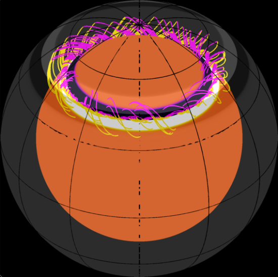
Figure 1.— Initial configuration of the magnetic flux tube introduced at $45{\arcdeg}$ and $R_{t}=5.2\times 10^{10}\,\rm cm$ and with a twist parameter q=15 (corresponding to a pitch angle of $30{\arcdeg}$). Purple indicates positive radial field and yellow indicates negative radial field.

Let’s take for simplicity $\theta=\theta_{t}=45{\arcdeg}$. Given the relations between the potentials $A$, $C$ and the three components of the magnetic field $B_{r}$, $B_{\theta}$, $B_{\phi}$, we can find an expression of the tangent of the pitch angle $\psi$ (angle between the direction of the vector magnetic field and the longitudinal direction) with respect to the initial parameters.

$$B_{r}(r,\theta_{t})=\frac{A_{0}aqR_{t}}{r^{2}}\exp\left[-\left(\frac{r-R_{t}}{a}\right)^{2}\right]$$

$$B_{\theta}(r,\theta_{t})=\frac{2A_{0}qR_{t}(r-R_{t})}{ar}\exp\left[-\left(\frac{r-R_{t}}{a}\right)^{2}\right]$$

$$B_{\phi}(r,\theta_{t})=\frac{2A_{0}R_{t}}{a}\exp\left[-\left(\frac{r-R_{t}}{a}\right)^{2}\right]$$

Hence

$$\tan\psi=\frac{\sqrt{B_{r}^{2}+B_{\theta}^{2}}}{B_{\phi}}=q\frac{\sqrt{a^{4}+4(r-R_{t})^{2}r^{2}}}{2r^{2}}$$

The pitch angle is then linked to the parameter $q$ (appearing in the expressions for the potentials $A$ and $C$) via a function of the tube radius and position. Thus, we note that the pitch angle reaches its maximum at the tube periphery (at $r=R_{t}+a$) and that it is close to $0$ at the tube center (at $r=R_{t}$). We shall note at this point that when $r=R_{t}+a$ (at the tube periphery), the term $a^{4}$ (due to the contribution of $B_{r}$) becomes very weak in comparison to the other term $4(r-R_{t})^{2}r^{2}$ (due to the contribution of $B_{\theta}$). The tangent of the maximal pitch angle is then approximately determined by the ratio $B_{\theta}/B_{\phi}$ and is in this case equal to $qa/(R_{t}+a)$.

We can now derive an expression for the winding degree of the field lines (i.e. the number of turns that the field lines make over the whole tube length $2\pi R_{t}\sin\theta_{t}$):

$$n=\frac{\pi R_{t}\sin\theta_{t}}{2a}\tan\psi$$

In all cases, except for Section 7.2, the tube radius is set to $a=10^{9}\,\,\rm cm$, about a twentieth of the depth of the modelled convection zone and is introduced at the base of the CZ at $R_{t}=5.2\times 10^{10}\,\,\rm cm$. The initial field strength $A_{0}$, the initial twist of the field lines $q$ as well as the colatitude of introduction $\theta_{t}$ will be varied in our models to investigate the influence of these various parameters.

2.3. The background hydrodynamical models

Our experiments consist in introducing the torus of magnetic field at the base of the convection zone in a spherical shell, as was presented above, in a thermally equilibrated hydrodynamical model in which the convection is or is not triggered. We then compute two different hydrodynamical models, one which is isentropic and one where we trigger the convection instability. The study of the isentropic case is the topic of Jouve & Brun Jouve [2007] and will be considered as the reference case to which the fully convective cases will be compared to.

Our numerical models are intended to be a faithful if highly simplified descriptions of the solar convection zone. Solar values are taken for the heat flux, rotation rate, mass and radius and a perfect gas is assumed since the upper boundary of the shell lies below the H and He ionisation zones. Contact is made with a real solar structure model for the radial stratification. The computational domain extends from about $0.72R_{\odot}$ to $0.96R_{\odot}$. The reference state was obtained through the 1D CESAM stellar evolution code [Morel, 1997] which uses a classical mixing-length treatment calibrated on solar models to compute convection. We are dealing with the central portion of the convection zone but neglect for this work the penetrative convection below that zone or a stable top atmosphere.

The effective viscosity and diffusivity $\nu$ and $\kappa$ are here taken to be functions of radius alone and are chosen to scale as the inverse of $\bar{\rho}^{1/3}$. We use the values: $\nu=1.13\times 10^{12}\,\rm cm^{2}.s^{-1}$ and $\kappa=4.53\times 10^{12}\,\rm cm^{2}.s^{-1}$ at mid-CZ, leading to a Prandtl number of $P_{r}=0.25$. In all cases, the spherical shell is rotating at the rate $\Omega_{0}=2.6\times 10^{-6}\,\rm rad.s^{-1}$ (corresponding to a rotation period of 28 days). In the convective cases, we trigger convection by assuming a Rayleigh number $Ra=1.85\times 10^{5}>Ra_{c}$ and setting a small and negative $dS/dr=-10^{-7}$. In these cases, we have $R_{e}=v_{conv}(r_{top}-r_{bot})/\nu_{midCZ}=120$, where the characteristic length scale is chosen to be the depth of the CZ and $v_{conv}=80\,\rm m.s^{-1}$. In the simulations, the Taylor number is $T_{a}=1.8\times 10^{6}$ and the convective Rossby number is then $R_{oc}=Ra/(T_{a}P_{r})=0.63<1$, thus ensuring a prograde differential rotation [Brun & Toomre, 2002]. The density contrast in this convective case is about 24 whereas it reaches a value of 40 in the isentropic case between the top and the bottom of the domain.

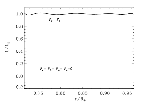
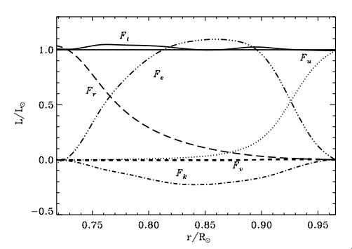
Figure 2.— Radial dependences of the main fluxes involved in the isentropic (left) and the fully convective (right) cases.

Figure 2 illustrates the contribution of various physical processes to the total energy flux through the shell, converted to luminosity and normalised to the solar luminosity, in both the isentropic and the convective model. The net luminosity, $L(r)$, and its components are defined as

$$F_{e}+F_{k}+F_{r}+F_{u}+F_{\nu}=F_{t}=\frac{L(r)}{4\pi r^{2}}$$ (11)

where

$$F_{e}=\bar{\rho}c_{p}\overline{v_{r}T},$$ (12)

$$F_{k}=\frac{1}{2}\bar{\rho}\overline{v^{2}v_{r}},$$ (13)

$$F_{r}=-\kappa_{r}\bar{\rho}c_{p}\frac{\partial\bar{T}}{\partial r},$$ (14)

$$F_{u}=-\kappa_{0}\bar{\rho}\bar{T}\frac{\partial\bar{S}}{\partial r},$$ (15)

$$F_{\nu}=-\overline{{\bf v\centerdot\cal{D}}}|_{r},$$ (16)

where $F_{e}$ is the enthalpy flux, $F_{k}$ is the kinetic energy flux, $F_{r}$ is the radiative flux, $F_{u}$ is the unresolved eddy flux, $F_{\nu}$ is the viscous flux. The thermal diffusivity $\kappa_{r}$ is derived from a 1D calibrated solar structure model [Brun et al., 2002] computed with the CESAM stellar evolution code [Morel, 1997]. We adjusted it so that the radiative flux is equal to the total flux in the whole layer in the isentropic case and is equal to the total flux at the base of the CZ for the convective case. In the latter case, the adjustment compared to the value obtained from the 1D model is small. The unresolved eddy flux $F_{u}$ is the heat flux due to SGS motions, which in our LES approach, takes the form of a thermal diffusion operating on the mean entropy gradient [Gilman & Glatzmaier, 1981, Wong & Lilly, 1994]. Its main purpose is to transport energy outward through the impenetrable upper boundary where the convective fluxes $F_{e}$ and $F_{k}$ vanish and the remaining fluxes are small.

On Fig.2, the flux balance is represented at the time the system has reached a statistical steady state. In the isentropic case, as we do not have convection, we note that the energy is exclusively transported by radiation, explaining why the total flux is equal to the radiative flux in this case.

Contrary to the isentropic case, we note that several fluxes play a role in the fully convective model. The convective flux has developed to reach an equivalent luminosity of almost 110$\%$ of the solar luminosity in the middle of the shell and the radiative and unresolved eddy fluxes carry the energy at, respectively, the bottom and the top of the domain where the enthalpy flux vanishes. The viscous flux $F_{\nu}$ is relatively small and slightly negative in most of the domain and the kinetic energy flux $F_{k}$ is, on the contrary, clearly negative in the whole convection zone. The asymmetry between the fast downflows and the broad slower upflows is responsible for the fact that the kinetic energy flux is negative. The very low value of $F_{\nu}$ confirms that the Reynolds number of these simulations is much greater than unity.

In the convective case, where different physical processes play a significant role to transport the energy, large scale flows such as differential rotation and meridional circulation (MC) are being created due to the action of convective motions. In Brun & Toomre (2002), it has been shown that convection under the influence of rotation leads to an efficient redistribution of angular momentum, energy and heat. It is found that Reynolds stresses are at the origin of the equatorial acceleration of the solar convection zone, opposed by both the meridional circulation and viscous transport, the latter being negligible in the latest solar simulations [Miesch et al., 2008]. It was also found that the latitudinal enthalpy (convective) flux is at the origin of the variation of entropy and temperature as a function of latitude, leading to warm poles and cool equatorial regions [Brun & Toomre, 2002, Brun & Rempel, 2008]. These thermal variations yield baroclinic effects that break the Taylor-Proudman constraint of invariance along the axis of rotation.

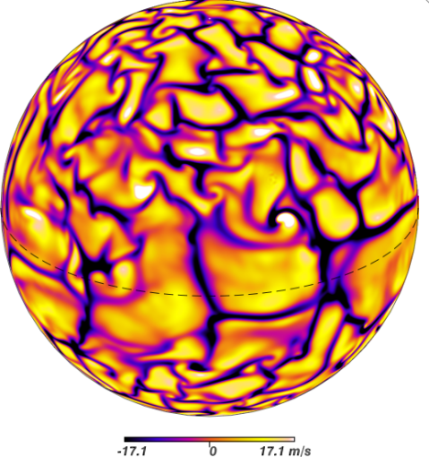
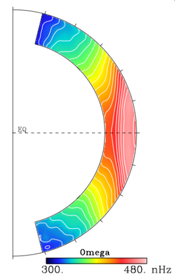
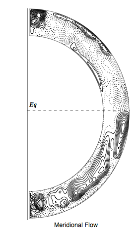
Figure 3.— Convective motions and mean flows created in the fully convective cases. The first panel shows the radial velocity profile near the top of the shell, the second shows the differential rotation profile and the right panel shows the meridional circulation, the last two panel having been averaged over longitude and time (272 days). For the meridional flow, dashed (plain) lines represent counterclokwise (clockwise) circulation and the intensity varies approximately between about -20 and 20 $\rm\,m.s^{-1}$.

Figure 3 illustrates the convective structure and the associated differential rotation and meridional flow realised in our simulations. The convective patterns are complex, time dependent and asymmetric owing to the density stratification, consisting of relatively weak, broad upflows with narrow, fast downflows around their periphery. By imposing in this model a weak entropy variation at the base of the convection zone, which mimics the presence of the tachocline, we were able to get an even more solar-like angular velocity profile [see Miesch Miesch, 2006]. The relative amplitude of this imposed variation corresponds to a pole-equator temperature difference of about 10 K. The second panel of Fig. 3 thus shows the differential rotation profile which is in good agreement with the solar internal rotation profile inferred from helioseismology [Thompson et al., 2003]. In this figure, the angular velocity of the rotating frame is 414 nHz, corresponding to a rotation period of 28 days, the angular velocity contours at mid-latitudes are nearly radial and the rotation rate decreases monotonically with increasing latitude as in the Sun. The induced meridional circulation shown on the right panel of Fig. 3 exhibits a complex profile, multicellular both in latitude and in radius. Nevertheless, close to the equator, a poleward flow of about $20\,\rm m\,s^{-1}$ strongly dominates at the surface, which is in agreement with helioseismic inversions. The fully convective model is thus far more complex that the isentropic one. Continuously the dynamics is maintained with turbulent convection, heat and angular momentum redistribution, leading to the presence of large-scale flows and asymmetric up and down flows whose various effects on a magnetic flux rope will be studied.

3. Evolution of a flux tube in an isentropic layer

In this section, we briefly summarise the results obtained in the calculations of Jouve & Brun Jouve [2007] concerning the influence of the twist of the field lines, of rigid rotation and of the initial latitude of the flux rope on its dynamical evolution in a stably stratified layer. That will ease the comparison with the convective case and complete our study with new isentropic models. Indeed, we have decided that the simulations would be more realistic if the tube radius was reduced to $10^{9}\,\rm cm$. In section 7.2, we will comment specifically on the effects of the tube radius on its evolution.

Emonet & Moreno-Insertis Emonet [1998] showed that vorticity generation in the flux tube was controlled by the competition between the gravitational torque and the magnetic tension. Consequently, by setting the gravitational torque to be equal to the projection of the Lorentz force in the equation for the azimuthal vorticity, we can determine the threshold above which the twist of the field lines can counteract the creation of two counter vortices inside the tube. We derive the following inequality for the pitch angle value:

$$\sin\psi=\frac{\sqrt{(B_{r}^{2}+B_{\theta}^{2})}}{B}\geq\sqrt{\frac{a}{H_{p}}}\times\sqrt{\left|\frac{\Delta\rho}{\bar{\rho}}\right|\frac{\beta}{2}}=\sin\psi_{min}$$ (17)

where $H_{p}$ is the pressure scale height at the base of the CZ, $\Delta\rho/\bar{\rho}$ is the density deficit inside the tube compared to the background stratification divided by the background density at the tube center and $\beta$ is the plasma-$\beta$ associated with the tube. In our case, the threshold value is equal to $0.3$ (corresponding to a pitch angle of 17.4$\arcdeg$). In most twisted cases, we use for $\sin\psi$ a value of $0.5$ (corresponding to a pitch angle of 30 $\arcdeg$), i.e. well above the threshold, so that the tube is able to rise cohesively through the entire CZ.

Rotation has also an important dynamical effect on the trajectory of the tube. Indeed, as shown in Jouve & Brun Jouve [2007] in the non-rotating case, the latitudinal component of the magnetic curvature acts to drag the tube poleward as it cannot be compensated by any equatorward force (hoop stresses). In the rotating case, a retrograde zonal flow is created inside the tube which induces a Coriolis force directed towards the Sun’s rotation axis which acts to deflect the trajectory of the tube poleward. Thus, we note that the deviation to the radial trajectory in this case is even more pronounced.

Moreover, we also showed in Jouve & Brun Jouve [2007] that the rotation has an impact on the rise time of the tube. Indeed, the radial component of the centrifugal force decreases the tube velocity so that after 6 days of evolution, the rise velocity of the tube in the non-rotating case is about 1.5 times that of the tube in the rotating case. This can be explained by the fact that the buoyancy term is modified by an extra term coming from the rotation which has the effect of limiting the efficiency of buoyancy. The flux tubes thus emerge more slowly in the rotating case.

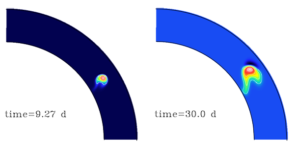
Figure 4.— Rising trajectory of a flux tube introduced with $B_{0}=10^{5}\,\rm G$. We note that the tube tends to rise parallel to the rotation axis.

We also investigated how flux tubes react when they are introduced at various latitudes. We find that the poleward drift due both to the uncompensated magnetic curvature force (hoop stresses) and the Coriolis force varies as a function of the latitude of introduction of the tube. As Moreno-Insertis et al. (1992) indicate, we can understand the poleward drift in writing the equation for the $\theta$-component of the velocity in the non-rotating case, neglecting the advection terms:

$$\centering\frac{\partial v_{\theta}}{\partial t}=-\frac{B_{\phi}^{2}}{4\pi r\bar{\rho}}\cot\theta\@add@centering$$ (18)

This equation indicates that the acceleration in the $\theta$-direction is proportional to $\cot\theta$ which is a decreasing function of $\theta$ between $0$ and $\pi/2$. As $\theta$ is here the colatitude, the acceleration at higher latitudes is thus more rapidly active than at low latitudes and as a consequence, the poleward drift is much more visible for a flux tube originally located at high latitudes.

As Choudhuri & Gilman Choudhuri [1987] first demonstrated using the thin flux tube approximation and as Fan (2008) and Jouve & Brun Jouve [2007] confirm with 3D MHD simulations, the initial strength of the magnetic field introduced at the base of the convection zone has a strong influence on the rising trajectory of the flux rope. We thus computed a new isentropic case where the initial field strength is $10^{5}\,\rm G$ and found that in this case, as illustrated on Fig. 4, the tube is strongly deviated from the radial trajectory and tends to follow a path which is parallel to the rotation axis.

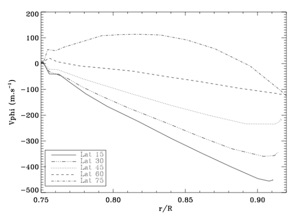
Figure 5.— Intensity of the zonal flow in the axis of the flux tube with respect to its position, for tubes introduced at various latitudes.

The deviation to the radial trajectory is due to the creation inside the tube of a retrograde zonal flow $v_{\phi}$ as soon as the magnetic structure begins its rise through the isentropic layer, as illustrated on Fig. 5. The creation of this retrograde flow is the result of the conservation of the total angular momentum $r\sin\theta\bar{\rho}(r\sin\theta\Omega_{0}+v_{\phi})$ inside the tube. Its main effect is to locally create a Coriolis force oriented toward the solar rotation axis. This Coriolis force then partially compensate the component of the buoyancy force, perpendicular to the rotation axis whereas the component parallel to the rotation axis remains the same. As soon as this compensation becomes significant, the tube is strongly influenced by the component of the buoyancy force parallel to the rotation axis and thus drifts away from the radial trajectory. We note that $v_{\phi}$ inside the tube is more and more negative to compensate for the creation of angular momentum due to the increase of $r\sin\theta$ for most cases. However, in the extremely high latitude case ($75{\arcdeg}$), $v_{\phi}$ inside the tube first increases. This is due to the fact that for this case, the curvature force is first acting to make the tube drift poleward (since the curvature force acts faster at high latitudes), so that $\sin\theta$ decreases faster than $r$ increases, leading to a decrease of $r\sin\theta\Omega_{0}$ which has to be compensated by a prograde zonal flow. For this case, $v_{\phi}$ in the tube increases until $r\sin\theta$ becomes constant and then begins to increase and only then do we recover the same behaviour as tubes introduced at lower latitudes.

Nevertheless, the initial magnetic field strength plays a role in this force balance. If the tube is weak like in the case of Fig. 4 where $B_{0}=10^{5}\,\rm G$, the Coriolis force created by angular momentum conservation is sufficiently strong to compensate the weak buoyancy force and the main component which acts on the tube will make it rise parallel to the rotation axis, which is consistent with the results of Fan (2008).

For the rise to be radial, we need to introduce sufficiently strong magnetic tubes. We found a threshold of $1.3\times 10^{5}\,\rm G$ for the initial value of the magnetic field inside the tube. For the following calculations, we thus impose an initial value above this threshold so that active regions will emerge close to the latitude where the tube was introduced.

4. Dynamical evolution of a flux tube in a fully convective shell

Table 1Key parameters of the various convective cases

Parameters	CAnt	CAtt	CAt	CBt	CCt	CAt45	CAt15	CAt60	CAt75
$B_{0}$	$5B_{eq}$	$5B_{eq}$	$5B_{eq}$	$10B_{eq}$	$2.5B_{eq}$	$5B_{eq}$	$5B_{eq}$	$5B_{eq}$	$5B_{eq}$
$\Phi_{0}/10^{23}$	$4.65$	$4.65$	$4.65$	$9.45$	$2.32$	$4.65$	$4.65$	$4.65$	$4.65$
$Latitude$	$60$	$60$	$60$	$60$	$60$	$45$	$75$	$30$	$15$
$\sin\psi$	$0$	$0.33$	$0.5$	$0.5$	$0.5$	$0.5$	$0.5$	$0.5$	$0.5$
$Re_{t}=\frac{v_{rise}a}{\nu_{midCZ}}$	$16$	$16$	$16$	$68$	$4$	$16$	$15$	$16$	$17$

Our reference isentropic case has been defined and studied. We now know that a sufficient twist of the field lines and magnetic field intensity were necessary to enable the flux tube to rise cohesively and radially through the isentropic layer. We now turn to investigate the evolution of similar tubes in a fully convective zone where mean flows are developed and maintained.

4.1. Description of the convective cases

We compute a series of models where the tube is introduced in the CZ after the convection and the mean large scale flows have self-consistently developed and we compare the results with reference cases in which we do not have convection. We thus compute an untwisted case (the initial field is exclusively oriented in the direction of the tube, i.e. $q$=0), a twisted case (with a twist above the threshold of Eq. 17), cases with tubes located at different latitudes and cases with various initial field strength. The various cases and the parameters used are summarised in Table 1.

As we said, the tube radius is set to $10^{9}\,\rm cm$, about 0.18 times the pressure scale height at the base of the CZ. The magnetic diffusivity at mid-CZ is set to the value of $1.13\times 10^{12}\rm cm^{2}\,s^{-1}$, leading to a magnetic Prandtl number of $1$, $\eta$ is made to vary as $1/\bar{\rho}^{1/3}$ like the other effective eddy diffusivities, leading to a value of $7.95\times 10^{11}\rm cm^{2}\,s^{-1}$ at the base of the CZ. The magnetic diffusivity is kept the same for all runs (except in Sect 7.2, where we investigate the influence of this parameter), we thus have the same value of the diffusive time associated to the flux tube for all cases which is $a^{2}/\eta_{baseCZ}=14.5$ days. In the convective cases, we express the initial magnetic field strength in terms of the intensity of the magnetic field which is in equipartition with the kinetic energy of the strongest downflows, this $B_{eq}$ is approximately equal to $6.1\times 10^{4}\,\rm G$. The twist of the field lines is expressed in terms of the sine of the pitch angle and can be compared to the threshold value calculated according to Eq. 17 in the isentropic case. Abbett et al. (2000) showed that this threshold may be reduced if we introduce a sufficient curvature in the magnetic structure we initially set at the base of the CZ. As we study here the evolution of initially axisymmetric flux tubes and not $\Omega$-loops, the 2D-threshold value for the twist will be used. Nevertheless, since modulation in longitude is created in certain cases by the convective motions, we may also obtain a significant curvature of the rope in our simulations and thus a lower amount of twist would likely be sufficient to maintain the tube coherence during its rise.

4.2. Interaction with convection in the standard case

In this section, we first focus on the influence of the convective motions on the tube evolution in case CAt i.e. when it is introduced at a latitude of $30{\arcdeg}$, with a fixed initial twist of about $23$ turns and an initial field strength of $3\times 10^{5}\,\,\rm G$ (i.e. $5\,B_{\rm eq}$).

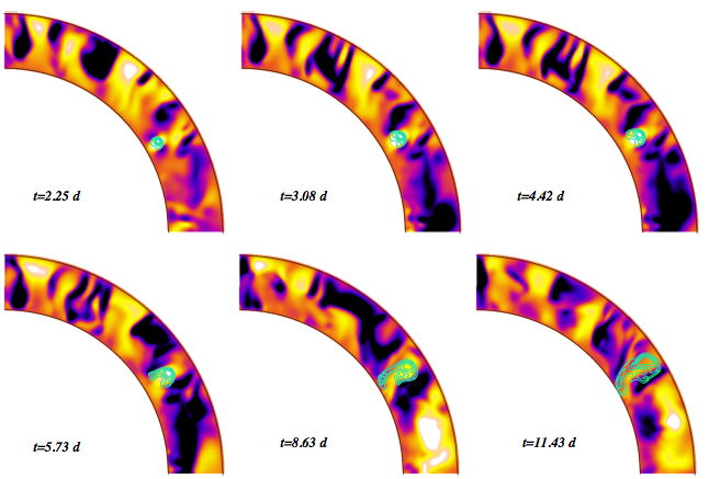
Figure 6.— Evolution of $B_{\phi}$ cut at a specific longitude and shown in a portion of the Northern hemisphere, associated with the rising tube (contours) superimposed to the evolution of the background convection represented by the coloured contours of $v_{r}$. Blue (yellow) colours represent down (up) flows, the velocities vary from -300 $\rm\,m.s^{-1}$ to 200 $\rm\,m.s^{-1}$

.

Figure 6 represents the contours of $B_{\phi}$ and of the radial velocity $v_{r}$ as the tube rises through the CZ. We first notice that the tube expands during its 12 days of evolution, to get to a radial extension of about 3 times the initial one when the tube reaches the top of domain. This expansion is due both to magnetic diffusion and to the pressure drop from the base to the top of the domain. This figure clearly shows the deformation of the shape of the tube section while it rises. The magnetic initial conditions, as we saw in Sect. 2.2, imply a perfectly circular shape of the tube section and after 12 days of evolution, the last panel of Fig. 6 shows that the tube has been squeezed at its apex and thus develops an oblate shape during its rise. Moreover, the periphery of the tube, where the magnetic field is much lower than in the apex, has thus more difficulties to make its way through the convective zone and consequently has the tendency to be dragged downwards, contrary to the rising apex. If we look closely at the convective pattern, the downward advection of the tube periphery can be easily related to the downflows appearing at each side of the tube as it rises. We then clearly see that the background convection is strongly affected by the presence of the confined magnetic field. When the magnetic structure begins its evolution, it creates its own local velocity as we can see on the first panels of Fig. 6, due to the back reaction of the Lorentz force on the velocity field. This velocity field due to the Lorentz force consists in a strong upflow in the central region (the apex) and two downflows at each side of the tube. The study of the momentum equation shows that this particular configuration of the velocity is a direct consequence of the presence of the latitudinal gradient of $B_{r}$ in the equation for $v_{r}$, which changes sign twice across the tube section. In the isentropic case, the same type of velocity field created by the presence of the magnetic tube appeared during the evolution but in this case, this configuration was much more symmetric with respect to the apex of the tube since the only background velocity was due to the tube. On the other hand, in the convective case, the velocity field created by the tube is an additional velocity to the background convection and thus a clear asymmetry is visible in the velocity field with respect to the apex. Here, especially if we focus on the 3 lower panels showing the last days of evolution, we note that the two downflows at each side of the tube are very different in extension and shape, leading to a very distorted aspect of the tube by the time it reaches the top of the domain. The effect of the Coriolis force consisting in deflecting the tube poleward is thus less visible than in the isentropic case since now the velocity field in the meridian plane also plays a very significant role in the dynamical evolution of the flux tube, as we will discuss more in section 6.

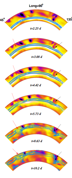
Figure 7.— Evolution of the magnetic energy cut at the latitude of $30{\arcdeg}$ (contours) superimposed to the background convection shown by a colour representation of $v_{r}$. Blue (yellow) colours represent down (up) flows, the velocities vary from -300 $\rm\,m.s^{-1}$ to 200 $\rm\,m.s^{-1}$. A black arrow indicates the location of a particular downflow a red arrow indicates the location of a particular upflow.

Since the background convection has a strong non-axisymmetric component, it is likely that the evolution of the tube will depend on the longitude, contrary to the reference isentropic case. Indeed, Fig. 7 shows the evolution of the same flux tube with the background convective motions, but projected on the $(r,\phi)$ plane. This view enables to observe the longitudinal deformation of the magnetic field due to convective up and downflows. Since our aim is to understand how active regions could be created at the solar surface, the study of the longitudinal deformation of the tube while it rises is of major interest.

The cut of the magnetic energy and $v_{r}$ is made at $30{\arcdeg}$ of latitude, where we introduce the tube initially. We thus recover on each panel of figure 7 the strong upflow we could see on the previous figure centered at the apex of the flux tube. Tracking a particular upflow (red arrow on each panel) and a particular downflow (black arrow) enables us to focus on the strong correlation existing between the regions where the magnetic structure is lifted (pinned down) and the convective upflows (downflows). Indeed, at the location of the strong downflow, the field lines are squeezed and thus retained in the solar interior, even if the tube is still globally subject to magnetic buoyancy. We thus have a competition between magnetic buoyancy and convective downflows which controls the rising behaviour of the tube, as was seen in the Cartesian study of Fan et al. (2003). In this region, even if the tube locally creates an upflow, it is not sufficient to counteract the strong background downflow and this portion of the structure is thus clearly pinned down by convection and will eventually rise significantly slower than the surrounding regions. On the contrary, the strong upflow which owes its origin both to the background convection and to the presence of the magnetic field clearly drags the field lines upward and will most probably favour flux eruption at the photosphere. We moreover see on Fig. 7 that convective plumes drift longitudinally in time due to the presence of rotation. This constitutes a major difference with previous Cartesian study where the convective structures were not influenced by rotation. The same convective plume in our simulations will thus have effects on the magnetic tube at different longitudes. A rough calculation of the drifting time of convective plumes in the middle of the convective zone at the latitude of $30\arcdeg$ shows that a convective plume could drift along $16\arcdeg$ longitudinally during this particular flux tube evolution (which lasts about 10 days). We should however take into account that the presence of the flux tube itself modifies the structure of the convective motions and thus may influence the action of convective plumes on the magnetic field, especially when it is introduced with higher intensity, as we discuss in the following section.

4.3. Interaction with convection when varying the field strength

We have just seen that a modulation in longitude appears as the tube rises through the turbulent layer, this modulation is the result of strong interactions between convective motions and the magnetic structure. These interactions are likely to be sensitive to variations of the initial magnetic intensity inside the flux tube. We thus investigate the influence of the initial magnetic field strength in these fully convective cases. Few authors [e.g. Fan et al., 2003, Murray et al., 2006] have already shown that this parameter may have a strong influence on the rising behaviour of the flux tube and on its interaction with the convective motions.

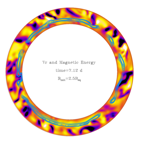
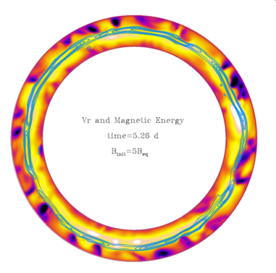
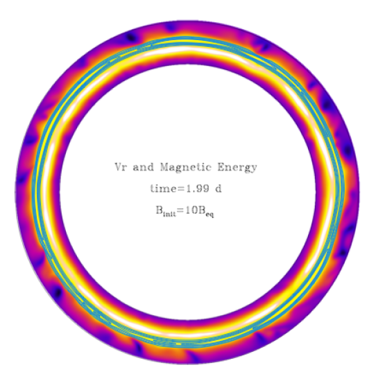
Figure 8.— Cut at $\theta=45\arcdeg$ of the radial velocity (colours) and of the magnetic energy (line contours) for 3 different initial values of the magnetic field strength (cases CCt, CAt, CBt). Yellow colours indicate upflows and blueish colours indicate downflows. The minimum velocity for all cases is about -300 $\rm\,m.s^{-1}$ and the maximal velocity (concentrated inside the tube for the strong B cases) varies, its value is about 160 $\rm\,m.s^{-1}$ for case CCt, 200 $\rm\,m.s^{-1}$ for case CAt and 420 $\rm\,m.s^{-1}$ for case CBt.

Figure 8 shows the interaction between convective motions and the rising behaviour of flux ropes introduced in the same hydrodynamical background but with three different initial values for the field strength. On the first panel, we show the result of the calculation where $B_{init}$ is approximately equal to the $2.5B_{eq}$. In this case, the correlation between the upflows (downflows) and the portions of the tube which rise more rapidly (slowly) is clearly visible. The background velocity dominates over the velocity field created by the flux rope through the Lorentz force. As a result, it is the background velocity which controls the rising behaviour of the tube. Since the initial field strength is relatively weak in this case, the convective motions first deform the tube in longitude, then the strong downdrafts pin the tube down and finally the rope loses its buoyancy by magnetic dissipation before it is able to rise through the entire convection zone. The rope is thus unable to rise to the top of the domain in this case where B is $2.5$ times the equipartition field. On the contrary, when the field is very strong compared to the equipartition field (last panel of Fig.8), the background velocity field has almost no effect on the behaviour of the rope. Its self-created velocity completely dominates the evolution and thus the tube rises almost axisymmetrically as if it was embedded in a stably stratified zone, even if a weak modulation in longitude is visible on Fig 8. In the intermediate case, where the field strength is close to 5 times the equipartition field, we note that the flux rope is strongly modulated in longitude but the whole tube emerges anyway in a relatively coherent manner. In this case, the velocity created by the tube itself is of the same order as the background velocity and the convective motions are thus able to strongly influence the tube during its dynamical evolution inside the CZ. This is an interesting behaviour since even if the tube is introduced axisymmetrically, some longitudes can be favoured and structures will be able to emerge only in few places at the solar surface, thus creating localised active regions.

As we saw, while it rises, the flux tube creates its own local velocity field which may strongly disturb the background velocity field, especially when the initial magnetic field intensity is strong compared to that of the equipartition field. This explains why the tube is more or less influenced by the convective motions as it evolves in the CZ. Indeed, if the magnetic energy of the tube is strong compared to the kinetic energy of the strongest downdrafts, the tube creates a velocity through the action of the Lorentz force which dominates against the background purely hydrodynamically-generated velocity. Since a strong upflow is thus created near the tube axis, the rising mechanism is very efficient and the tube reaches the top of the CZ in only 4 days. In the weaker cases, the velocity field created by the magnetic structure is comparable to the background velocity field and the latter is thus able to influence the behaviour of the flux rope as it rises, the rise time is in this case of about 12 days.

5. Structure of the emerging regions

We now turn to discuss the characteristics of active regions created by the buoyantly rising magnetic structures. We especially focus on the field strength, the orientation and the later evolution of the bipolar active regions. However, it has to be clarified that since our upper boundary lies at about 28 Mm below the actual solar surface, what we call “flux emergence” here is the emergence through the top of the computational domain, which is likely to be different from the emergence in the real photosphere.

5.1. Creation of bipolar regions in the standard case

Figure 9 shows a zoom, seen from above, of an emerging bipole near the top of the domain. On this figure the radial field $B_{r}$ is shown, superimposed to the background radial velocity. We can here focus on the change in the convective patterns as the flux tube emerges, on the influence of particular downflows on the magnetic structure and on the late evolution of the magnetic field after the emergence.

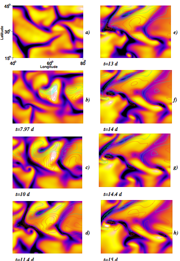
Figure 9.— Evolution of the radial field (contour lines) superimposed to the radial velocity (colour contours) at 0.96R and zoomed in a particular portion of the Northern hemisphere where a bipolar region emerges. Green (red) corresponds to positive (negative) $B_{r}$. The first panel shows the field-free region prior to the emergence and the other panels show the evolution of the magnetic structure and the velocity field from the time of emergence (2nd panel) until approximately 7 days later (last panel).

On this figure, we clearly note that the emerging phase is characterised by the appearance of the bipolar patch in a very localised portion of the ($\theta,\phi$) plane which in turn locally modifies the convective patterns. We again recover the strong upflow created by the tube and located at its apex and the downflows which appear at each side of the emerging tube. We then note that the convection organises itself very differently around the magnetic field. The strong central upflow significantly influences the background velocity field: for example, the strong downflow located on panel a) (before emergence) around the longitude of $75{\arcdeg}$ and the latitude of $30{\arcdeg}$ is modified by the appearance of magnetic structures on panel b), the downflow is squeezed and becomes less intense in the area where the tube emerges. However, this downflow is so strong at the beginning that in spite of the influence of the magnetic field, we recover its imprint during the whole evolution on all the panels. On the other hand, the upflows which were already present before the arrival at the top of the domain of the magnetic structure are enhanced by the flux emergence and for example the patch of positive radial velocity located in the middle of the first panel stays very strong during the whole evolution because it is reinforced by the emergence of the bipolar structure. The magnetic field has thus a strong influence on the modification of the convective patterns at the top of the domain but we can also focus on the influence of convection on the deformation of the rope and on its late evolution. Indeed, the strong downflows are clearly the areas where the magnetic structures have more difficulties to emerge whereas strong upflows make it very easy for the bipolar patches to appear from the beginning. On panels b) and c) in particular, we clearly see the emergence of two active regions separated by a strong downflow which causes the central area to stay deeper down in the interior. The tube thus emerges in a particular shape, with 2 distinct bipolar patches appearing and then evolving differently.

The late evolution of the flux tube after emergence also presents some interesting properties. On the first panels (b), c) and d)), the field which is brought to the surface by magnetic buoyancy dominates the evolution of the simulation since it strongly perturbs the convective motions. At this stage, we can note that the tube evolution will remain dominated by the convective motions since the diffusive time scale at the surface for regions occupying about $10\arcdeg$ in longitude is of the order of 45 days, much higher than the advection time (of the order of a few days). As the simulation evolves, the magnetic field begins to be advected horizontally by convection which tends to separate the two opposite polarities of the bipolar patches (panels e) and f)). Panels g) and h) then show the behaviour of the magnetic field and the radial velocity about 7 days after the first signs of emergence. On these panels, the field lines become stretched by the convective motions and advected towards the strong downdrafts. We then recover some features of magneto-convection when the magnetic field is less organised than one well-defined flux tube. Indeed, at this stage of evolution, the structure is much less coherent, it begins to occupy a very wide band in latitude because of the redistribution by convection.

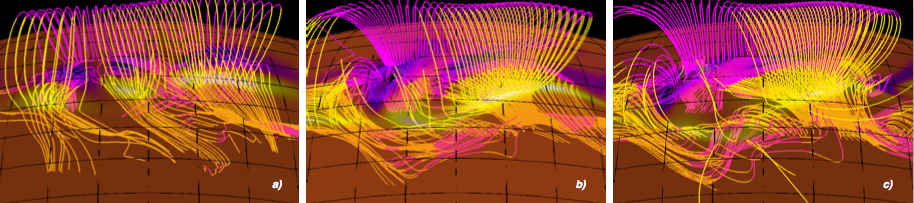
Figure 10.— Magnetic field line reconstruction below the emerging regions and above, where a potential extrapolation has been applied. Yellow (purple) lines indicate positive (negative) radial field. The three snapshots correspond to approximately panels b, e and h of Fig. 9

Figure 10 enables to see the 3D emergence of the bipolar structures, in showing the magnetic field lines reconstruction immediately below and above the top of our computational domain, at different times in the emergence process. Panel a) corresponds to the first signs of emergence, we clearly note (like panel b of Fig. 9) the North-South orientation of the bipolar patches, which becomes more and more East-West as the emergence proceeds, as is shown on panels b) and c). On these panels, the complicated structure of the flux rope starts to be visible in the interior. Indeed, we note the modulation both in latitude and in longitude of the tube when it reaches the top of the domain. Panel c) shows that the magnetic field of the tube connects with the external field during the emergence, even if some parts of the rope stay hidden in the solar interior and are not able to rise anymore. In particular, the fact that the tube axis dos not emerge and that only the upper part of the rope is visible outside the computational domain is probably responsible for the predominantly North-South orientation of the emerging patches.

This remark thus leads us to analyse in more details the evolution of the tilt angle and of other characteristics of the emerging regions, in the same spirit of the observational studies of Kosovichev & Stenflo [Koso2008, 2008].

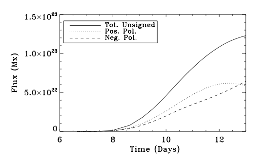
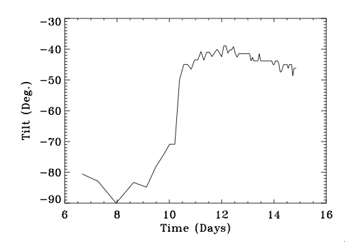
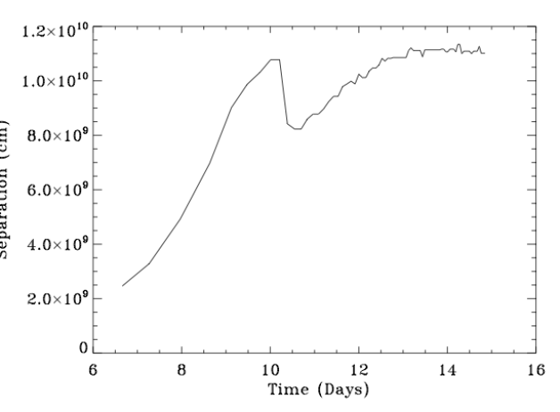
Figure 11.— Magnetic fluxes, tilt angle and footpoints separation for one of the emerging regions

Using a series of 96-min cadence magnetograms form SOHO/MDI, they analysed 715 active regions in terms of the evolution of the tilt angle, of the amount of emerging flux and of the magnetic polarities separation during emergence. We thus proceed to the same kind of analysis on our particular portion of magnetic field emerging between the longitudes of 55 and 65 degrees on panel b) of Fig. 9. We have to keep in mind that the emergence through our upper boundary (which still lies well inside the CZ) is difficult to compare directly to observed flux emergence at the photosphere. However, this type of analysis enables us to get a better insight into the processes playing a role in the evolution of magnetic flux ropes well below the photosphere, thus allowing to predict some characteristics of the structures which will actually emerge through the upper layers. The results of this analysis are shown on Fig. 11. This figure shows the evolution of the total unsigned flux (together with the contribution of the positive and negative polarities), the tilt angle and the magnetic polarities separation. The amount of flux first sharply increases during the first 3 or 4 days after the first signs of emergence and then reaches a saturation and starts to decrease as the opposite magnetic polarities stop separating. After about 4 days after emergence, the separation between the two opposite polarities is not modified by emergence anymore and the concentrations of radial field start to be advected by convection and by magnetic diffusion on a longer time scale than the rise time of our flux rope, leading to a saturation of the footpoints separation visible on the last panel of Fig. 11. Finally, we investigate the evolution of the tilt angle of our emerging bipolar region and note that the orientation is mainly North-South on the first days of emergence (the tilt angle is then equal to about $-90\arcdeg$). Bipolar regions are thought to be the imprints of the flux tube axis emerging, creating a positive radial field at one foot of the emerging loop and a negative radial field at the other foot. In these simulations, we do not clearly see the axis of the tube emerging, the radial field which is observed is the one existing at the apex of the tube because it is twisted. However, as the emergence proceeds, we see that the orientation of the bipolar structure changes because of the convective motions, the 2 polarities are advected more and more independently and the orientation becomes more East-West (a tilt angle of $-40{\arcdeg}$ is reached when the active region begins its decay) both because the structure is made sufficiently arched by the radial velocity and because the horizontal velocity acts differently on the 2 regions of opposite polarity. By applying the same kind of analysis for particular active regions created by tubes initially located at the latitudes of $45\arcdeg$ (case CAt45) and $15\arcdeg$ (case CAt15), we can assess how the tilt angle changes as a function of the initial latitude. We do not see a clear difference in the tilt angle for case CAt45 in comparison to case CAt described above, mainly because their rise time, the amount of flux emerging and the arching of the magnetic structure are similar. We thus not clearly see different effects of the physical processes involved to modify the tilt angle (Coriolis force, advection by convection, twist of the field lines) between these 2 cases. On the other hand, in case CAt15, where the tube is introduced at the latitude of $15\arcdeg$, the tilt angle reaches a smaller value (about $-20\arcdeg$ when the active region starts to decay). This can be explained mainly by the difference in the rise time of this particular tube compared to the others, as we will discuss in detail in Sect. 6.1. Since the rise time for this tube is longer, the Coriolis force may have the time to significantly affect the tube orientation when it reaches the surface. Moreover as we will see in Sect. 7.2, magnetic diffusion plays the role of untwisting the flux ropes. Since the rise time is longer in this case, diffusion has acted more on this tube and the tube appears less twisted when it emerges, which leads to a tilt angle reduced in comparison to the cases at higher latitude. This particular feature may be in agreement with Joy’s law which states that bipolar structures emerging at lower latitudes have a smaller tilt angle than regions emerging at higher latitudes at the beginning of a new solar cycle.

5.2. Influence of the field strength on emergence

The initial magnetic field strength has a strong influence on the way the structure will emerge as it reaches the top of the computational domain, thus creating active regions with various morphological and dynamical characteristics.

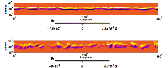
Figure 12.— Cut at $r=0.93R$ of $B_{r}$ for case CBt (lower panel) and case CAt (upper panel). We clearly note the difference between the two computations in the way the magnetic flux emerges.

Figure 12 shows the radial magnetic field close to the top of the shell by the time the axis of the flux rope is situated approximately at $0.93R$, for cases CAt and CBt. When the tube is strong, the tube emerges at all longitudes with very small azimuthal modulation even if the strong downflows have been able in some portions of the tube to keep it from emerging as fast as in the upflow regions. We also notice that the flux rope emerges at approximately the latitude of introduction, no poleward slip is thus visible in this case. On the contrary, in the weak B case, some longitudes are clearly favoured and some ’active regions’ can be identified. We indicated on Fig. 12 the intensity of the emerging $B_{r}$, which is about a few kiloGauss in case CAt. On the other hand, when the tube is introduced with a flux of about $10^{24}\,\rm Mx$, as in the strong B case, the emerging radial field is of the order of a few tens of kiloGauss. In this case, a strong flux loss would then have to be experienced by the tube during its rise up to the photosphere to match the observations of sunspots magnetic field at the solar surface.

We also note that in the weak B case, the latitude of emergence is slightly higher than the latitude of introduction of the flux tube at certain longitudes. Indeed, we see on the bottom panel of Fig.12 that the emerging structures appear at latitudes higher than the latitude of introduction ($30{\arcdeg}$). This drift could be explained partly by the poleward slip instability and the action of the Coriolis force which were already observed in the isentropic case but may also be due to the action of the mean meridional flow as we now discuss in section 6.

6. Influence of mean flows

As stated in sect. 2.3, convection in a spherical shell establishes and continuously maintains mean flows. We wish to take benefit of our self-consistent simulations to address the question of how meridional flows and differential rotation may influence the tube-like structure during its rise through the CZ.

6.1. Differential rotation

The results coming from the study of flux tubes in a stably stratified spherical layer in Jouve & Brun Jouve [2007] showed that the dynamical evolution of flux tubes could be modified if they were introduced at various latitudes. Indeed, for instance, we saw that the poleward drift was more rapidly active for tubes introduced at high latitudes, thus leading to a strong deviation of these tubes to their radial trajectory. In the fully convective cases, we saw that the convective patterns as well as the profile of the large-scale flows strongly varied in latitude and longitude (see Fig.3). It is thus likely that the differences between tubes introduced at various latitudes will be even more pronounced in these cases.

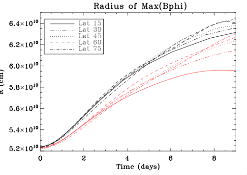
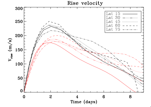
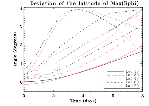
Figure 13.— Comparison of the evolution of flux tubes introduced at different latitudes (cases CAt15, CAt, CAt45, CAt60, CAt75) in red with their isentropic counterparts in black. The first panel shows the position in radius of the maximum of $B_{\phi}$ versus time, the second panel is the velocity of the tube versus time and the last panel shows the difference between the position in latitude of the max of $B_{\phi}$ and the latitude of introduction.

Figure 13 shows the temporal evolution of weak tubes initially located at the latitude of $15\arcdeg$, $30\arcdeg$, $45\arcdeg$, $60\arcdeg$ and $75\arcdeg$. The first panel shows the position in radius of the maximum of $B_{\phi}$ (corresponding to the location of the tube axis) as the tube rises through the CZ, the second panel indicates the rise velocity of each tube and finally the third panel represents the deviation in latitude of the position of $\rm max(B_{\phi})$ compared to the latitude of introduction. We confirm that tubes introduced at various latitudes have different evolutions. Looking at panels 1 and 2, we see that the tube initially located close to the equator (at $15\arcdeg$) can be clearly distinguished from the others, especially in the convective case. This tube indeed reaches its maximal velocity before the others and the decelerating phase is so significant that it almost stops rising after it has reached the middle of the convection zone. After 8 days of evolution, its rise velocity indeed becomes very weak (about $10\rm\,m.s^{-1}$) and the radial position of the tube axis reaches its maximum at about $5.95\times 10^{10}\,\rm cm$ in the CZ. On the other hand, the three tubes initially located in the upper part of the Northern hemisphere keep on rising until the tube periphery reaches the top boundary condition where the radial velocity vanishes. This difference between tubes introduced at various latitudes is less significant in the isentropic case. For example, after 9 days of evolution in an isentropic layer, the distance travelled by a tube introduced at $15{\arcdeg}$ is $5\%$ less than that of a tube introduced at $45{\arcdeg}$. In the convective case, this difference reaches $20\%$. This may be explained by the presence of a differential rotation in the convective case. We showed in the isentropic case that the buoyancy term appearing in the evolution of the radial velocity was proportional to $g-r\sin^{2}\theta\Omega^{2}$ with $\theta$ the colatitude and $\Omega$ the rotation rate. We showed that at constant $\Omega$, an increase in the colatitude $\theta$ caused a decrease of this term and thus of the efficiency of buoyancy, resulting in a slower emergence at higher colatitude or lower latitude. In this convective case here, a solar-like differential rotation is present in the bulk of the CZ. The profile of this differential rotation is conical between $25\arcdeg$ and $60\arcdeg$ and cylindrical under $25\arcdeg$. This differential rotation may explain the major reduction of velocity in the cases at low latitudes in comparison to the cases at high latitudes as the strong rotation at low latitudes is very likely to decrease the rise velocity of the tube to such a point that it is not able to rise through the upper part of the CZ. However, the effect of the centrifugal force which modifies the buoyancy may be weak compared to the total gravitational acceleration and thus the slowdown of tubes introduced in a convective background could also be caused by the Coriolis force due to the retrograde flow created along the tube.

Panel 2 shows that because of the convective downdrafts acting to pin the flux tube down, the rising velocity is reduced compared to the isentropic case. Indeed, when the tube was introduced at $45\arcdeg$, it reached a maximal velocity of about $230\,\rm m.s^{-1}$ while the maximal velocity is only $180\,\rm m.s^{-1}$ in the convective case, i.e. $21\%$ less. For a tube introduced at the latitude of $15{\arcdeg}$, the difference is even more pronounced and reaches the value of $27\%$, which in turn leads the tube embedded in the convective background to be stopped by the time it reaches the middle of the CZ. The effects of intense downflows again appear to be very significant in these weak B cases and we thus show the dramatic changes that the introduction of a convective environment implies on the simulations of rising flux tube. It has to be noticed that the ratio between the rise velocity of a section of the tube located in an upflow and another located in a downflow is about 1.5. Thus for example in case CAt45 where the average rise velocity is about $180\,\rm m.s^{-1}$, the region of the tube located in a particular upflow can reach a velocity of $210\,\rm m.s^{-1}$ whereas a part located in a downflow will hardly reach $140\,\rm m.s^{-1}$. We note that these values are still lower than the rise velocity reached by a tube introduced in a stable isentropic layer, possibly showing the influence of the strong downflows over the whole tube which tries to keep its coherent structure during its rise. Our study clearly shows the effects of a non-uniform rotation on magnetic ropes, especially the severe constraints on low-latitudes emergence it introduces. Although the emergence through our upper boundary may have little resemblance with emergence at the real solar surface, this particular finding may still be interesting to consider when analysing the properties of the solar cycle which shows a strong decrease in the number of sunspots appearing at low latitudes in the declining phase. Only sufficiently strong flux tubes would be able to rise at low latitudes, which is confirmed by some observations of sunspot magnetic field during a cycle. Indeed, sunspots emerging at higher latitudes seem to possess brighter umbrae, thus indicating weaker magnetic fields [Norton & Gilman, 2004], although this tendency seems to be slight and thus possibly due to an observational bias [Livingston et al., 2006] and has not been confirmed by other space-based studies [Mathew et al., 2007]. If we suppose that such effects happening deep inside the convection zone are visible during emergence at the surface, a possible explanation would thus be that differential rotation makes it more difficult for weak tubes to emerge at low latitudes and not only that they are drifting away from the radial trajectory as they rise, as they conclude in Norton & Gilman (2004).

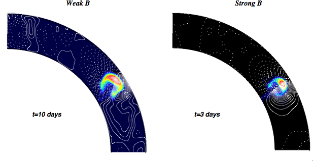
Figure 14.— Cut of $B_{\phi}$ at a particular longitude in the Northern hemisphere for cases CAt (left panel) and CBt (right panel) superimposed to the background meridional flow. For the meridional flow, dashed (plain) lines represent counterclockwise (clockwise) circulation. We note the strong meridional circulation created by the tube itself when B is initially strong.

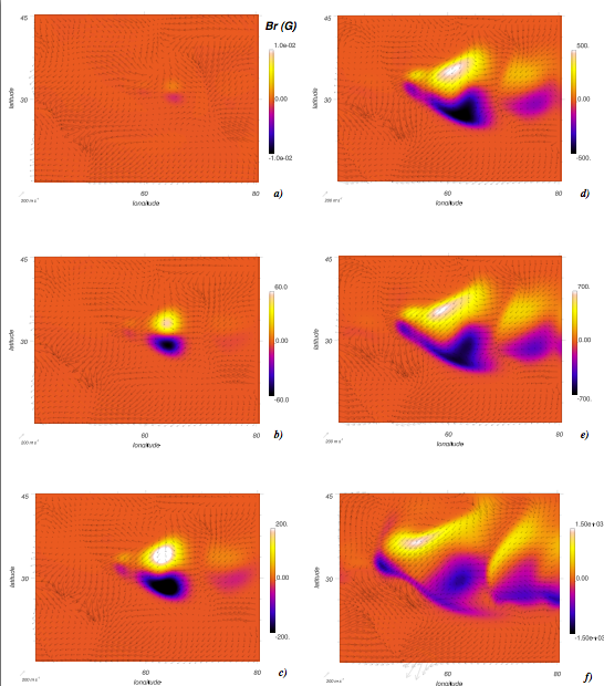
Figure 15.— Influence of the emerging magnetic flux on the surface flow structure. We superimpose the radial field (coloured contours) and the surface velocity field (arrows) on a particular portion of the longitude-latitude plane in case CAt.

Panel 3 confirms the results in the isentropic case that showed that the poleward drift of the flux tubes due both to the uncompensated magnetic curvature force and to the Coriolis force acting on the tube is more active at high latitudes. Indeed, it is clear that at $60\arcdeg$ and $75\arcdeg$, as soon as the tube has started rising, it is strongly deviated from the radial trajectory. We recover the particular behaviour of the tube introduced at $75\arcdeg$ which undergoes an equatorward drift because of the prograde flow being created in its interior. However, this deviation to the radial trajectory is less pronounced than in the isentropic cases, where for instance after 6 days of evolution, a tube initially located at $60\arcdeg$ had deviated by $3.8\arcdeg$. In the same case here, the deviation angle hardly reaches $2.8\arcdeg$ at the same time, i.e. $26\%$ less. This difference is mainly due to the longitudinal flow appearing in the tube interior as soon as the tube begins to rise, which is much stronger in the isentropic cases than in the convective ones. This can be understood by considering the non-axisymmetric deformation of the tube in the convective case. This leads to friction between the magnetic structure and its surroundings which in turn transfers angular momentum to the mass elements in the tube and therefore leads to less retrograde motion. For instance, after 4 days of evolution, the tube embedded in the isentropic layer has created a longitudinal flow of about $-30\,\rm m.s^{-1}$ whereas the tube embedded in the convective zone has not developed any significant zonal motion, it is still rotating at the same velocity as its surroundings because the non-uniform rotation in radius plays a role in the conservation of the flux rope angular momentum. As a consequence, the intensity of magnetic field needed for tubes to rise radially may be overestimated in the isentropic case. W now move to the study of the influence of the meridional flow, which may also act to advect the magnetic structure away from the radial trajectory.

6.2. Meridional circulation

As we said in the first section, meridional flows are maintained by buoyancy forces, Reynolds stresses, pressure gradients, Maxwell stresses and Coriolis forces acting on the differential rotation. Since these relatively large forces nearly cancel one another, this circulation can be thought of as a small departure from (magneto)geostrophic balance, and the presence of a localised magnetic field can clearly influence its subtle maintenance.

Indeed, for two different initial magnetic intensity in the flux rope, it is interesting to focus on the streamfunction of the background meridional flow. Figure 14 shows the position of the flux rope close to the end of its evolution through the CZ, superimposed to the streamfunction of the meridional velocity. We clearly see that the situation is different in the two cases. In the strong B case, the contours of the MC streamfunction are concentrated around the flux rope and are very symmetric with respect to the tube apex. In this case, this observed velocity field is created by the flux rope itself through the back-reaction of the Lorentz force on the flow and it is completely dominant compared to the background velocity. This velocity field structure, characterised by a strong upflow at the tube apex and two downdrafts at each side of the tube drives the tube radially upward, without any latitudinal drift since the magnetic structure is not sensitive to the background MC. The situation is clearly different in the weak B case. In this case, the velocity field created by the tube itself is of the same order as the background meridional flow and thus the rope is very likely to be advected in a particular direction whether it is embedded in a poleward or in an equatorward flow. Here we note that by the time it reaches the top of the domain, the tube is drifting northward partly because of the poleward drift phenomenon we mentioned in the isentropic case. Thus the tube ends up in a poleward flow at this particular longitude, which reinforces the poleward advection of the magnetic structure.

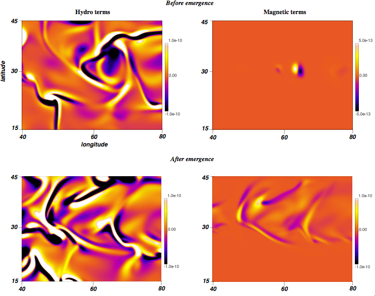
Figure 16.— Hydrodynamical and magnetic terms playing a role in the evolution equation of the radial vorticity, just before emergence and after emergence.

Several observational studies with MDI/SOHO data [Haber et al., 2003, 2004, Hindman et al., 2004, Gizon, 2004, Gizon et al., 2001, Švanda et al., 2008] showed that emergence of new magnetic flux could generate perturbations on the observed surface horizontal flow. Consequently, we can focus our study on the modification of this horizontal flow by the emergence of our flux tube modulated by convection. Fig. 15 shows the superimposition of the emerging radial magnetic field and the horizontal velocity field close to the upper limit of the domain ($0.96R_{\odot}$) for case CAt during the emergence process, and until the intensity of the emerging radial field has reached a value of about $1500\,\rm G$. On the first panel, the magnetic flux has hardly emerged (the intensity of the radial field is below $10^{-2}\,\rm G$ and the horizontal velocity field thus presents a pattern which is almost not modified by the magnetic tube. We then get the emergence of the magnetic structure, which is showed by the growing intensity of the radial field. As the structure emerges, the changes in the horizontal velocity field due to the magnetic forces are slight but visible. Indeed, the intensity of the flow is growing because of the presence of magnetic field, which is especially clear on panels e) and f) around the positive polarity which is dominant for this particular bipolar patch. Moreover, regions of converging flows become more confined between the actives longitudes, as we can see for example on panels d), e) and f) where the converging flow (associated with a strong downflow lane around $70{\arcdeg}$) are particularly concentrated between the different emerging bipolar structures. Another striking point is the acceleration of the retrograde zonal flow during emergence, as a result of the azimuthal velocity created within the tube because of angular momentum conservation.

Consequently, slight modifications can be seen on the structure of the horizontal flow as the magnetic structures emerge. To be more quantitative, we focus on the creation of radial vorticity due both to hydrodynamical terms and to magnetic terms just before and after emergence and how the magnetic field plays a role in this balance to locally modify the flow structure. Indeed, following the evolution of the radial vorticity enables to track the evolution of the horizontal flow profile since the radial vorticity can be expressed as follows:

$$\omega_{r}=\frac{1}{r\sin\theta}\left[\frac{\partial(\sin\theta v_{\phi})}{\partial\theta}-\frac{\partial v_{\theta}}{\partial\phi}\right]$$ (19)

The evolution equation for $w_{r}$ can be decomposed on 4 hydrodynamical terms (not depending on $B$ or any of its derivatives) and 3 magnetic terms, as follows:

$$\frac{\partial\omega_{r}}{\partial t} = \underbrace{\left[({\bf\omega_{a}}\cdot{\bf\nabla}){\bf v}-({\bf v}\cdot{\bf\nabla}){\bf\omega_{a}}-({\bf\nabla}\cdot{\bf v}){\bf\omega_{a}}-{\bf\nabla}\times(\frac{1}{\bar{\rho}}{\bf\nabla}\cdot{\bf\cal D})\right]_{r}}_{\mbox{hydro terms}}$$ (20)

$$+ \underbrace{\left[\frac{1}{\bar{\rho}c}\left(({\bf B}\cdot{\bf\nabla}){\bf j}-({\bf j}\cdot{\bf\nabla}){\bf B}-{\bf j}\cdot{\bf\nabla}(\frac{1}{\bar{\rho}})\right)\right]_{r}}_{\mbox{magnetic terms}}$$

with ${\bf\omega_{a}}$ the absolute vorticity defined by the relation ${\bf\omega_{a}}={\bf\nabla\times v}+2{\bf\Omega_{0}}$.

Figure 16 shows the value of the sum of only the hydrodynamical terms and of only the magnetic terms in the radial vorticity evolution equation 20, just before emergence (corresponding to panel a) of Fig. 15) and significantly after (corresponding to panel f) of Fig. 15). We note that at the very beginning of emergence, when a small bipolar patch begins to emerge with the North-South orientation, the magnetic terms are more than 2 orders of magnitude smaller than the hydro terms. The latter completely determine the behaviour of the horizontal flow, especially the advection term (second in the RHS of Eq. 20), which is dominant and peaks at about $10^{-9}\,\rm s^{-2}$, whereas the dominant magnetic term hardly reaches $10^{-11}\,\rm s^{-2}$. On the other hand, when the structure has sufficiently emerged (the structure and strength of the radial field at this time are showed on the last panel of Fig. 15), the magnetic terms start to play a role in the vorticity generation and thus on the horizontal flow structure. They have increased by about 2 orders of magnitude and since the norm of the hydrodynamical terms stays close to the same values, all those terms begin to equally compete. We note that the magnetic source terms for radial vorticity concentrate everywhere the magnetic field gradients are sharp. This can be seen especially around the strong positive polarity around 55 degrees of longitude and 40 degrees of latitude. In this region, the structure has emerged and thus a strong gradient in longitude of all components of the the field will act to produce currents which will in turn play a role in the radial vorticity generation. We thus conclude that the horizontal flow is modified by magnetic fields preferentially where strong gradients of field exist, for instance at the edge of the emerging structure, in agreement with what was concluded from the analysis of Fig. 15.

7. Dynamical evolution in a fully convective shell: influence of the parameters

We now turn to investigate how the significant parameters of the reference case influence the flux tube in its rise through the convection zone in the case where we have a fully turbulent convection developed in the bulk of the computational domain. We will also look for new key parameters which may constrain the behaviour of the magnetic rope during its dynamical evolution.

7.1. Role of twist

We saw that the twist of the field lines plays a fundamental role in the ability of the flux tube to rise cohesively in a stratified layer. Moreover, observations of active regions show that a certain amount of twist of the field lines is often detected [Schmieder et al., 1996], especially in regions called sigmoids. These sigmoids take the shape of a reversed S in the Northern hemisphere and of a S in the Southern hemisphere, sign of the hemispheric law for helicity (which is directly related to the twist) which is found to be preferentially negative in the North and positive in the South. These regions are of particular interest because they are known to be favoured places for the triggering of CMEs or other violent events at the solar surface. Recent numerical simulations [Török & Kliem, 2005, Fan & Gibson, 2004, Amari et al., 2000] show that a twisted flux rope is always present at a certain point in the flux emergence (prior to the emergence for Török & Kliem and built during the emergence for Amari et al.) and that the twist is sometimes the determining factor for the eruption to occur (via the kink-instability for example).

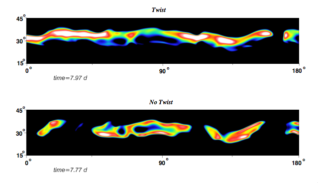
Figure 17.— Cut of $B_{\phi}$ at a specific radius after approximately 10 days of evolution in case CAt (upper panel) and in case CAnt (lower panel). We clearly note the splitting of the flux tube in the untwisted case.

Consequently, both simulations and observations show the fundamental role of the twist of the field lines while flux emerges and a further investigation of this parameter is then particularly important. Figure 17 shows the behaviour of a flux tube embedded in a fully convective shell in an untwisted case (lower panel) and a twisted case (upper panel). We recover the fact that a sufficient twist of the field lines is needed for the tube to maintain its integrity while it rises through the CZ. Indeed, we note that in the untwisted case, the tube splits into two parts while it rises because of the uncompensated vorticity generation created inside the flux rope by the gravitational torque, as was discussed in Sect. 3 and in Jouve & Brun Jouve [2007] in the reference case. On the contrary, the right panel of Fig. 17 illustrates the fact that the twisted magnetic structure has kept its tube-like shape by the time it has almost reached the top of the shell.

We also note that the deformation of the rope due to the convective up and down flows is more pronounced in the untwisted case. Indeed, since the tube splits into two separate concentrations of flux, the two resulting structures are magnetically less strong and are thus more sensitive to the surrounding convective motions. Moreover, when the tube is twisted, magnetic tension acts to prevent convective downdrafts from penetrating into the magnetic structure. The tube is thus more cohesive and thus less distorted than in the untwisted case (even if the modulation in longitude is already very significant) and is able to reach the top of the computational domain and emerge.

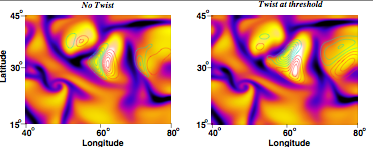
Figure 18.— Zoom, seen from above at $r=0.93R_{\odot}$ of an emerging region in case CAnt (left panel) and a twisted case where the twist is just above the threshold (right panel). These snapshots correspond to approximately the same time of evolution as panel 3 of Fig. 9, we clearly note the difference in the orientation of the main bipolar region.

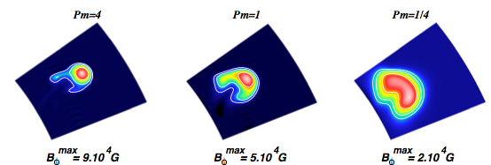
Figure 19.— Longitudinal magnetic field after 5 days of evolution with $Pm=4$, 1 and 1/4.

Figure 18 shows that the twist of the field lines is of major interest for the orientation of the emerging bipolar structures as we already saw in the preceding section. In the non-twisted case, when the tube is sufficiently strong to reach the top of the CZ, the emerging radial field creates bipolar regions which have the right East-West orientation. However, these active regions have a very significant extension in latitude because of the two counter vortex rolls which drift apart horizontally and this is not what is observed in the Sun where active regions are very localised in latitude. If the twist of the field lines just reaches the threshold, we see that the orientation of the patches becomes East-West quite early in the emerging process. Indeed in this case, we observe the radial field coming from the two feet of the arched (because of convective down and up flows which deform the tube) portion of the tube sooner than in the very twisted case where the radial field due to the twist dominates. As a consequence, if we follow the evolution of the tilt angle for this case as we did for case CAt on Fig. 11, we see that it becomes East-West much more rapidly after emergence and above all that the final tilt angle we get is about $-15\arcdeg$, i.e. closer to the observations at this particular latitude. Moreover, this case has an initial number of turns of 14 (corresponding to a pitch angle of about $20\arcdeg$) and thus if we consider that the emerging region occupies about $20\arcdeg$ in longitude when it has expanded at the surface, the number of turns in this particular bipolar region would be of about 0.78, in agreement with the typical value observed in most active regions. This case thus seems to be able to reproduce several interesting features of active regions such as their orientation (even if the tilt angle is still high in comparison to observations but could be reduced with more arched structures), their amount of twist and the field strength inside the regions of opposite polarities, which is of the order of 1 kiloGauss, as in case CAt.

7.2. Influence of the diffusivities

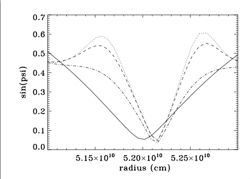
Figure 20.— Measure of the sine of the pitch angle (1st panel), of the longitudinal field (2nd panel) and of the transverse field (3rd panel) at the initial time (plain line) and after only 5 hours of evolution for tubes with $Pm=4$ (dotted line), $Pm=1$ (dashed line) and $Pm=1/4$ (dash-dotted line).

In this section, we investigate the effects of varying the magnetic diffusivities in our models of flux tubes evolution, keeping all the other parameters constant. We vary $\eta$ from a value of $1.13\times 10^{12}\rm cm^{2}\,s^{-1}$ in the middle of the convection zone (corresponding to a magnetic Prandtl number of unity) to a value of $2.83\times 10^{11}\rm cm^{2}\,s^{-1}$ (leading to $Pm=4$) and to a value of $4.54\times 10^{12}\rm cm^{2}\,s^{-1}$ (leading to $Pm=1/4$). It has been shown in previous thin flux-tube studies [Moreno-Insertis et al., 1995] that a strong entropy gradient could be built between the tube interior and its surroundings during its rise through the CZ. As a consequence of higher entropy within the tube, the external gas pressure decreases faster than the internal pressure and may finally reach the same value, forcing the magnetic pressure to approach zero. The tube apex then experiences a so-called explosion which causes this part of the tube to stop rising and leads to an amplification of the magnetic field in the non-exploded parts [see Rempel & Schüssler, 2001, for a full MHD treatment of this process]. In our simulations where the high diffusion of entropy may wash out the gradients responsible for such effects, our tubes do not undergo any explosion and stay magnetically buoyant from the base of the CZ to the top of our computational domain. However, for this section, we wanted to keep the same convective background and at the same time keep the value of $Pr=0.25$ unchanged since it has proved to be favorable to a solar-like differential rotation (Brun & Toomre 2002; Miesch et al. 2006). This has dictated our choice of $\nu$ and $\kappa$ and thus we did not consider those parameters as free anymore. At the present time, the ASH code uses effective eddy diffusivities to represent momentum, heat and magnetic field transport by motions which are not resolved by the simulation. They are allowed to vary in radius but are independent of latitude, longitude and time. This type of treatment for the unresolved motions thus affects all spatial scales and it has to be stated that this may have a significant influence on the evolution of spatially localised structures such as the magnetic flux tubes introduced in our simulations and the strong subsequent currents created. Nevertheless, we note that the diffusion term as a whole preferentially acts where the magnetic field gradients (or equivalently the currents) are the strongest. An improved treatment of sub-grid-scale motions in ASH is currently being considered, which would take into account a spatial dependence of the transport coefficients. The influence of this new treatment on our results will have to be checked but for this work, we focus on the major differences which can already be pointed out between cases at various $Pm$, thus showing the particular care with which diffusion has to be considered in this type of simulations.

After 5 days in the convection zone, the tubes introduced with various magnetic diffusivities have evolved in a very different way, as shown on Fig. 19. We clearly see the difference in the expansion of the magnetic field concentration as the tube rises, each cut in the (r,$\theta$) having the same dimensions. Since the diffusive time goes from $a^{2}/\eta=$ 58 days for $Pm=4$ to 14.5 days when $Pm=1$ to 3.6 days when $Pm=1/4$ (using the value of the magnetic diffusivity at the base of the convection zone), it is straightforward to note that the intensity of the magnetic field retained in the flux rope after the same time of evolution in the convection zone is strongly decreased (by a factor 4.5 between $Pm=4$ and $Pm=1/4$) when the magnetic diffusivity is increased. Moreover, we see that the two sharper and fainter structures at each side of the tube visible on the first panel are completely lost because of the action of diffusion in the two other cases. Finally, the major consequence of increasing the magnetic diffusivity can be seen on the last panel of the figure, in the $Pm=1/4$ case. Not only has the tube significantly expanded compared to the others but it seems to have split apart because of an insufficient amount of twist to maintain its coherence. We investigate the evolution of the twist of the field lines in the 3 different cases to understand how a high magnetic diffusivity has caused the tube to lose its coherence during its rise.

Figure 20 shows the profile of the sine of the pitch angle and of the longitudinal and transverse magnetic field at the location of the flux tube at the starting time and after 5 hours of evolution for the various cases. We note that the magnetic structures in the $Pm=1$ and $Pm=4$ cases stiffen in comparison to the initial configuration, a feature which is mainly due to the creation of current sheets ahead of the flux tube when it begins its rise through the CZ.

The main results that we deduce from this analysis is that the transverse field gets a sharper structure than the longitudinal field as soon as the tube begins its rise. This property leads to a faster diffusion of transverse field than of longitudinal field. Indeed, panel 2 shows that in the $Pm=1/4$ case, the maximum of $B_{\phi}$ is $69\%$ of the maximum for the $Pm=4$ case whereas the maximum of the transverse field only reaches $42\%$ of the maximal transverse field for the less diffusive case. As a consequence, the pitch angle is strongly reduced by this faster diffusion of transverse fields, the tension force is not sufficient anymore to counteract the vorticity generation inside the tube and thus the pitch angle quickly goes under the threshold value needed to maintain the tube coherence.

7.3. Influence of the tube radius

We now turn to investigate the influence of the tube radius, which is closely linked to the study of variations of the magnetic diffusivity which we addressed in the preceding section. Indeed, since the diffusive time is proportional to the square of the tube radius, magnetic diffusion will act faster on smaller tubes and we must thus take into account its potential effects on our tubes. Consequently, we choose to compute models with $Pm=4$, which will limit the effects of diffusion, and we modify the tube radius from $10^{9}\,\rm cm$ to $2\times 10^{9}\,\rm cm$ and to $5\times 10^{8}\,\rm cm$. The initial magnetic field is chosen to be equal to $5B_{eq}$ and the sine of the pitch angle equal to 0.5, as in our standard case CAt. To compute these models, a very high resolution is needed, in particular, in the smallest tube case ($5\times 10^{8}\,\rm cm$), we use 1024 points in latitude, 2048 in longitude and 450 in radius, leading to a number of points to describe the tube section of 26 points in radius and 10 points in latitude. In the $10^{9}\,\rm cm$ case with $Pm=4$, we also increase the resolution in latitude compared to our previous cases (1024 points instead of 512, although the results are qualitatively similar) but keep 256 points in radius, we thus end up with $N_{r}=32\times N_{\theta}=20$ points to resolve the tube section. Finally, for the $2\times 10^{9}\,\rm cm$ tube, the number of points in the tube is also $N_{r}=32\times N_{\theta}=20$ (as the total resolution in latitude is now 512). In all cases, the number of points is thus significant enough to have a good description of the magnetic field profile inside the rope.

Figure 21.— Cut of $B_{\phi}$ in the Northern hemisphere at a specific longitude for tubes with an initial radius of $5\times 10^{8}\,\rm cm$ (top panel), $10^{9}\,\rm cm$ (mid-panel) and $2\times 10^{9}\,\rm cm$ (bottom panel) after about 6.6 days of evolution in a convective model with $Pm=4$.

Figure 21 shows the result of the study of the influence of the tube radius on its evolution in the convection zone. We focus on the structure of the longitudinal field $B_{\phi}$ at two different longitudes and at a specific time, close to the end of the evolution (after 6.6 days). Not surprisingly, the concentration of magnetic flux in the tube interior is broader when the tube is larger and the amount of flux retained in the tube is smaller in the $5\times 10^{8}\,\rm cm$-radius tube since the magnetic diffusion has started to play a significant role, even if choosing $Pm$ to be equal to 4 made the diffusive time to be about 14 days in the smallest tube case. As a consequence, we note on the first panel that the convection has acted to modulate the tube in longitude since the left structure has evolved very differently from the right one. This asymmetry is also visible on the second panel (where the tube radius was originally $10^{9}\,\rm cm$) but is less clear on the largest tube calculation, for which the competition with convective motions is in favour of the magnetic structure. The main differences in the evolution of these tubes with various radii reside in the wake that they create during their rise. We can focus on these differences by zooming on the section of the tube at a particular longitude, as shown on Fig. 21. In the smallest tube cases, we clearly see two sharp structures being created at both sides of the magnetic rope and one central tail (especially visible on the 2 last panels) which enables to approximately follow the trajectory of the tube axis as it rose through the CZ. These structures and their properties were studied in great detail in Emonet & Moreno-Insertis (1998) and their analysis apply to what we obtain in our simulations. We can add to this study that a modification of the tube extension in radius leads to a different evolution of the wake and thus of the vorticity distribution inside the tube. Indeed, the wake extends further behind the tube apex when the tube is smaller, the 2 sidelobes where the vorticity is concentrated are located significantly behind the apex whereas in the bigger radius case, the 2 sidelobes appear to stay very close to the main flux concentration, as was seen in previous calculations in Cartesian geometry.

8. Conclusion

One of the main goals of this work was to investigate what type of emerging structures we obtain in the upper part of the convection zone when we introduce an axisymmetric flux tube at its base. We saw that all the various flows existing in the convection zone could strongly influence the behaviour of the tube while it rises. If the tube is sufficiently weak to be sensitive to the presence of mean flows and turbulent convection close to the surface, we saw that an azimuthal modulation was created by convective motions. This modulation in longitude on the magnetic structure produces arched regions, the center of which will emerge before the “sides” (or the “feet”). As a consequence, in the first phases of emergence, only a portion of the tube is visible at the surface and emerges as a bipolar region. The orientation of such a bipolar structure will first be North-South but as the emergence proceeds, different processes will act to produce the tilt angle corresponding to the statistical Joy’s law. As was pointed out before, both the Coriolis force acting differently on the two legs of the loop and the twist of the field lines are able to produce an angle compared to the East-West direction before and during emergence [e.g. Fan, 2008]. We here showed an example of a flux tube possessing an amount of twist just above the threshold. This simulation can reproduce several characteristics of active regions, namely the amount of twist in the bipolar structure, the magnetic field strength in each polarity and the orientation of the two polarities. We moreover emphasise that convective motions advecting separately the two opposite polarities of the patch of magnetic field can also be a source of the tilting of active regions, which could not have been investigated in previous Cartesian or non-convective studies. To disentangle between those various physical processes acting to produce the tilt angle necessary for some kind of dynamos to work such as Babcock-Leighton dynamos [see Dikpati & Charbonneau, 1999], we now need to concentrate on an individual active region emerging at the solar surface and its particular morphological and dynamical properties. To do so, we plan to investigate the rise of non-uniformly buoyant flux tubes from the solar interior to the surface in a fully convective environment possessing mean flows, as in the present work.

Indeed, we showed in this study the particular effect of differential rotation on tubes introduced at different latitudes. As rotation has the property to slow tubes down during their rise and that rotation is stronger at lower latitudes, it would imply that tubes emerging at lower latitudes would have to be more intense to make their way up to the surface. The mean meridional flow proves to have smaller effects on the flux tube rise but may well modify the trajectory of structures slightly in superequipartition with the strongest downflows at the base of the convection zone. Moreover, our simulations show that the magnetic terms can play a significant role in the horizontal flow maintenance close to the surface and thus that the appearance of magnetic patches at the top of our domain locally modifies the surface flow structure. Mean flows should thus be taken into account in future simulations of rising magnetic structures, since their interactions with flux ropes are far from being negligible.

We now need to consider the introduction of such flux tubes in a magnetised environment where different scales would interact and the dynamo field would probably modify the results of the present study. In particular, reconnection in the interior of our computational domain between our well-defined flux tube and a more turbulent chaotic small-scale field is likely to modify the amount of twist of the field lines contained in the rope. Indeed, how twist is created in the solar interior and how it is modified during the rise of magnetic structures are still questions to be addressed. Several observational studies of helicity in active regions [Schmieder et al., 1996] tend to show that a systematic twist of the field lines can be observed but the intensity of which would be small compared to what is needed in simulations for tubes to rise coherently from the base of the CZ to the surface. We thus need to reconcile the theoretical and observational approaches in studying the evolution of the twist of the field lines of a flux tube embedded in a realistic magnetised convection zone. We plan to do so in a future work. Moreover, to allow some direct comparison to observations, the implementation of a stable layer in the ASH code in which a full MHD treatment of the emergence will be applied is currently worked on. The results of this more realistic upper boundary and the emergence at the top of this new domain will be the topic of a following paper.

References

- Abbett et al. [2000] Abbett, W. P., Fisher, G. H., & Fan, Y. 2000, ApJ, 540, 548
- Amari et al. [2000] Amari, T., Luciani, J. F., Mikic, Z., & Linker, J. 2000, ApJ, 529, L49
- Archontis et al. [2005] Archontis, V., Moreno-Insertis, F., Galsgaard, K., & Hood, A. W. 2005, ApJ, 635, 1299
- Browning et al. [2006] Browning, M. K., 0Miesch, M. S., Brun, A. S., & Toomre, J. 2006, ApJ, 648, L157
- Brun & Toomre [2002] Brun, A.S., & Toomre, J. 2002, ApJ, 570, 865
- Brun et al. [2002] Brun, A. S., Antia, H. M., Chitre, S. M., & Zahn, J.-P. 2002, A&A, 391, 725
- Brun et al. [2004] Brun, A.S., Miesch, S.M. & Toomre, J. : 2004, ApJ, 614, 1073
- Brun & Rempel [2008] Brun, A. S., & Rempel, M. 2008, Space Science Reviews, 173
- Brummell et al. [2002] Brummell, N., Cline, K., & Cattaneo, F. 2002, MNRAS, 329, L73
- Caligari et al. [1995] Caligari, P., Moreno-Insertis, F. & Schüssler, M. : 1995, ApJ, 441, 886
- Cattaneo et al. [2006] Cattaneo, F., Brummell, N. H. & Cline, K. S. : 2006, MNRAS, 365, 727
- [12] Chae, J., & Moon, Y.-J. 2005, ApJ, 629, 1110
- Cheung et al. [2007] Cheung, M. C. M., Schüssler, M., & Moreno-Insertis, F. 2007, A&A, 467, 703
- [14] Choudhuri, A. & Gilman, P. : 1987, ApJ, 316, 788
- Cline [2003] Cline, K. S. 2003, Ph.D. Thesis
- Clune et al. [1999] Clune, T. L., Elliott, J. R., Glatzmaier, G. A., Miesch, M. S., & Toomre, J. 1999, Parallel Comput., 25, 361
- D’Silva & Choudhuri [1993] D’Silva, S., & Choudhuri, A. R. 1993, A&A, 272, 621
- Dikpati & Charbonneau [1999] Dikpati, M., & Charbonneau, P. 1999, ApJ, 518, 508
- Dorch et al. [2001] Dorch, S. B. F., Gudiksen, B. V., Abbett, W. P., & Nordlund, Å. 2001, A&A, 380, 734
- [20] Emonet, T. & Moreno-Insertis, F. : 1998, ApJ, 492, 804
- Fan et al. [1994] Fan, Y., Fisher, G. H., & McClymont, A. N. 1994, ApJ, 436, 907
- Fan [2004] Fan, Y. 2004, Living Rev. Solar Phys.
- Fan et al. [2003] Fan, Y., Abbett, W.P. & Fisher, G. H. 2003, ApJ, 582, 1206
- Fan & Gibson [2004] Fan, Y., & Gibson, S. E. 2004, ApJ, 609, 1123
- Fan [2008] Fan, Y. 2008, ApJ, 676, 680
- Gilman & Glatzmaier [1981] Gilman, P. A., & Glatzmaier, G. A. 1981, ApJS, 45, 335
- Gizon [2004] Gizon, L. 2004, Sol. Phys., 224, 217
- Gizon et al. [2001] Gizon, L., Duvall, T. L., Jr., & Larsen, R. M. 2001, Recent Insights into the Physics of the Sun and Heliosphere: Highlights from SOHO and Other Space Missions, 203, 189
- Hindman et al. [2004] Hindman, B. W., Gizon, L., Duvall, T. L., Jr., Haber, D. A., & Toomre, J. 2004, ApJ, 613, 1253
- Haber et al. [2004] Haber, D. A., Hindman, B. W., Toomre, J., & Thompson, M. J. 2004, Sol. Phys., 220, 371
- Haber et al. [2003] Haber, D. A., Hindman, B. W., & Toomre, J. 2003, GONG+ 2002. Local and Global Helioseismology: the Present and Future, 517, 103
- [32] Jouve, L., & Brun, A.S. 2007, Astronomical Notes, 328, 1104
- [33] Kosovichev, A. G., & Stenflo, J. O. 2008, ApJ, 688, L115
- Kosugi et al. [2007] Kosugi, T., et al. 2007, Sol. Phys., 243, 3
- Livingston et al. [2006] Livingston, W., Harvey, J. W., Malanushenko, O. V., & Webster, L. 2006, Sol. Phys., 239, 41
- [36] Longcope, D. W., Fisher, G. H., & Arendt, S. 1996, ApJ, 464, 999
- Magara [2004] Magara, T. 2004, ApJ, 605, 480
- Martinez et al. [2008] Martínez-Sykora, J., Hansteen, V., & Carlsson, M. 2008, ApJ, 679, 871
- Mathew et al. [2007] Mathew, S. K., Martínez Pillet, V., Solanki, S. K., & Krivova, N. A. 2007, A&A, 465, 291
- Miesch et al. [2000] Miesch, M. S., Elliott, J. R., Toomre, J., Clune, T. L., Glatzmaier, G. A., & Gilman, P. A. 2000, ApJ, 532, 593
- [41] Miesch M. S., Brun A. S. & Toomre J. 2006, ApJ, 641, 618
- Miesch et al. [2008] Miesch, M. S., Brun, A. S., DeRosa, M. L., & Toomre, J. 2008, ApJ, 673, 557
- Moffatt [1978] Moffatt, H. K. 1978, Cambridge, England, Cambridge University Press, 1978. 353 p.,
- Morel [1997] Morel, P. 1997, A&AS, 124, 597
- Moreno-Insertis et al. [1992] Moreno-Insertis, F., Schüssler, M. & Ferriz Mas, A. : 1992, A&A, 264, 686
- Moreno-Insertis et al. [1995] Moreno-Insertis, F., Caligari, P., & Schuessler, M. 1995, ApJ, 452, 894
- Murray et al. [2006] Murray, M. J., Hood, A. W., Moreno-Insertis, F., Galsgaard, K. & Archontis, V., 2006, A&A, 460, 909
- Norton & Gilman [2004] Norton, A. A., & Gilman, P. A. 2004, ApJ, 603, 348
- Parker [1993] Parker, E. N. 1993, ApJ, 408, 707
- Rempel & Schüssler [2001] Rempel, M., & Schüssler, M. 2001, ApJ, 552, L171
- Scharmer et al. [2002] Scharmer, G. B., Gudiksen, B. V., Kiselman, D., Löfdahl, M. G., & Rouppe van der Voort, L. H. M. 2002, Nature, 420, 151
- Schmieder et al. [1996] Schmieder, B., Demoulin, P., Aulanier, G., & Golub, L. 1996, ApJ, 467, 881
- [53] Schüssler, M. 1979, A&A, 71, 79
- Silvers et al. [2009] Silvers, L. J., Vasil, G. M., Brummell, N. H., & Proctor, M. R. E. 2009, arXiv:0901.2388
- Spruit [1981] Spruit, H.C. : 1981, A&A, 98, 155
- Spruit & van Ballegooijen [1982] Spruit, H.C., & van Ballegooijen, A.A. : 1982, A&A, 106, 58
- Švanda et al. [2008] Švanda, M., Kosovichev, A. G., & Zhao, J. 2008, ApJ, 680, L161
- Thomas et al. [2002] Thomas, J. H., Weiss, N. O., Tobias, S. M., & Brummell, N. H. 2002, Nature, 420, 390
- Thompson et al. [2003] Thompson, M. J., Christensen-Dalsgaard, J., Miesch, M. S., & Toomre, J. 2003, ARA&A, 41, 599
- Török & Kliem [2005] Török, T., & Kliem, B. 2005, ApJ, 630, L97
- van Driel-Gesztelyi [2002] van Driel-Gesztelyi, L. 2002, SOLMAG 2002. Proceedings of the Magnetic Coupling of the Solar Atmosphere Euroconference, 505, 113
- Wissink et al. [2000] Wissink, J. G., Matthews, P. C., Hughes, D. W., & Proctor, M. R. E. 2000, ApJ, 536, 982
- Wong & Lilly [1994] Wong, V. C., & Lilly, D. K. 1994, Physics of Fluids, 6, 1016