Diffusive Corrections to $P_{N}$ Approximations

Abstract

In this paper, we investigate moment methods from a general point of view using an operator notation. This theoretical approach lets us explore the moment closure problem in more detail. This gives rise to a new idea, proposed in [14, 15], of how to improve the well-known $P_{N}$ approximations. We systematically develop a diffusive correction to the $P_{N}$ equations from the operator formulation — the so-called $D_{N}$ approximation. We validate the new approach with numerical examples in one and two dimensions.

1 Introduction

Developing simplified methods for the simulation of radiative transfer requires taking into account the physical situation that will be analyzed. There are two important limits: optically thick and optically thin media. In optically thin media there are very few particles that interact with the radiation. The distances that photons would typically travel before they are scattered or absorbed are therefore very long compared to the domain size. On the other hand, in optically thick regimes those distances are very short compared to the domain size.

[Optically thin medium.] [Optically thick medium.]

Figure 1: Path of a photon in optically thin and optically thick media.

The different regimes can be characterized by the mean free paths $\chi$ for scattering and $\varepsilon$ for absorption. Large mean free paths represent an optically thin regime, small mean free paths represent optically thick regimes. One problem in this characterization is, that many materials are optically thick in a specific frequency range and optically thin in other ranges. Additionally, there is a transition regime between the two. This is the region of mean free paths between optically thin and thick media. In this regime, photons travel further than in optically thick situations, but not far enough as that the regime counts as optically thin.

An example of an optically thin regime is radiation propagating in vacuum. Optically thick regimes can be found in glass cooling processes or combustion chambers. There are also situations where all these regimes play a role. For instance, during the reentry of a space craft into the atmosphere the regime goes from optically thin (space) through a transition (higher atmosphere) into optically thick (lower atmosphere).

Due to large mean free paths in optically thin regimes it is possible to track the trace of many single photons until they leave the computational domain or undergo absorption. This is the basic idea of ray tracing and Monte Carlo methods. If there are very few scattering events, following the path of one photon is rather simple. These particle methods are often used in astrophysics where the physical conditions are usually in a way that these methods can be applied successfully. For examples see [18, 23, 29, 30].

In optically thick regimes, following the path of a single photon is almost impossible because it undergoes too many scattering events before it reaches its destination (leaving the computational domain or being absorbed). Therefore, other methods are used. They are usually based on the diffusion approximation [20], e.g. the Simplified $P_{N}$ approximation [10, 11, 19, 27] or flux-limited diffusion [12].

The transition regime is the region of optical depth that is located between optically thin and optically thick regimes. Methods that work well in optically thin media are computationally too expensive in these regimes. Methods that work well in optically thick media, on the other hand, give poor results for low order approximations and have high computational costs if one increases the order. Therefore, in these regimes new methods have to be developed.

These new approximations have to recover traditional reduced models for small mean free paths. Further, in the transition regime, they have to be more accurate than the simplified models and should be solvable more efficiently than the full kinetic approaches.

The field of use for transition regime models can be found in stand-alone solvers for problems that lie completely within the optically thick and transition regime. For problems where the order of the mean free path also covers the optically thin regime, the new approaches could be used in hybrid methods.

In this work, our starting point will be moment methods. These are usually derived based on the assumption that in highly scattering materials the photon distribution is driven toward a local equilibrium Therefore, the radiative intensity distribution is almost isotropic at every point. If this is the case, instead of treating the full intensity distribution, we can restrict our analysis to quantities that are averages of the directional distribution function over all directions. These quantities are e.g. the spectral energy distribution, the spectral flux and the spectral pressure. Averages of products of intensity distribution with directional test functions are called moments of the intensity function. Often, one is only interested in these averaged quantities.

There is a variety of moment closures. One of the first was the $P_{N}$ closure, which was developed by Chandrasekhar [4]. Other approaches include the minimum entropy closure [1, 7, 17, 12, 13]. A recent approach applies methods from the study of dynamical systems to moment closure [9, 22].

In Section 2 we introduce the main concept of moment methods in an operator notation. This theoretical approach lets us explore the moment closure problem in more detail. This investigation gives rise to a new approach, proposed in [14, 15], of how to improve the well-known $P_{N}$ approximations (Section 3). Using the operator formulation, we systematically develop a diffusive correction to the $P_{N}$ equations — the so-called $D_{N}$ approximation. We do not treat boundaries here; they are considered in [8]. The partial differential equations behind the operator notation are developed for a simple example in Section 4, before we develop the general $P_{N}$ and $D_{N}$ equations in Sections 5 and 6 respectively. Numerical examples in one and two dimensions are then shown in Section 7. We find that the solution of the $D_{N}$ equations is at least as accurate as the solution of the $P_{N}$ equation of two orders higher.

2 Moment Models and Deviation Decomposition

We consider radiation in a spatial domain $X$ with boundary $\partial X$ whose intensity $I(t,x,\Omega)$ at time $t\geq 0$, position $x\in X$, and direction $\Omega\in S^{2}$ is governed by the frequency-averaged radiative transfer equation (RTE)

$$\frac{1}{c}\partial_{t}I(t,x,\Omega)+\Omega\cdot\nabla_{x}I(t,x,\Omega)+(\sigma(x)+\kappa(x))I(t,x,\Omega)\\ =\frac{\sigma(x)}{4\pi}\int_{S^{2}}\Phi(x,\Omega\cdot\Omega^{\prime})I(t,x,\Omega^{\prime})\,d\Omega^{\prime}+\kappa(x)B(T(x))+Q(t,x,\Omega)\,.$$ (2.1)

Here $\sigma(x)$ and $\kappa(x)$ are the scattering and absorption coefficients, $\Phi(x,\Omega\cdot\Omega^{\prime})>0$ is the scattering redistribution function, $B(T(x))>0$ is the blackbody emission intensity at temperature $T(x)>0$, and $Q(t,x,\Omega)$ is the emission due to other sources. The scattering redistribution function satisfies the normalization

$$\int_{S^{2}}\Phi(x,\Omega\cdot\Omega^{\prime})\,d\Omega=1\,.$$ (2.2)

The fact that $\sigma(x)$, $\kappa(x)$, and $B(T(x))$ are independent of $\Omega$, while $\Phi(x,\Omega\cdot\Omega^{\prime})$ depends on $\Omega\cdot\Omega^{\prime}$ is consistent with a stationary, isotropic background medium. The fact that these functions are independent of $t$ means that the heat capacity of this medium is large.

We will express the different parts of equation (2.1) in terms of operators.

Definition 2.1.

We define the operators

$$({\mathcal{A}}I)(t,x,\Omega) =\Omega\cdot\nabla_{x}I(t,x,\Omega)\,,$$ (2.3a)

$$({\mathcal{S}}I)(t,x,\Omega) =\frac{\sigma(x)}{4\pi}\int_{S^{2}}\Phi(x,\Omega\cdot\Omega^{\prime})\,I(t,x,\Omega^{\prime})\,d\Omega^{\prime}\,,$$ (2.3b)

$$({\mathcal{K}}I)(t,x,\Omega) =(\kappa(x)+\sigma(x))I(t,x,\Omega)-({\mathcal{S}}I)(t,x,\Omega)\,,$$ (2.3c)

$$({\mathcal{L}}I)(t,x,\Omega) =({\mathcal{A}}+{\mathcal{K}})I(t,x,\Omega)\,,$$ (2.3d)

$${\mathcal{Q}}(t,x,\Omega) =\kappa(x)B(T)+Q(t,x,\Omega)\,.$$ (2.3e)

Here ${\mathcal{A}}$ is advection, ${\mathcal{S}}$ is scattering, ${\mathcal{K}}$ is total interaction due to scattering and absorption, and ${\mathcal{Q}}(t,x,\Omega)$ is total emission. Using these operators the RTE reads

$$\frac{1}{c}\partial_{t}I(t,x,\Omega)+{\mathcal{L}}I(t,x,\Omega)={\mathcal{Q}}(t,x,\Omega)\,.$$ (2.4)

We impose homogeneous boundary conditions. Let

$$\Gamma=\partial X\times S^{2}\,,\quad\text{and}\quad\Gamma^{\pm}=\{(x,\Omega)\in\Gamma\;:\;\pm n(x)\cdot\Omega>0\}\,,$$ (2.5)

where $n$ is the outward unit normal vector. Appropriate boundary conditions are

$$I(t,x,\Omega)=0\qquad\forall t>0\;\text{and}\;(x,\Omega)\in\Gamma^{-}\;.$$ (2.6)

Together with the initial condition

$$I(0,x,\Omega)=I_{0}(x,\Omega)\,,$$ (2.7)

we have a well-posed problem. Under certain (physically reasonable) assumptions on the scattering and absorption coefficients $\sigma$ and $\kappa$, and for ${\mathcal{Q}}\in L^{2}(]0,t_{1}[\times X\times{S^{2}},\mathbb{R})$, ${\mathcal{Q}}(t,x,\Omega)\geq 0$ there exists a unique solution $I\in\{I\in\mathbb{D}_{t}\;:\;I=0\;\text{on}\;\Gamma^{-}\}$ (cf. [5]), where

$$\mathbb{D}_{t}\subset L^{2}(]0,t_{1}[\times X\times{S^{2}},\mathbb{R}).$$ (2.8)

Moment methods have a long history [4, 6]. Nevertheless they are still used for solving radiative or neutron transfer problems in situations where computational time is of concern. The main idea of moment methods is to derive an approximation to the radiative intensity distribution with respect to its directional moments. This relation is used to find an expression for the closure relation. There are several ways to find such approximations. The $P_{N}$ approach expresses the radiative intensity distribution as a series expansion of spherical harmonics. The minimum entropy approaches use an expression with an exponential function. But, independent of how these methods approximate the intensity, all of them have in common that the unknown coefficients in their expansion are somehow related to the directional moments of the intensity function.

Moments are directional averages of the intensity distribution multiplied with a test function that depends on the direction $\Omega$. As test functions one can choose between several possibilities. We will use spherical harmonics, denoted by $Y^{k}_{l}$, cf. Appendix A. There are several reasons for choosing these functions. First, they form an orthonormal basis of the function space $\mathbb{H}^{m}({S^{2}},\mathbb{C})$ and therefore, after transformation also of $L^{2}(S^{2},\mathbb{R})$. Hence, they can be used for a complete description of the dependence of the intensity distribution on the direction $\Omega$. In other words, each intensity distribution can be represented by the series expansion

$$I(t,x,\Omega)=\sum_{l=0}^{\infty}\sum_{k=-l}^{l}{\mathbf{I}}^{k}_{l}(t,x)Y^{k}_{l}(\Omega)\;,$$ (2.9)

with moments

$${\mathbf{I}}^{k}_{l}(t,x)=\int_{{S^{2}}}\overline{Y^{k}_{l}(\Omega)}I(t,x,\Omega)d\Omega\;.$$ (2.10)

To deal with spherical harmonics and the related moments we define

Definition 2.2.

Moments of the radiative intensity are generated by the operator

$$\begin{split}\textswab{m}^{k}_{l}\;:\;&\mathbb{D}_{t}\to L^{2}(]0,t_{1}[\times X,\mathbb{C})\\ &I(t,x,\Omega)\mapsto\int_{{S^{2}}}\overline{Y^{k}_{l}(\Omega)}I(t,x,\Omega)d\Omega\;,\end{split}$$ (2.11)

and we write for the moment of order $l$ and degree $k$

$${\mathbf{I}}^{k}_{l}(t,x)=\textswab{m}^{k}_{l}\left(I(t,x,\Omega)\right)\;.$$ (2.12)

We allow the moments to be complex valued. A real-valued approximation to the radiative intensity is obtained by taking the real part of these equations. The moments depend on time and space. For convenience we neglect this in the notation if it is clear to what we are referring and write ${\mathbf{I}}^{k}_{l}={\mathbf{I}}^{k}_{l}(t,x)$.

A vector ${\mathbf{I}}$ of all moments belongs to

$$\mathbb{M}_{t}=\left\{{\mathbf{I}}=(\ldots,{\mathbf{I}}^{k}_{l},\ldots)^{T}\;:\;l\in\mathbb{N}_{0},\;k\in\{-l,\ldots,l\}\right\}\subseteq l^{2}\left(L^{2}(]0,t_{1}[\times X,\mathbb{C})\right),$$ (2.13)

where $l^{2}$ denotes the space of all square summable sequences. We introduce

Definition 2.3.

We define the “Intensity to Moment” operator

$$\begin{split}{\mathcal{M}}\;:\;&\mathbb{D}_{t}\to\mathbb{M}_{t}\\ &I(t,x,\Omega)\mapsto{\mathbf{I}}(t,x)\;.\end{split}$$ (2.14)

The inverse transformation is given by the “Moment to Intensity” or “Expansion” operator

$$\begin{split}{\mathcal{E}}\;:\;&\mathbb{M}_{t}\to\mathbb{D}_{t}\\ &{\mathbf{I}}(t,x)\mapsto\sum_{l=0}^{\infty}\sum_{k=-l}^{l}{\mathbf{I}}^{k}_{l}(t,x)Y^{k}_{l}(\Omega)\;.\end{split}$$ (2.15)

By their construction the operators ${\mathcal{M}}$ and ${\mathcal{E}}$ are linear, bounded and continuous. Furthermore, it is easy to see that both operators are bijective.

So far we have replaced the unknown dependence in $\Omega$ by infinitely many unknown moments. This does not help us to solve the RTE. A usual approach to overcome this problem is to assume that finitely many moments are sufficient to describe the intensity function. This reduces the amount of unknowns to a finite number and the problem can be handled much more easily. Assuming that only the moments up to order $N$ are relevant gives an approximation $I_{N}(t,x,\Omega)$ to $I(t,x,\Omega)$

$$I(t,x,\Omega)\approx I_{N}(t,x,\Omega)=\sum_{l=0}^{N}\sum_{k=-l}^{l}{\mathbf{I}}^{k}_{l}(t,x)Y^{k}_{l}(\Omega)\;.$$ (2.16)

and it holds

$$\lim_{N\to\infty}I_{N}(t,x,\Omega)=I(t,x,\Omega).$$ (2.17)

The finite set of moments can be represented by the vector

$${\mathbf{I}}_{N}=({\mathbf{I}}^{0}_{0},{\mathbf{I}}^{-1}_{0},{\mathbf{I}}^{0}_{1},\ldots,{\mathbf{I}}^{N-1}_{N},{\mathbf{I}}^{N}_{N})^{T}$$ (2.18)

and we define the set of restricted vectors of moments as

$$\mathbb{M}_{t}^{N}=\left\{{\mathbf{I}}_{N}\in\left(L^{2}(]0,t_{1}[\times X,\mathbb{C})\right)^{(N+1)^{2}}\right\}\;.$$ (2.19)

Note that $\mathbb{M}_{t}^{N}$ is isomorphic to a subspace of $\mathbb{M}_{t}$.

We restrict ourself to approximations of the radiative intensity of odd orders. There are several reasons for this. First of all, even order approximations do not contain more information than odd order approaches. Therefore, they only introduce more moments and are computationally more expensive without giving any advantage. A second point for choosing just odd order approaches is given in [6, Chapter 10, § 3.2]. There it is shown, that boundary conditions for even order approximations are much less accurate than for odd order models.

Analogous to Definition 2.3, we define

Definition 2.4.

The “restricted Intensity to Moment” operator is

$$\begin{split}{\mathcal{M}}_{N}\;:\;&\mathbb{D}_{t}\to\mathbb{M}_{t}^{N}\\ &I(t,x,\Omega)\mapsto{\mathbf{I}}_{N}(t,x)\;.\end{split}$$ (2.20)

The inverse transformation is given by the “restricted Moment to Intensity” operator

$$\begin{split}{\mathcal{E}}_{N}\;:\;&\mathbb{M}_{t}^{N}\to\mathbb{D}_{t}^{N}\subset\mathbb{D}_{t}\\ &{\mathbf{I}}_{N}(t,x)\mapsto\sum_{l=0}^{N}\sum_{k=-l}^{l}{\mathbf{I}}^{k}_{l}(t,x)Y^{k}_{l}(\Omega)=I_{N}(t,x,\Omega)\;.\end{split}$$ (2.21)

with

$$\mathbb{D}_{t}^{N}=\left\{I_{N}\in\mathbb{D}_{t}\;:\;I_{N}(t,x,\Omega)=\sum_{l=0}^{N}\sum_{k=-l}^{l}{\mathbf{I}}^{k}_{l}(t,x)Y^{k}_{l}(\Omega)\right\}\;.$$ (2.22)

The only difference between the operators ${\mathcal{E}}$ and ${\mathcal{E}}_{N}$ is the restriction on the domain and the range. The restriction of $\operatorname{Range}({\mathcal{E}}_{N})$ on $\mathbb{D}_{t}^{N}$ ensures that the injectivity is inherited from ${\mathcal{E}}$. Therefore, ${\mathcal{E}}_{N}$ is still bijective. $\mathbb{D}_{t}^{N}$ is the subspace of $\mathbb{D}_{t}$ that contains only those intensity functions, which can be represented by moments up to order $N$. Due to the bijectivity of ${\mathcal{E}}_{N}$, working with either the set of moments up to order $N$ or the approximated intensity distribution $I_{N}(t,x,\Omega)$ is equivalent.

Lemma 2.5.

The combined operator

$$\begin{split}{\mathcal{P}}_{N}\;:\;&\mathbb{D}_{t}\to\mathbb{D}_{t}\\ &I(t,x,\Omega)\mapsto{\mathcal{E}}_{N}{\mathcal{M}}_{N}I(t,x,\Omega)\end{split}$$ (2.23)

is a projection.

Proof.

We have to show that ${\mathcal{P}}_{N}^{2}I(\Omega)={\mathcal{P}}_{N}I(\Omega)=I_{N}(\Omega)$ holds. Writing down the intensity function as series expansion, applying the operators as defined in Definition 2.4 and additionally using the orthonormality property of the spherical harmonics gives the result. ∎

By using ${\mathcal{P}}_{N}$, we can define the projection onto the orthogonal complement $\widetilde{\mathbb{D}}_{t}^{N}\perp\mathbb{D}_{t}^{N}$ (with $\mathbb{D}_{t}=\mathbb{D}_{t}^{N}\oplus\widetilde{\mathbb{D}}_{t}^{N}$) by $\tilde{\mathcal{P}}_{N}=\operatorname{Id}-{\mathcal{P}}_{N}$. This gives rise to

Definition 2.6.

The radiative intensity can be decomposed into a component that can be described by finitely many moments $I_{N}(\Omega)$ and a deviation

$$\tilde{I}_{N}(\Omega)=\tilde{\mathcal{P}}_{N}I(\Omega)\;.$$ (2.24)

This splitting is called deviation decomposition.

We call $\tilde{I}_{N}(\Omega)$ the deviation because it is the difference between the full radiative intensity $I(\Omega)$ and the component $I_{N}(\Omega)$ that can be represented by finitely many moments:

$$\begin{split}I(\Omega)&={\mathcal{P}}_{N}I(\Omega)+(\operatorname{Id}-{\mathcal{P}}_{N})I(\Omega)\\ &=I_{N}(\Omega)+\tilde{\mathcal{P}}_{N}I(\Omega)\\ &=I_{N}(\Omega)+\tilde{I}_{N}(\Omega)\;.\end{split}$$ (2.25)

Lemma 2.7.

The RTE can be decomposed into an equivalent coupled system of finitely many moment equations and one deviation equation

$$\frac{1}{c}\partial_{t}{\mathbf{I}}_{N}+{\mathcal{M}}_{N}{\mathcal{L}}{\mathcal{E}}_{N}{\mathbf{I}}_{N}+{\mathcal{M}}_{N}{\mathcal{L}}\tilde{I}_{N} ={\mathbf{Q}}_{N}\;,$$ (2.26a)

$$\frac{1}{c}\partial_{t}\tilde{I}_{N}(\Omega)+\tilde{\mathcal{P}}_{N}{\mathcal{L}}{\mathcal{E}}_{N}{\mathbf{I}}_{N}+\tilde{\mathcal{P}}_{N}{\mathcal{L}}\tilde{I}_{N} =\tilde{\mathcal{Q}}_{N}\;.$$ (2.26b)

Proof.

We start by decomposing the intensity distribution and source terms into one component that depends on a finite set of moments and second part that is the deviation

$$I =\ \,I_{N}+\tilde{I}_{N}\ ={\mathcal{E}}_{N}{\mathbf{I}}_{N}+\tilde{I}_{N}\;.$$ (2.27)

$${\mathcal{Q}} ={\mathcal{Q}}_{N}+\tilde{\mathcal{Q}}_{N}={\mathcal{E}}_{N}{\mathbf{Q}}_{N}+\tilde{\mathcal{Q}}_{N}\;.$$ (2.28)

By ${\mathbf{Q}}_{N}$ we denote the set of moments generated from the source term and $\tilde{\mathcal{Q}}_{N}$ represents the deviation part

$${\mathbf{Q}}_{N}=(\textswab{m}^{0}_{0}{\mathcal{Q}},\textswab{m}^{-1}_{1}{\mathcal{Q}},\ldots,\textswab{m}^{N}_{N}{\mathcal{Q}},)^{T}\quad\text{and}\quad\tilde{\mathcal{Q}}_{N}=\tilde{\mathcal{P}}_{N}{\mathcal{Q}}\;.$$ (2.29)

Due to the linearity of the operators, this leads to

$$\frac{1}{c}\partial_{t}\left({\mathcal{E}}_{N}{\mathbf{I}}_{N}+\tilde{I}_{N}\right)+{\mathcal{L}}{\mathcal{E}}_{N}{\mathbf{I}}_{N}+{\mathcal{L}}\tilde{I}_{N}={\mathcal{E}}_{N}{\mathbf{Q}}_{N}+\tilde{\mathcal{Q}}_{N}\;.$$ (2.30)

Applying the operator ${\mathcal{M}}_{N}$ to this equation gives (2.26a). We have the orthogonality relations $I_{N}\bot\tilde{I}_{N}$ and ${\mathcal{Q}}_{N}\bot\tilde{\mathcal{Q}}_{N}$ that lead to

$${\mathcal{M}}_{N}(\tilde{I}_{N})=0,\qquad{\mathcal{M}}_{N}(\tilde{\mathcal{Q}}_{N})=0\;.$$ (2.31)

Using the operator $\tilde{\mathcal{P}}_{N}$ with (2.30) leads to (2.26b). This is true since

$$\tilde{\mathcal{P}}_{N}({\mathcal{E}}_{N}{\mathbf{I}}_{N})=0,\qquad\tilde{\mathcal{P}}_{N}({\mathcal{E}}_{N}{\mathbf{Q}}_{N})=0\;.$$ (2.32)

∎

We transformed the problem of solving the RTE from solving one equation in six dimensions to a different problem with a system of equations for the moments in four dimensions and additionally one coupled deviation equation that still is six dimensional. So far we have not gained anything. But if we could find a good approximation to the deviation, system (2.26) would simplify to just the moment equations where the dependence on the deviation could be treated explicitly.

3 Closure Approximations

The classical $P_{N}$ approximation is obtained by setting the deviation to zero

$$\tilde{I}_{N}=0\;.$$ (3.1)

This is equivalent to assuming that the radiative intensity distribution can be written as a finite sum of spherical harmonics. It is the simplest closure approximation one can make. Of course, in reality this is usually not true and thus, this assumption defines the limits of the $P_{N}$ approach. The $P_{N}$ equations in operator notation are

$$\frac{1}{c}\partial_{t}{\mathbf{I}}_{N}+{\mathcal{M}}_{N}{\mathcal{L}}{\mathcal{E}}_{N}{\mathbf{I}}_{N}={\mathbf{Q}}_{N}.$$ (3.2)

In this work we derive a better approximation of $\tilde{I}_{N}$ from the deviation equation. Starting from (2.26b), we first assume that we can drop the time derivative of the deviation, whereby

$$\tilde{\mathcal{P}}_{N}{\mathcal{L}}{\mathcal{E}}_{N}{\mathbf{I}}_{N}+\tilde{\mathcal{P}}_{N}{\mathcal{L}}\tilde{I}_{N}=\tilde{\mathcal{Q}}_{N}\;.$$ (3.3)

Then using the definition of the operator ${\mathcal{L}}={\mathcal{A}}+{\mathcal{K}}$ and assuming the invariance of ${\mathcal{K}}$ under the projection $\tilde{\mathcal{P}}_{N}$ we obtain

$$\left(\tilde{\mathcal{P}}_{N}{\mathcal{A}}+{\mathcal{K}}\right)\tilde{I}_{N}=\tilde{\mathcal{Q}}_{N}-\tilde{\mathcal{P}}_{N}{\mathcal{L}}{\mathcal{E}}_{N}{\mathbf{I}}_{N}\;.$$ (3.4)

The invariance assumption is justified if the scattering kernel can be expanded in terms of spherical harmonics. For the second component on the right-hand side then holds

$$\begin{split}\tilde{\mathcal{P}}_{N}{\mathcal{L}}{\mathcal{E}}_{N}{\mathbf{I}}_{N}&=\tilde{\mathcal{P}}_{N}{\mathcal{A}}{\mathcal{E}}_{N}{\mathbf{I}}_{N}+{\mathcal{K}}\tilde{\mathcal{P}}_{N}{\mathcal{E}}_{N}{\mathbf{I}}_{N}\\ &=\tilde{\mathcal{P}}_{N}{\mathcal{A}}{\mathcal{E}}_{N}{\mathbf{I}}_{N}+{\mathcal{K}}\left(\operatorname{Id}-{\mathcal{P}}_{N}\right){\mathcal{E}}_{N}{\mathbf{I}}_{N}\\ &=\tilde{\mathcal{P}}_{N}{\mathcal{A}}{\mathcal{E}}_{N}{\mathbf{I}}_{N}+{\mathcal{K}}\left(I_{N}-I_{N}\right)=\tilde{\mathcal{P}}_{N}{\mathcal{A}}{\mathcal{E}}_{N}{\mathbf{I}}_{N}\;.\end{split}$$ (3.5)

We thereby obtain

$$\tilde{I}_{N}=\left(\tilde{\mathcal{P}}_{N}{\mathcal{A}}+{\mathcal{K}}\right)^{-1}\left(\tilde{\mathcal{Q}}_{N}-\tilde{\mathcal{P}}_{N}{\mathcal{A}}{\mathcal{E}}_{N}{\mathbf{I}}_{N}\right)$$ (3.6)

which is a formal expression for the deviation. Of course, computing the inverse operator $\left(\tilde{\mathcal{P}}_{N}{\mathcal{A}}+{\mathcal{K}}\right)^{-1}$ is still not easier than solving the original transport equation.

Starting from (3.6) and using a reformulation gives

$$\tilde{I}_{N}(\Omega)=\left(\operatorname{Id}-\left(-{\mathcal{K}}^{-1}\tilde{\mathcal{P}}_{N}{\mathcal{A}}\right)\right)^{-1}{\mathcal{K}}^{-1}\left(\tilde{\mathcal{Q}}_{N}-\tilde{\mathcal{P}}_{N}{\mathcal{A}}{\mathcal{E}}_{N}{\mathbf{I}}_{N}\right)\;.$$ (3.7)

Recall that we are interested in methods for the transition regime. Then the collisional physics are more important than the free transport of the photons. Hence, we can assume that the $\tilde{\mathcal{P}}_{N}{\mathcal{A}}$ component in (3.6) which represents free transport is significantly smaller than the ${\mathcal{K}}$ component which describes absorption and scattering. We therefore formally use Neumann’s series to obtain

$$\tilde{I}_{N}(\Omega)=\sum_{j=0}^{\infty}\left(-{\mathcal{K}}^{-1}\tilde{\mathcal{P}}_{N}{\mathcal{A}}\right)^{j}{\mathcal{K}}^{-1}\left(\tilde{\mathcal{Q}}_{N}(\Omega)-\tilde{\mathcal{P}}_{N}{\mathcal{A}}{\mathcal{E}}_{N}{\mathbf{I}}_{N}\right)\;.$$ (3.8)

Of course, the operator ${\mathcal{A}}$ is not bounded and in general this series will not converge. Nevertheless, truncating the expansion after terms of some order gives an approximation to the deviation that can be used in the system of moment equations (2.26a) to improve the results compared to the $P_{N}$ method. In this work we will deal with the approximation that is obtained by taking only the first term of (3.8). This leads to

$$\tilde{I}_{N}={\mathcal{K}}^{-1}\left(\tilde{\mathcal{Q}}_{N}-\tilde{\mathcal{P}}_{N}{\mathcal{A}}{\mathcal{E}}_{N}{\mathbf{I}}_{N}\right)\;.$$ (3.9)

Additionally, we remark that due to the orthogonality of the two projections ${\mathcal{P}}_{N}I$ and $\tilde{\mathcal{P}}_{N}I$ we have

$${\mathcal{M}}_{N}{\mathcal{K}}\left({\mathcal{K}}^{-1}\left(\tilde{\mathcal{Q}}_{N}-\tilde{\mathcal{P}}_{N}{\mathcal{A}}{\mathcal{E}}_{N}{\mathbf{I}}_{N}\right)\right)=0\;.$$ (3.10)

Using the deviation approximation (3.9) in (2.26a) finally leads to the $D_{N}$ equations in operator notation

$$\frac{1}{c}\partial_{t}{\mathbf{I}}_{N}+{\mathcal{M}}_{N}{\mathcal{L}}{\mathcal{E}}_{N}{\mathbf{I}}_{N}+{\mathcal{M}}_{N}{\mathcal{A}}\left({\mathcal{K}}^{-1}\left(\tilde{\mathcal{Q}}_{N}-\tilde{\mathcal{P}}_{N}{\mathcal{A}}{\mathcal{E}}_{N}{\mathbf{I}}_{N}\right)\right)={\mathbf{Q}}_{N}.$$ (3.11)

Instead of computing the inverse of the operator $\left(\tilde{\mathcal{P}}_{N}{\mathcal{A}}+{\mathcal{K}}\right)^{-1}$ we now only have to express the inverse of the combined absorption and scattering operator ${\mathcal{K}}^{-1}$. But this can be done in a straightforward way, cf. B.

The approximation of the deviation can be extended to higher orders. Truncating the series after terms of order zero gives an additional term with second derivatives in the moment equations. This is obvious since the operator ${\mathcal{A}}$ is applied twice. Using truncations after terms of higher order leads to deviations of higher orders and therefore, makes the equations much more complicated.

4 An Example

In the next section, we are going to develop explicit expressions for the introduced operators for radiative transfer in $3D$. But before we do this, to get an understanding how all these operators act on the equations, we take a closer look on a rather simple problem. We assume a one-dimensional slab geometry, i.e.  the analyzed radiation field is homogeneous in two directions $x_{1}$ and $x_{2}$ and also rotationally invariant with respect to the axis of propagation. Then the angular dependence can be expressed in one variable $\mu\in[-1,1]$. For moments of the radiative intensity it holds

$$\begin{split}\int_{{S^{2}}}\overline{Y^{m}_{n}(\Omega)}&I(\Omega)d\Omega=\int_{0}^{2\pi}\int_{-1}^{1}\overline{Y^{m}_{n}(\varphi,\mu)}I(\varphi,\mu)d\mu d\varphi\\ &=(-1)^{m}\sqrt{\frac{2n+1}{4\pi}\frac{(n-m)!}{(n+m)!}}\left(\int_{0}^{2\pi}e^{-im\varphi}d\varphi\right)\left(\int_{-1}^{1}P^{m}_{n}(\mu)I(\mu)d\mu\right)\;.\end{split}$$ (4.1)

But the first integral is zero for every $m\neq 0$ and the set of relevant moments simplifies to

$${\mathbf{I}}^{m}_{n}=\int_{{S^{2}}}\overline{Y^{m}_{n}(\Omega)}I(\Omega)d\Omega=\begin{cases}{\mathbf{I}}^{0}_{n}&\text{for}\;m=0\;,\\ 0&\text{otherwise}\;.\end{cases}$$ (4.2)

Due to the homogeneous setup, all derivatives in direction of $x_{1}$ and $x_{2}$ vanish and the radiative transfer equation becomes

$$\frac{1}{c}\partial_{t}I(t,x,\mu)+\mu\partial_{x_{3}}I(t,x,\mu)+(\sigma+\kappa)I(t,x,\mu)-({\mathcal{S}}I)(t,x,\mu)={\mathcal{Q}}(t,x,\mu)\quad x\in X\subset\mathbb{R}\;.$$ (4.3)

Moment equations can be generated by applying the operator $\textswab{m}^{0}_{l}$ to this equation:

$$\frac{1}{c}\partial_{t}{\mathbf{I}}^{0}_{l}+\partial_{x_{3}}\left(h_{3}(0,l){\mathbf{I}}^{0}_{l+1}+l_{3}(0,l){\mathbf{I}}^{0}_{l-1}\right)+\tilde{\sigma}_{l}{\mathbf{I}}^{0}_{l}={\mathbf{Q}}^{0}_{l}\;,$$ (4.4)

where

$$l_{3}(0,l)=\frac{l}{\sqrt{4l^{2}-1}}\,,\quad h_{3}(0,l)=\frac{l+1}{\sqrt{(2l+1)(2l+3)}}\,,\quad\text{and}\quad\tilde{\sigma}_{l}=\sigma+\kappa-\frac{\sigma}{2}\sigma_{l}\,,$$ (4.5)

with $\sigma_{l}$ being the moments of the scattering kernel, cf. Appendix B. If in addition we assume an isotropic source, all moments of the source term of order unequal to zero vanish (${\mathbf{Q}}_{l}=0$ for $l>0$). It can be easily checked, that for the $P_{N}$ approach this leads to the following set of equations

$$\frac{1}{c}\partial_{t}{\mathbf{I}}^{0}_{0}+h_{3}(0,0)\partial_{x_{3}}{\mathbf{I}}^{0}_{1}+\tilde{\sigma}_{0}{\mathbf{I}}^{0}_{0}={\mathbf{Q}}^{0}_{0}\;,$$ (4.6a)

$$\frac{1}{c}\partial_{t}{\mathbf{I}}^{0}_{l}+\partial_{x_{3}}h_{3}(0,l)\partial_{x_{3}}{\mathbf{I}}^{0}_{l+1}+l_{3}(0,l)\partial_{x_{3}}{\mathbf{I}}^{0}_{l-1}+\tilde{\sigma}_{l}{\mathbf{I}}^{0}_{l}=0\;, \quad l\in\{2,\ldots,N-1\}$$ (4.6b)

$$\frac{1}{c}\partial_{t}{\mathbf{I}}^{0}_{N}+l_{3}(0,N)\partial_{x_{3}}{\mathbf{I}}^{0}_{N-1}+\tilde{\sigma}_{N}{\mathbf{I}}^{0}_{N}=0\;.$$ (4.6c)

For the $D_{N}$ approach, we have to evaluate the expression

$${\mathcal{M}}_{N}{\mathcal{A}}\left({\mathcal{K}}^{-1}\left(\tilde{\mathcal{Q}}_{N}-\tilde{\mathcal{P}}_{N}{\mathcal{A}}{\mathcal{E}}_{N}{\mathbf{I}}_{N}\right)\right)\;.$$ (4.7)

Assuming an isotropic source ${\mathcal{Q}}$ gives $\tilde{\mathcal{Q}}_{N}(\Omega)=0$. The moment to intensity operator becomes

$${\mathcal{E}}_{N}{\mathbf{I}}_{N}=\sum_{l=0}^{N}Y^{0}_{l}{\mathbf{I}}^{0}_{l}\;,$$ (4.8)

and by using the projection property of $\tilde{\mathcal{P}}_{N}$ we get

$$\begin{split}\tilde{\mathcal{P}}_{N}{\mathcal{A}}{\mathcal{E}}_{N}{\mathbf{I}}_{N}&=\tilde{\mathcal{P}}_{N}\sum_{l=0}^{N}\Omega_{3}Y^{0}_{l}(\Omega)\partial_{x_{3}}{\mathbf{I}}^{0}_{l}\\ &=\tilde{\mathcal{P}}_{N}\sum_{l=0}^{N}\left(h_{3}(0,l)Y^{0}_{l+1}(\Omega)+l_{3}(0,l)Y^{0}_{l-1}(\Omega)\right)\partial_{x_{3}}{\mathbf{I}}^{0}_{l}\\ &=h_{3}(0,N)Y^{0}_{N+1}(\Omega)\partial_{x_{3}}{\mathbf{I}}^{0}_{N}\;.\end{split}$$ (4.9)

Applying ${\mathcal{A}}$ and ${\mathcal{K}}^{-1}$ to this expression yields

$$\begin{split}\textswab{m}^{0}_{n}{\mathcal{A}}{\mathcal{K}}^{-1}\tilde{\mathcal{P}}_{N}{\mathcal{A}}{\mathcal{E}}_{N}{\mathbf{I}}_{N}&=\textswab{m}^{0}_{n}\left(\partial_{x_{3}}\left(\frac{1}{\tilde{\sigma}_{N+1}}h_{3}(0,N)\Omega_{3}Y^{0}_{N+1}(\Omega)\partial_{x_{3}}{\mathbf{I}}^{0}_{N}\right)\right)\\ &=\textswab{m}^{0}_{n}\biggl{(}\partial_{x_{3}}\biggl{(}\frac{1}{\tilde{\sigma}_{N+1}}h_{3}(0,N)\bigl{(}h_{3}(0,N+1)Y^{0}_{N+2}(\Omega)\\ &\qquad\qquad\qquad\qquad\qquad\qquad+l_{3}(0,N+1)Y^{0}_{N}(\Omega)\bigr{)}\partial_{x_{3}}{\mathbf{I}}^{0}_{N}\biggr{)}\biggr{)}\\ &=\begin{cases}\partial_{x_{3}}\left(\frac{1}{\tilde{\sigma}_{N+1}}h_{3}(0,N)l_{3}(0,N+1)\partial_{x_{3}}{\mathbf{I}}^{0}_{N}\right)&\text{for}\quad n=N\;,\\ 0&\text{otherwise}\;.\end{cases}\end{split}$$ (4.10)

From thes calculations we see that the $D_{N}$ equations differ from the $P_{N}$ equations (4.6) only in the the equations for the moment of order $N$. The $D_{N}$ system finally reads

$$\frac{1}{c}\partial_{t}{\mathbf{I}}^{0}_{0}+h_{3}(0,0)\partial_{x_{3}}{\mathbf{I}}^{0}_{1}+\tilde{\sigma}_{0}{\mathbf{I}}^{0}_{0}={\mathbf{Q}}^{0}_{0}\;,$$ (4.11a)

$$\frac{1}{c}\partial_{t}{\mathbf{I}}^{0}_{l}+\partial_{x_{3}}h_{3}(0,l)\partial_{x_{3}}{\mathbf{I}}^{0}_{l+1}+l_{3}(0,l)\partial_{x_{3}}{\mathbf{I}}^{0}_{l-1}+\tilde{\sigma}_{l}{\mathbf{I}}^{0}_{l}=0\;,$$ (4.11b)

$$\frac{1}{c}\partial_{t}{\mathbf{I}}^{0}_{N}+l_{3}(0,N)\partial_{x_{3}}{\mathbf{I}}^{0}_{N-1}-\partial_{x_{3}}\left(\frac{1}{\tilde{\sigma}_{N+1}}h_{3}(0,N)l_{3}(0,N+1)\partial_{x_{3}}{\mathbf{I}}^{0}_{N}\right)+\tilde{\sigma}_{N}{\mathbf{I}}^{0}_{N}=0\;.$$ (4.11c)

The correction term of the $D_{N}$ equation is of diffusive nature and thus adds a stabilizing component to the $P_{N}$ equations.

Remark 4.1.

The additional term also can be interpreted in a different way. If we take the moment equation of order $N+1$, neglect moments of order $N+2$ and the time derivative and solve this equation for the moment ${\mathbf{I}}^{0}_{N+1}$ we get

$${\mathbf{I}}^{0}_{N+1}=-\frac{1}{\tilde{\sigma}_{N+1}}l_{3}(0,N+1)\partial_{x_{3}}{\mathbf{I}}^{0}_{N}\;.$$ (4.12)

Inserting this term as approximation for ${\mathbf{I}}^{0}_{N+1}$ into the equation for the moment ${\mathbf{I}}^{0}_{N}$ gives exactly the equation for the moment of order $N$ in the $D_{N}$ equations. Therefore, at least in 1D there is a simple way how the new model equations can be derived.

5 Explicit Operators for $P_{N}$

In the previous sections, we developed an operator approach to solve the RTE by moment methods. Now we take a more detailed look at these operators and analyze their structure. Also the results presented here are relevant to develop numerical methods for solving the RTE with the help of $P_{N}$ and $D_{N}$ equations. Most of the notation used here is introduced in the Appendix.

In this section we will assume that the source term ${\mathcal{Q}}$ is isotropic and thus does not depend on the direction of the radiation $\Omega$. Then, due to the orthogonality of the spherical harmonics, all directional moments of ${\mathcal{Q}}(t,x)$ of order equal or higher than one vanish and we get

$${\mathcal{Q}}(t,x)=\sum_{l=0}^{\infty}\sum_{k=-l}^{l}Y^{k}_{l}(\Omega)\textswab{m}^{k}_{l}{\mathcal{Q}}(t,x)=\frac{1}{\sqrt{4\pi}}{\mathbf{Q}}^{0}_{0}(t,x)\;.$$ (5.1)

For the vector of moments of the source and its deviation this leads to

$${\mathbf{Q}}_{N}(t,x)=\left(\sqrt{4\pi}\left(\kappa B(T)+Q(t,x)\right),0,0,\ldots\right)^{T}\qquad\text{and}\qquad\tilde{\mathcal{Q}}_{N}(t,x,\Omega)=0\;.$$ (5.2)

Next, we will analyze the expression

$${\mathcal{M}}_{N}{\mathcal{L}}{\mathcal{E}}_{N}{\mathbf{I}}_{N}={\mathcal{M}}_{N}{\mathcal{A}}{\mathcal{E}}_{N}{\mathbf{I}}_{N}+{\mathcal{M}}_{N}{\mathcal{K}}{\mathcal{E}}_{N}{\mathbf{I}}_{N}$$ (5.3)

which appears in the $P_{N}$ and $D_{N}$ approaches. The analysis will be performed separately for the transport (${\mathcal{A}}$) and the scattering/absorption (${\mathcal{K}}$) component. We will start with the transport term ${\mathcal{M}}_{N}{\mathcal{A}}{\mathcal{E}}_{N}{\mathbf{I}}_{N}$.

By analyzing one single moment equation of order $n$ and degree $m$ we get

$$\begin{split}\textswab{m}^{m}_{n}{\mathcal{A}}{\mathcal{E}}_{N}{\mathbf{I}}_{N}&=\textswab{m}^{m}_{n}\left(\sum_{r=1}^{3}\partial_{x_{r}}\Omega_{r}I_{N}(\Omega)\right)=\textswab{m}^{m}_{n}\left(\sum_{r=1}^{3}\partial_{x_{r}}\Omega_{r}\left(\sum_{l=0}^{N}\sum_{k=-l}^{l}Y^{k}_{l}(\Omega){\mathbf{I}}^{k}_{l}\right)\right)\\ &=\sum_{r=1}^{3}\partial_{x_{r}}\left(\sum_{l=0}^{N}\sum_{k=-l}^{l}\left(\textswab{m}^{m}_{n}\Omega_{r}Y^{k}_{l}(\Omega)\right){\mathbf{I}}^{k}_{l}\right)\\ \end{split}$$ (5.4)

The inner sum can be written as a scalar product

$$\sum_{l=0}^{N}\sum_{k=-l}^{l}\left(\textswab{m}^{m}_{n}\Omega_{r}Y^{k}_{l}(\Omega)\right){\mathbf{I}}^{k}_{l}=\left\langle\textswab{m}^{m}_{n}\Omega_{r}{\mathbf{Y}}_{N},{\mathbf{I}}_{N}\right\rangle=\left(\textswab{m}^{m}_{n}\Omega_{r}{\mathbf{Y}}_{N}\right)^{T}{\mathbf{I}}_{N}\;,$$ (5.5)

where ${\mathbf{Y}}_{N}$ denotes the vector of spherical harmonics as introduced in Definition A.2.

Expressing the first component of this scalar product with the help of relation (A.19) and orthogonality relations for spherical harmonics gives for one component of the vector

$$\begin{split}\textswab{m}^{m}_{n}\Omega_{r}Y^{i}_{j}&=\textswab{m}^{m}_{n}\left(\gamma_{r}\left(\left({\mathbf{e}}^{N}_{(i,j)}\right)^{T}\hat{L}_{x_{r}}^{N}{\mathbf{Y}}_{N}+\left({\mathbf{e}}^{N+1}_{(i,j)}\right)^{T}\hat{U}_{x_{r}}^{N+1}{\mathbf{Y}}_{N+1}\right)\right)\\ &=\gamma_{r}\left(\left({\mathbf{e}}^{N}_{(i,j)}\right)^{T}\hat{L}_{x_{r}}^{N}\textswab{m}^{m}_{n}{\mathbf{Y}}_{N}+\left({\mathbf{e}}^{N+1}_{(i,j)}\right)^{T}\hat{U}_{x_{r}}^{N+1}\textswab{m}^{m}_{n}{\mathbf{Y}}_{N+1}\right)\\ &=\gamma_{r}\left(\left({\mathbf{e}}^{N}_{(i,j)}\right)^{T}\hat{L}_{x_{r}}^{N}{\mathbf{e}}^{N}_{(m,n)}+\left({\mathbf{e}}^{N+1}_{(i,j)}\right)^{T}\hat{U}_{x_{r}}^{N+1}{\mathbf{e}}^{N+1}_{(m,n)}\right)\;.\end{split}$$ (5.6)

In our situation holds $j,n\in\{0,\ldots,N\}$ and therefore the unit vectors ${\mathbf{e}}^{N+1}_{(i,j)}$ and ${\mathbf{e}}^{N+1}_{(m,n)}$ are always zero in the last $2N+3$ components. Hence we can reduce the dimension of the last term without losing any information and end up with

$$\textswab{m}^{m}_{n}\Omega_{r}{\mathbf{Y}}_{N}=\gamma_{r}\left(\hat{L}_{x_{r}}^{N}+\hat{U}_{x_{r}}^{N}\right){\mathbf{e}}^{N}_{(m,n)}\;.$$ (5.7)

Finally we get for one moment equation

$$\begin{split}\textswab{m}^{m}_{n}{\mathcal{A}}{\mathcal{E}}_{N}{\mathbf{I}}_{N}&=\sum_{r=1}^{3}\partial_{x_{r}}\left\langle\textswab{m}^{m}_{n}\Omega_{r}{\mathbf{Y}}_{N},{\mathbf{I}}_{N}\right\rangle\\ &=\sum_{r=1}^{3}\left(\left(\gamma_{r}\left(\hat{L}_{x_{r}}^{N}+\hat{U}_{x_{r}}^{N}\right){\mathbf{e}}^{N}_{(m,n)}\right)^{T}\partial_{x_{r}}{\mathbf{I}}_{N}\right)\\ &=\left({\mathbf{e}}^{N}_{(m,n)}\right)^{T}\sum_{r=1}^{3}\gamma_{r}\left(\left(\hat{L}_{x_{r}}^{N}\right)^{T}+\left(\hat{U}_{x_{r}}^{N}\right)^{T}\right)\partial_{x_{r}}{\mathbf{I}}_{N}\;.\end{split}$$ (5.8)

Taking advantage of the symmetry properties provided in Lemma A.3 gives rise to the definitions

$${\mathcal{C}}_{x_{1}}=\hat{L}_{x_{1}}^{N}+\hat{U}_{x_{1}}^{N}\;,\quad{\mathcal{C}}_{x_{2}}=-\hat{L}_{x_{2}}^{N}-\hat{U}_{x_{2}}^{N}\;,\quad{\mathcal{C}}_{x_{3}}=\hat{L}_{x_{3}}^{N}+\hat{U}_{x_{3}}^{N}\;.$$ (5.9)

For the set of all moment equations holds

$${\mathcal{M}}_{N}{\mathcal{A}}{\mathcal{E}}_{N}{\mathbf{I}}_{N}=\sum_{r=1}^{3}\gamma_{r}{\mathcal{C}}_{x_{r}}\partial_{x_{r}}{\mathbf{I}}_{N}=\frac{1}{2}{\mathcal{C}}_{x_{1}}\partial_{x_{1}}{\mathbf{I}}_{N}+\frac{i}{2}{\mathcal{C}}_{x_{2}}\partial_{x_{2}}{\mathbf{I}}_{N}+{\mathcal{C}}_{x_{3}}\partial_{x_{3}}{\mathbf{I}}_{N}\;.$$ (5.10)

Let us now analyze the scattering and absorption component ${\mathcal{M}}_{N}{\mathcal{K}}{\mathcal{E}}_{N}{\mathbf{I}}_{N}$. As defined in (2.3) it decomposes into

$${\mathcal{K}}{\mathcal{E}}_{N}{\mathbf{I}}_{N}=\left(\kappa+\sigma\right){\mathcal{E}}_{N}{\mathbf{I}}_{N}-{\mathcal{S}}{\mathcal{E}}_{N}{\mathbf{I}}_{N}$$ (5.11)

and from Appendix B (especially from (B.7)) we get for one single moment and $l\leq N$

$$\textswab{m}^{k}_{l}{\mathcal{K}}{\mathcal{E}}_{N}{\mathbf{I}}_{N}=\tilde{\sigma}_{l}{\mathbf{I}}^{k}_{l}.$$ (5.12)

For the set of all moment equations we end up with

$${\mathcal{M}}_{N}{\mathcal{K}}{\mathcal{E}}_{N}{\mathbf{I}}_{N}=\Sigma_{N}{\mathbf{I}}_{N}$$ (5.13)

where we define

$$\Sigma=\begin{pmatrix}\tilde{\Sigma}_{0}&&\\ &\ddots&\\ &&\tilde{\Sigma}_{N}\\ \end{pmatrix}$$ (5.14)

with diagonal submatrices

$$\mathbb{R}^{2j+1}\times\mathbb{R}^{2j+1}\ni\tilde{\Sigma}_{j}=\tilde{\sigma}_{j}\operatorname{Id}\;.$$ (5.15)

Finally, the full set of moment equations for a $P_{N}$ approximation reads

$$\frac{1}{c}\partial_{t}{\mathbf{I}}_{N}+\frac{1}{2}{\mathcal{C}}_{x_{1}}\partial_{x_{1}}{\mathbf{I}}_{N}+\frac{i}{2}{\mathcal{C}}_{x_{2}}\partial_{x_{2}}{\mathbf{I}}_{N}+{\mathcal{C}}_{x_{3}}\partial_{x_{3}}{\mathbf{I}}_{N}+\Sigma_{N}{\mathbf{I}}_{N}={\mathbf{Q}}_{N}$$ (5.16)

with the vector of moments of the source term ${\mathbf{Q}}_{N}$. This representation is equivalent to the operator notation given in (3.2) but the operators are made explicit by their matrix representation.

Proposition 5.1.

The system matrices ${\mathcal{C}}_{x_{1}}$ and ${\mathcal{C}}_{x_{3}}$ are symmetric. ${\mathcal{C}}_{x_{2}}$ is skew symmetric. This means that the $P_{N}$ equations are hyperbolic.

Proof.

Due to the symmetry results from Lemma A.3 and the structure of the system matrices given in (5.9) the result is obvious. ∎

6 Explicit Diffusion Operators for $D_{N}$

The $D_{N}$ equations (3.11) have one additional component that was not already treated for the $P_{N}$ equations in Section 5:

$${\mathcal{M}}_{N}{\mathcal{A}}\left({\mathcal{K}}^{-1}\left(\tilde{\mathcal{Q}}_{N}-\tilde{\mathcal{P}}_{N}{\mathcal{A}}{\mathcal{E}}_{N}{\mathbf{I}}_{N}\right)\right)\;.$$ (6.1)

In this section we investigate the properties of this term and develop a representation that fits into the matrix framework developed for the $P_{N}$ equations in (5.16).

Dealing only with isotropic source terms results in vanishing deviations $\tilde{\mathcal{Q}}_{N}$ of the source term (see (5.2)) and simplifies the problem to analyzing

$$-{\mathcal{M}}_{N}{\mathcal{A}}{\mathcal{K}}^{-1}\tilde{\mathcal{P}}_{N}{\mathcal{A}}{\mathcal{E}}_{N}{\mathbf{I}}_{N}\;.$$ (6.2)

We start with

$$\begin{split}\tilde{\mathcal{P}}_{N}{\mathcal{A}}{\mathcal{E}}_{N}{\mathbf{I}}_{N}&=\tilde{\mathcal{P}}_{N}{\mathcal{A}}\sum_{l=0}^{N}\sum_{k=-l}^{l}Y^{k}_{l}(\Omega){\mathbf{I}}^{k}_{l}=\tilde{\mathcal{P}}_{N}{\mathcal{A}}\left\langle{\mathbf{Y}}_{N},{\mathbf{I}}_{N}\right\rangle\\ &=\tilde{\mathcal{P}}_{N}\sum_{s=1}^{3}\left\langle\Omega_{s}{\mathbf{Y}}_{N},\partial_{x_{s}}{\mathbf{I}}_{N}\right\rangle\;.\end{split}$$ (6.3)

Formally the projection $\tilde{\mathcal{P}}_{N}$ is only defined as an operator that acts on functions from $\mathbb{D}_{t}$ into $\mathbb{D}_{t}$. When working with vectors of functions we just apply the projection to every component.

Using the decomposition of the orthogonal projection into $\tilde{\mathcal{P}}_{N}=\operatorname{Id}-{\mathcal{P}}_{N}$ and taking a component wise look at ${\mathcal{P}}_{N}\Omega_{s}{\mathbf{Y}}_{N}$ leads us to

$$\begin{split}{\mathcal{P}}_{N}\Omega_{s}Y^{i}_{j}&={\mathcal{P}}_{N}\left(\gamma_{s}\left(\left({\mathbf{e}}^{N}_{(i,j)}\right)^{T}\hat{L}_{x_{s}}^{N}{\mathbf{Y}}_{N}+\left({\mathbf{e}}^{N+1}_{(i,j)}\right)^{T}\hat{U}_{x_{s}}^{N+1}{\mathbf{Y}}_{N+1}\right)\right)\\ &=\gamma_{s}\left(\left({\mathbf{e}}^{N}_{(i,j)}\right)^{T}\hat{L}_{x_{s}}^{N}{\mathcal{P}}_{N}{\mathbf{Y}}_{N}+\left({\mathbf{e}}^{N+1}_{(i,j)}\right)^{T}\hat{U}_{x_{s}}^{N+1}{\mathcal{P}}_{N}{\mathbf{Y}}_{N+1}\right)\;.\end{split}$$ (6.4)

Applying the projection operator ${\mathcal{P}}_{N}$ on spherical harmonics up to order $N$ is an identity operation and it holds ${\mathcal{P}}_{N}Y^{m}_{n}=Y^{m}_{n}$ for $n\leq N$. If we apply ${\mathcal{P}}_{N}$ on spherical harmonic of order larger than $N$ the result is ${\mathcal{P}}_{N}Y^{m}_{n}=0$ for $n>N$.

$${\mathcal{P}}_{N}{\mathbf{Y}}_{N+1}=(Y^{0}_{0},Y^{-1}_{1},\ldots,Y^{N-1}_{N},Y^{N}_{N},\underbrace{0,\ldots,0}_{2N+3\;\text{zeros}})^{T}={\mathbf{Y}}_{N+1}^{\text{cut}}\;.$$ (6.5)

Using these results for the orthogonal projection leads to

$$\begin{split}\tilde{\mathcal{P}}_{N}\Omega_{s}Y^{i}_{j}&=(\operatorname{Id}-{\mathcal{P}}_{N})\Omega_{s}{\mathbf{Y}}^{i}_{j}\\ &=\gamma_{s}\left(\left({\mathbf{e}}^{N}_{(i,j)}\right)^{T}\hat{L}_{x_{s}}^{N}\left({\mathbf{Y}}_{N}-{\mathbf{Y}}_{N}\right)+\left({\mathbf{e}}^{N+1}_{(i,j)}\right)^{T}\hat{U}_{x_{s}}^{N+1}\left({\mathbf{Y}}_{N+1}-{\mathbf{Y}}_{N+1}^{\text{cut}}\right)\right)\\ &=\gamma_{s}\left({\mathbf{e}}^{N+1}_{(i,j)}\right)^{T}\hat{U}_{x_{s}}^{N+1}\left(0,\ldots,0,Y^{-N-1}_{N+1},\ldots,Y^{N+1}_{N+1}\right)^{T}\;.\end{split}$$ (6.6)

By using the fact that $j\leq N$ and the special structure of the matrices $U_{x_{s}}^{N+1}$ (see (A.16)) we finally obtain for the full vector of spherical harmonics ${\mathbf{Y}}_{N}$

$$\tilde{\mathcal{P}}_{N}\Omega_{s}{\mathbf{Y}}_{N}=\gamma_{s}Z^{N}_{\text{cut}}\hat{U}_{x_{s}}^{N+1}{\mathbf{Y}}_{N+1}$$ (6.7)

with

$$Z^{N}_{\text{cut}}=\left(\begin{array}[]{ccc|c|c}0&&&0&0\\ &\ddots&&\vdots&\vdots\\ &&0&0&0\\ \hline\cr 0&\cdots&0&\operatorname{Id}&0\\ \end{array}\right)$$ (6.8)

It holds $Z^{N}_{\text{cut}}\in\mathbb{R}^{(N+1)^{2}}\times\mathbb{R}^{(N+2)^{2}}$ and the block with the identity matrix is located in the rows $(N^{2}+1)$ till $(N+1)^{2}$ and the columns $(N^{2}+1)$ till $(N+1)^{2}$. Finally we get

$$\begin{split}\tilde{\mathcal{P}}_{N}{\mathcal{A}}{\mathcal{E}}_{N}{\mathbf{I}}_{N}&=\sum_{s=1}^{3}\gamma_{s}\left(Z^{N}_{\text{cut}}\hat{U}_{x_{s}}^{N+1}{\mathbf{Y}}_{N+1}\right)^{T}\partial_{x_{s}}{\mathbf{I}}_{N}\\ &=\left({\mathbf{Y}}_{N+1}\right)^{T}\sum_{s=1}^{3}\gamma_{s}\left(\hat{U}_{x_{s}}^{N+1}\right)^{T}\left(Z^{N}_{\text{cut}}\right)^{T}\partial_{x_{s}}{\mathbf{I}}_{N}\;.\end{split}$$ (6.9)

Here we see, that only the moments of order $N$ influence the additional term in the $D_{N}$ equations.

Applying the inverse of the combined scattering and absorption operator ${\mathcal{K}}^{-1}$ and using results from Appendix B gives

$${\mathcal{K}}^{-1}\tilde{\mathcal{P}}_{N}{\mathcal{A}}{\mathcal{E}}_{N}{\mathbf{I}}_{N}=\frac{1}{\tilde{\sigma}_{N+1}}\left({\mathbf{Y}}_{N+1}\right)^{T}\sum_{s=1}^{3}\gamma_{s}\left(\hat{U}_{x_{s}}^{N+1}\right)^{T}\left(Z^{N}_{\text{cut}}\right)^{T}\partial_{x_{s}}{\mathbf{I}}_{N}\;.$$ (6.10)

By considering the complete term from (6.2), for one single moment equation holds

$$\begin{split}\textswab{m}^{m}_{n}{\mathcal{A}}{\mathcal{K}}^{-1}&\tilde{\mathcal{P}}_{N}{\mathcal{A}}{\mathcal{E}}_{N}{\mathbf{I}}_{N}\\ &=\textswab{m}^{m}_{n}{\mathcal{A}}\left(\frac{1}{\tilde{\sigma}_{N+1}}\left({\mathbf{Y}}_{N+1}\right)^{T}\sum_{s=1}^{3}\gamma_{s}\left(\hat{U}_{x_{s}}^{N+1}\right)^{T}\left(Z^{N}_{\text{cut}}\right)^{T}\partial_{x_{s}}{\mathbf{I}}_{N}\right)\\ &=\sum_{r=1}^{3}\partial_{x_{r}}\left(\frac{1}{\tilde{\sigma}_{N+1}}\left(\textswab{m}^{m}_{n}\Omega_{r}\left({\mathbf{Y}}_{N+1}\right)^{T}\right)\sum_{s=1}^{3}\gamma_{s}\left(\hat{U}_{x_{s}}^{N+1}\right)^{T}\left(Z^{N}_{\text{cut}}\right)^{T}\partial_{x_{s}}{\mathbf{I}}_{N}\right)\;,\end{split}$$ (6.11)

where we have to find an expression for $\textswab{m}^{m}_{n}\Omega_{r}\left({\mathbf{Y}}_{N+1}\right)^{T}$. Again, we start be analyzing on single component of the vector with $n\in\{0,\ldots,N\}$, $m\in\{-n,\ldots,n\}$, $j\in\{0,\ldots,N+1\}$ and $i\in\{-j,\ldots,j\}$

$$\begin{split}\textswab{m}^{m}_{n}\Omega_{r}Y^{i}_{j}&=\textswab{m}^{m}_{n}\left(\gamma_{r}\left(\left({\mathbf{e}}^{N+1}_{(i,j)}\right)^{T}\hat{L}_{x_{r}}^{N+1}{\mathbf{Y}}_{N+1}+\left({\mathbf{e}}^{N+2}_{(i,j)}\right)^{T}\hat{U}_{x_{r}}^{N+2}{\mathbf{Y}}_{N+2}\right)\right)\\ &=\gamma_{r}\left(\left({\mathbf{e}}^{N+1}_{(i,j)}\right)^{T}\hat{L}_{x_{r}}^{N+1}\left(\textswab{m}^{m}_{n}{\mathbf{Y}}_{N+1}\right)+\left({\mathbf{e}}^{N+2}_{(i,j)}\right)^{T}\hat{U}_{x_{r}}^{N+2}\left(\textswab{m}^{m}_{n}{\mathbf{Y}}_{N+2}\right)\right)\\ &=\gamma_{r}\left(\left({\mathbf{e}}^{N+1}_{(i,j)}\right)^{T}\hat{L}_{x_{r}}^{N+1}{\mathbf{e}}^{N+1}_{(m,n)}+\left({\mathbf{e}}^{N+2}_{(i,j)}\right)^{T}\hat{U}_{x_{r}}^{N+2}{\mathbf{e}}^{N+2}_{(m,n)}\right)\;.\end{split}$$ (6.12)

Due to the orthogonality of the spherical harmonics the expressions $\textswab{m}^{m}_{n}{\mathbf{Y}}_{N+1}$ and $\textswab{m}^{m}_{n}{\mathbf{Y}}_{N+2}$ lead to unit vectors ${\mathbf{e}}^{N+1}_{(m,n)}$ and ${\mathbf{e}}^{N+2}_{(m,n)}$. But since $n\leq N$ the component that is one is always located in the first $(N+1)^{2}$ components. For the same reason ($j\leq N+1$) the last $2N+4$ components of ${\mathbf{e}}^{N+2}_{(i,j)}$ are always zero and we therefore can neglect the last $2N+4$ rows and columns of $\hat{U}_{x_{r}}^{N+2}$. Due to the structure of these matrices this is equivalent to writing

$$\begin{split}\textswab{m}^{m}_{n}\Omega_{r}Y^{i}_{j}&=\gamma_{r}\left({\mathbf{e}}^{N+1}_{(i,j)}\right)^{T}\left(\hat{L}_{x_{r}}^{N+1}+\hat{U}_{x_{r}}^{N+1}\right){\mathbf{e}}^{N+1}_{(m,n)}\;.\end{split}$$ (6.13)

For a complete vector of spherical harmonics we obtain

$$\begin{split}\textswab{m}^{m}_{n}\Omega_{r}{\mathbf{Y}}_{N+1}&=\gamma_{r}\left(\hat{L}_{x_{r}}^{N+1}+\hat{U}_{x_{r}}^{N+1}\right){\mathbf{e}}^{N+1}_{(m,n)}\;.\end{split}$$ (6.14)

For the transposed expression that is relevant in (6.11) we end up with

$$\begin{split}\textswab{m}^{m}_{n}\Omega_{r}\left({\mathbf{Y}}_{N+1}\right)^{T}&=\gamma_{r}\left({\mathbf{e}}^{N+1}_{(m,n)}\right)^{T}\left(\hat{L}_{x_{r}}^{N+1}+\hat{U}_{x_{r}}^{N+1}\right)^{T}\;.\end{split}$$ (6.15)

If we use the fact $\hat{L}_{x_{r}}^{k}\hat{L}_{x_{s}}^{k}=0$ and $\hat{U}_{x_{r}}^{k}\hat{U}_{x_{s}}^{k}=0$ for $k\in\mathbb{N}$ we get

$$\begin{split}&\textswab{m}^{m}_{n}{\mathcal{A}}{\mathcal{K}}^{-1}\tilde{\mathcal{P}}_{N}{\mathcal{A}}{\mathcal{E}}_{N}{\mathbf{I}}_{N}\\ &=\left({\mathbf{e}}^{N+1}_{(m,n)}\right)^{T}\sum_{r=1}^{3}\gamma_{r}\partial_{x_{r}}\left(\frac{1}{\tilde{\sigma}_{N+1}}\left(\hat{L}_{x_{r}}^{N+1}\right)^{T}\sum_{s=1}^{3}\gamma_{s}\left(\hat{U}_{x_{s}}^{N+1}\right)^{T}\left(Z^{N}_{\text{cut}}\right)^{T}\partial_{x_{s}}{\mathbf{I}}_{N}\right)\;,\\ \end{split}$$ (6.16)

or if we use

$$\left(\mathbb{R}^{(N+1)^{2}}\right)^{2}\ni{\mathcal{D}}_{r,s}=\gamma_{r}\gamma_{s}Z^{N}_{\text{restrict}}\left(\hat{L}_{x_{r}}^{N+1}\right)^{T}\left(\hat{U}_{x_{s}}^{N+1}\right)^{T}\left(Z^{N}_{\text{cut}}\right)^{T}\;,$$ (6.17)

with

$$\mathbb{R}^{(N+1)^{2}}\times\mathbb{R}^{(N+2)^{2}}\ni Z^{N}_{\text{restrict}}=\left(\begin{array}[]{ccc|ccc}1&&&0&\cdots&0\\ &\ddots&&\vdots&&\vdots\\ &&1&0&\cdots&0\\ \end{array}\right)\;,$$ (6.18)

we end up with

$$-{\mathcal{M}}_{N}{\mathcal{A}}{\mathcal{K}}^{-1}\tilde{\mathcal{P}}_{N}{\mathcal{A}}{\mathcal{E}}_{N}{\mathbf{I}}_{N}=-\sum_{r=1}^{3}\partial_{x_{r}}\left(\frac{1}{\tilde{\sigma}_{N+1}}\sum_{s=1}^{3}{\mathcal{D}}_{r,s}\partial_{x_{s}}{\mathbf{I}}_{N}\right)\;.$$ (6.19)

for the set of all moment equations.

Finally, the moment equations for the $D_{N}$ approach read

$$\begin{split}\frac{1}{c}\partial_{t}{\mathbf{I}}_{N}+\frac{1}{2}{\mathcal{C}}_{x_{1}}\partial_{x_{1}}{\mathbf{I}}_{N}&+\frac{i}{2}{\mathcal{C}}_{x_{2}}\partial_{x_{2}}{\mathbf{I}}_{N}+{\mathcal{C}}_{x_{3}}\partial_{x_{3}}{\mathbf{I}}_{N}\\ &\qquad\qquad-\sum_{r=1}^{3}\partial_{x_{r}}\left(\frac{1}{\tilde{\sigma}_{N+1}}\sum_{s=1}^{3}{\mathcal{D}}_{r,s}\partial_{x_{s}}{\mathbf{I}}_{N}\right)+\Sigma_{N}{\mathbf{I}}_{N}={\mathbf{Q}}_{N}\;.\end{split}$$ (6.20)

Due to the special structure of the matrices $\hat{U}_{x_{s}}^{N+1}$ and $\hat{L}_{x_{s}}^{N+1}$ from (A.16) we get for the product

$$\Big{(}\hat{L}_{x_{r}}^{N+1}\Big{)}^{T}\!\Big{(}\hat{U}_{x_{s}}^{N+1}\Big{)}^{T}\!=\Big{(}\hat{U}_{x_{r}}^{N+1}\hat{L}_{x_{s}}^{N+1}\Big{)}^{T}\!=\begin{pmatrix}\big{(}U_{x_{r}}^{1}L_{x_{s}}^{1}\big{)}^{T}&&&\\ &\ddots&&\\ &&\big{(}U_{x_{r}}^{N+1}L_{x_{s}}^{N+1}\big{)}^{T}&\\ &&&0\end{pmatrix}\;,$$ (6.21)

For the complete matrix ${\mathcal{D}}_{r,s}$ we obtain

$$\begin{split}{\mathcal{D}}_{r,s}&=\gamma_{r}\gamma_{s}Z^{N}_{\text{restrict}}\begin{pmatrix}\left(U_{x_{r}}^{1}L_{x_{s}}^{1}\right)^{T}&&&\\ &\ddots&&\\ &&\left(U_{x_{r}}^{N+1}L_{x_{s}}^{N+1}\right)^{T}&\\ &&&0\\ \end{pmatrix}\left(Z^{N}_{\text{cut}}\right)^{T}\\ &=\begin{pmatrix}0&&&\\ &\ddots&&\\ &&0&\\ &&&\gamma_{r}\gamma_{s}\left(U_{x_{r}}^{N+1}L_{x_{s}}^{N+1}\right)^{T}\\ \end{pmatrix}\;.\end{split}$$ (6.22)

From this matrix we see, that the $D_{N}$ equations differ from the usual $P_{N}$ equations only in the equations for the moments of order $N$.

7 Numerical Results

In this section we present some numerical simulations of two radiative transport problems. We compare the $D_{N}$ method with the standard $P_{N}$ method. We first investigate a one-dimensional test problem that can be solved analytically. The second test problem compares the two methods in a strongly inhomogeneous two-dimensional medium.

7.1 $P_{N}$ and $D_{N}$ models vs. benchmark solution

In this numerical test we compare the $P_{N}$ and $D_{N}$ approximations to an analytic benchmark solution. The details regarding the benchmark solution can be found in [26].

The physical setting is initially a cold, homogeneous, and infinite isotropically scattering medium. An internal slab radiation source is switched on at time $t=0$ and off at $t=t_{\text{end}}$. Because this problem has slab symmetry, it can be described by the $1D$ radiative transfer and energy transfer equations

$$\frac{1}{c}\partial_{t}I+\mu\partial_{x}I+(\sigma+\kappa)I-{\mathcal{S}}I=\kappa aT^{4}+{\mathcal{Q}}\;,$$ (7.1a)

$$\varrho c_{v}\frac{\partial T}{\partial t}=\kappa\left(\int_{-1}^{1}I(\mu^{\prime})\,d\mu^{\prime}-2aT^{4}\right)\;.$$ (7.1b)

Assuming that the coefficients of absorption and scattering are constant and that

$$c_{v}=T^{3}\;,$$ (7.2)

the usually nonlinear system becomes linear in the variables $I$ and $T^{4}$. For convenience we set $c=1$ and $\varrho=1$.

We impose the boundary conditions

$$\lim_{x\to\pm\infty}I(t,x,\mu_{\text{in}})=0\;,\qquad\lim_{x\to\pm\infty}T(t,x)=0\;,$$ (7.3)

and the initial conditions

$$I(t=0,x,\mu)=0\;,\qquad T(t=0,x)=0\;.$$ (7.4)

A uniform isotropic radiation source is turned on in the slab $[-x_{0},x_{0}]$ over the time interval $t\in[0,t_{\text{end}}]$. It can be described by

$$Q(t,x,\mu)=\begin{cases}\frac{1}{2x_{0}}&\text{for}\quad x\in[-x_{0},x_{0}]\quad\text{and}\quad t\in[0,t_{\text{end}}]\;,\\ 0&\text{otherwise}\;.\end{cases}$$ (7.5)

Several benchmark solutions were provided in [26] for various values of the absorption and scattering coefficients. For our comparisons we will use the one with

$$\kappa=1\;,\quad\sigma=0\;,\quad x_{0}=0.5\;,\quad t_{\text{end}}=10\;.$$ (7.6)

The comparison of this benchmark solution with the $P_{N}$ and $D_{N}$ solutions is given in Figure 2. The results have been obtained with a kinetic scheme for the transport part of the equation and a standard finite differences discretization of the difusion terms. The grid has been refined until numerical convergence was observed.

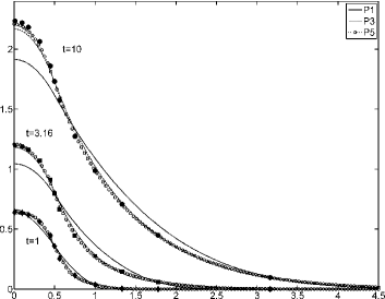
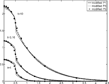
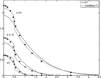
[$P_{N}$ approximations.]           [$D_{N}$ approximations.] [Comparison: $D_{1}$ vs. $P_{1}$ approximations.]           [Comparison: $D_{3}$ vs. $P_{3}$ approximations.]

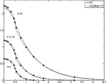
Figure 2: Energy distribution at time $t=1\,s$, $t=3.16\,s$ and $t=10\,s$ for $P_{N}$ and $D_{N}$ approximations of different order.

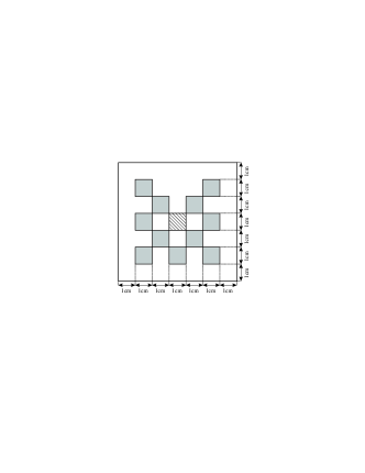
Figure 3: Gray regions and the center area are highly absorbing while white regions are highly scattering. The radiation source is located in the hatched center region.

The thick black symbols mark the benchmark solution at times $t=1\,s$, $t=3.16\,s$ and $t=10\,s$. The other curves are explained in the legend of each plot.

As we can see in Figure 2 and Figure 2, the $P_{N}$ methods as well as the $D_{N}$ approaches lead to solutions that converge for increasing order $N$ to the benchmark solution. But comparing the order of the method that is necessary to reach a specific accuracy shows that the $D_{N}$ approach leads to similar results with less computational effort. Additionally, we see that for small times ($t=1$) both methods perform similarly well. But for large times ($t=10$) the $D_{1}$ solution agrees already very well with the benchmark solution while the $P_{1}$ solution is much further away, especially in the region of the central peak. The solutions of order $5$ in the $D_{N}$ and $P_{N}$ approach (not shown) are almost identical and differ only in a few regions from the benchmark solution.

7.2 Lattice Problem

This is an example with a complicated geometry, taken from [3]. We consider a checkerboard of highly scattering and highly absorbing regions on a lattice core. A graphical representation of the setting is shown in Figure 3. The white regions consist of a purely scattering material with $\kappa=0\,cm^{-1}$ and $\sigma=1\,cm^{-1}$. The eleven gray regions and the central region are purely absorbing with $\kappa=10\,cm^{-1}$ and $\sigma=0\,cm^{-1}$. For the propagation speed we assume $c=1\,cm/s$. At time zero, a source of strength one is turned on in the hatched central region. The computational domain is surrounded on all sides by vacuum boundaries.

The numerical results presented here have been obtained using a finite element discretization with streamline diffusion. We used between 25000 and 400000 bilinear elements. More details on the method can be found in [21].

In Figure 4 we present the energy distribution ($\int_{S^{2}}I(\Omega)d\Omega$) of the radiative field $3.2$ seconds after the radiation source in the center is turned on. The scale is logarithmic ($\log_{10}$). We compare $P_{N}$ methods with $D_{N}$ methods of different order.

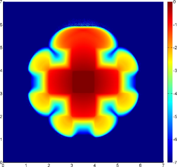
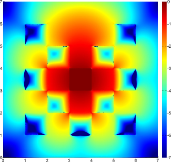
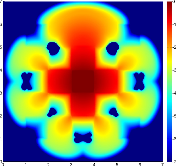
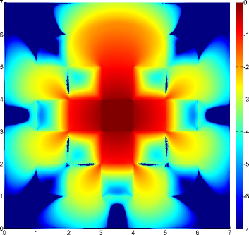
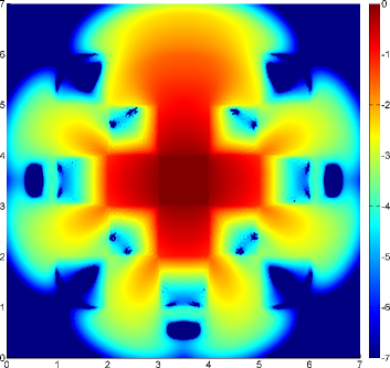
[$P_{1}$]           [$D_{1}$] [$P_{3}$]           [$D_{3}$] [$P_{5}$]           [$D_{5}$]

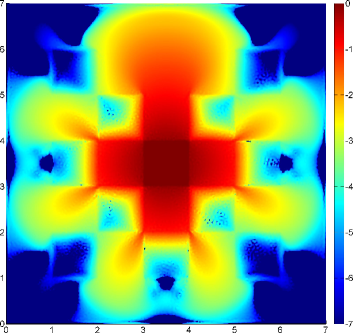
Figure 4: Energy distribution for lattice problem approximated by $P_{N}$ and $D_{N}$ methods of different order presented in a logarithmic scale ($\log_{10}$).

[$P_{7}$]           [$D_{7}$] Energy distribution for lattice problem approximated by $P_{N}$ and $D_{N}$ methods of different order presented in a logarithmic scale ($\log_{10}$). (continued)

The main differences in the solutions can be found in the beams leaking between the corners of the absorbing regions, the shadows behind the absorbing regions and the front of photons escaping from the source region.

As we can see in the resulting figures, for increasing order, both approaches converge to the same solution which for the $P_{7}$ and $D_{7}$ models is almost the same as the one obtained by Monte Carlo simulations in [3]. But the $D_{N}$ model gives much better results for lower order approximations than the $P_{N}$ model. In particular, the front of the escaping photons is tracked much better and the shadows behind the absorbing regions are more visible in lower order $D_{N}$ approaches.

The fact that the front of photons is not captured that well by the $P_{N}$ method is related to the hyperbolic structure of the equations. Especially in the $P_{1}$ model the information can be distributed only with one characteristic speed of $1/\sqrt{3}\,cm/s$. But that is far too slow, compared to the real speed of the photons ($1\,cm/s$). The higher the order $N$ of the $P_{N}$ approximations the more the characteristic speed of the equations approaches the desired one and therefore the front can be tracked much better (see [25]). Due to the additional diffusive term introduced by the deviation approximation into the $D_{N}$ approximation, this effect is not present there.

Appendix A Properties of Spherical Harmonics

Spherical harmonics are used as a set of basis functions for representing functions mapping from the unit sphere into the complex numbers. A good overview on the basics and properties of spherical harmonics can be found in [2]. Here only the most important properties related to moment methods will be recalled.

Since Spherical harmonics act on the unit sphere, a parameterization is needed

$${S^{2}}=\{\Omega\in\mathbb{R}^{3}:\;\Omega=\begin{pmatrix}\sqrt{1-\mu^{2}}\cos\varphi\\ \sqrt{1-\mu^{2}}\sin\varphi\\ \mu\\ \end{pmatrix},\;\varphi\in[0,2\pi],\;\mu\in[-1,1]\}\;.$$ (A.1)

Using these coordinates and the associated Legendre polynomials gives rise to

Definition A.1.

For all $n\in\mathbb{N}_{0}$ and $m\in\{-n,\ldots,n\}$ the function

$$\begin{split}Y^{m}_{n}:\;&{S^{2}}\to\mathbb{C}\\ &(\varphi,\mu)\mapsto(-1)^{m}\sqrt{\frac{2n+1}{4\pi}\frac{(n-m)!}{(n+m)!}}P^{m}_{n}(\mu)e^{im\varphi}\end{split}$$ (A.2)

is called a spherical harmonic function of order $n$ and degree $m$, where the associated Legendre polynomials of order $n$ and degree $m$ are defined from the Legendre polynomials $P_{n}$ as

$$P^{m}_{n}(\mu)=(1-\mu^{2})^{\frac{m}{2}}\frac{d^{m}}{d\mu^{m}}P_{n}(\mu)\qquad n\in\mathbb{N}_{0},\;m=0,\ldots,n\;.$$ (A.3)

If it is clear from the context, the dependence on $\Omega$ will be neglected and we write $Y^{m}_{n}=Y^{m}_{n}(\Omega)$. For indices $m\notin\{-n,\ldots,n\}$ the spherical harmonics are identically zero. For the set of all spherical harmonics we introduce

Definition A.2.

The vector of all spherical harmonics is given by

$${\mathbf{Y}}(\Omega)=\left(Y^{0}_{0}(\Omega),Y^{-1}_{1}(\Omega),Y^{0}_{1}(\Omega),Y^{1}_{1}(\Omega),\ldots\right)^{T}\subset l^{2}\left(L^{2}({S^{2}},\mathbb{C})\right)\;.$$ (A.4)

The spherical harmonics up to order $N$ can be represented by

$${\mathbf{Y}}_{N}(\Omega)=\left(Y^{0}_{0}(\Omega),Y^{-1}_{1}(\Omega),Y^{0}_{1}(\Omega),\ldots,Y^{N-1}_{N}(\Omega),Y^{N}_{N}(\Omega)\right)^{T}\;.$$ (A.5)

Again, if it is clear what we are referring to we neglect the dependence on $\Omega$ and simply write ${\mathbf{Y}}$ and ${\mathbf{Y}}_{N}$.

We use the following properties of spherical harmonics to derive moment models. There is a relation between spherical harmonics and their complex conjugated counterpart

$$Y^{m}_{n}(\Omega)=(-1)^{m}\overline{Y^{-m}_{n}(\Omega)}\;,$$ (A.6)

an addition theorem which leads to a relation between spherical harmonics and Legendre polynomials

$$P_{n}(\Omega\cdot\Omega^{\prime})=\frac{4\pi}{2n+1}\sum_{k=-n}^{n}Y^{k}_{n}(\Omega)\;\overline{Y^{k}_{n}(\Omega^{\prime})}\;,$$ (A.7)

and the recursion relations

$$\begin{split}e^{-i\varphi}\sin\theta\;Y^{m}_{n}&=h_{1}(m,n)Y^{m-1}_{n+1}-l_{1}(m,n)Y^{m-1}_{n-1}\\ e^{i\varphi}\sin\theta\;Y^{m}_{n}&=-h_{2}(m,n)Y^{m+1}_{n+1}+l_{2}(m,n)Y^{m+1}_{n-1}\\ \cos\theta\;Y^{m}_{n}&=h_{3}(m,n)Y^{m}_{n+1}+l_{3}(m,n)Y^{m}_{n-1}\end{split}$$ (A.8)

with the coefficients

$$h_{1}(m,n)=\sqrt{\frac{(n-m+1)(n-m+2)}{(2n+1)(2n+3)}}\quad \quad l_{1}(m,n)=\sqrt{\frac{(n+m)(n+m-1)}{(2n-1)(2n+1)}}$$

$$h_{2}(m,n)=\sqrt{\frac{(n+m+1)(n+m+2)}{(2n+1)(2n+3)}}\quad \quad l_{2}(m,n)=\sqrt{\frac{(n-m)(n-m-1)}{(2n-1)(2n+1)}}$$ (A.9)

$$h_{3}(m,n)=\sqrt{\frac{(n-m+1)(n+m+1)}{(2n+1)(2n+3)}}\quad \quad l_{3}(m,n)=\sqrt{\frac{(n-m)(n+m)}{(2n-1)(2n+1)}}\;.$$

It is easy to see that for the coefficients in (A) it holds

$$\begin{split}h_{1}(m,n)=h_{2}(-m,n)\;,\quad&\quad l_{1}(m,n)=l_{2}(-m,n)\;,\\ h_{3}(m,n)=h_{3}(-m,n)\;,\quad&\quad l_{3}(m,n)=l_{3}(-m,n)\;.\end{split}$$ (A.10)

Using the given recursion relations leads for any vector $\Omega$ on the unit sphere to

$$\Omega Y^{m}_{n}=\begin{pmatrix}\frac{1}{2}\left(h_{1}(m,n)Y^{m-1}_{n+1}-h_{2}(m,n)Y^{m+1}_{n+1}-l_{1}(m,n)Y^{m-1}_{n-1}+l_{2}(m,n)Y^{m+1}_{n-1}\right)\\ \frac{i}{2}\left(h_{1}(m,n)Y^{m-1}_{n+1}+h_{2}(m,n)Y^{m+1}_{n+1}-l_{1}(m,n)Y^{m-1}_{n-1}-l_{2}(m,n)Y^{m+1}_{n-1}\right)\\ h_{3}(m,n)Y^{m}_{n+1}+l_{3}(m,n)Y^{m}_{n-1}\end{pmatrix}.$$ (A.11)

To express the relations (A.11) as matrix–vector multiplications we introduce some new matrices. For $j\in\{1,2,3\}$ the matrices $L_{x_{j}}^{k}\in\mathbb{R}^{2k+1}\times\mathbb{R}^{2k-1}$ and $U_{x_{j}}^{k}\in\mathbb{R}^{2k-1}\times\mathbb{R}^{2k+1}$ are defined as

$$\left(L_{x_{1}}^{k}\right)_{(r,s)} =\begin{cases}-l_{1}(r-k-1,k)&\text{for}\;r=s+2\\ l_{2}(r-k-1,k)&\text{for}\;r=s\\ 0&\text{otherwise}\end{cases}\;,$$ (A.12a)

$$\left(L_{x_{2}}^{k}\right)_{(r,s)} =\begin{cases}-l_{1}(r-k-1,k)&\text{for}\;r=s+2\\ -l_{2}(r-k-1,k)&\text{for}\;r=s\\ 0&\text{otherwise}\end{cases}\;,$$ (A.12b)

$$\left(L_{x_{3}}^{k}\right)_{(r,s)} =\begin{cases}l_{3}(r-k-1,k)&\text{for}\;r=s+1\\ 0&\text{otherwise}\end{cases}$$ (A.12c)

and

$$\left(U_{x_{1}}^{k}\right)_{(r,s)} =\begin{cases}h_{1}(r-k,k-1)&\text{for}\;r=s\\ -h_{2}(r-k,k-1)&\text{for}\;r=s-2\\ 0&\text{otherwise}\end{cases}\;,$$ (A.13a)

$$\left(U_{x_{2}}^{k}\right)_{(r,s)} =\begin{cases}h_{1}(r-k,k-1)&\text{for}\;r=s\\ h_{2}(r-k,k-1)&\text{for}\;r=s-2\\ 0&\text{otherwise}\end{cases}\;,$$ (A.13b)

$$\left(U_{x_{3}}^{k}\right)_{(r,s)} =\begin{cases}h_{3}(r-k,k-1)&\text{for}\;r=s-1\\ 0&\text{otherwise}\end{cases}\;.$$ (A.13c)

We used the definitions of $l_{i}(\cdot,\cdot)$ and $h_{i}(\cdot,\cdot)$ from (A). The resulting matrices have only two (or for $L_{x_{3}}^{k}$ and $U_{x_{3}}^{k}$ only one) diagonals that do not vanish. Their structure is

$$\begin{split}&U_{x_{1}}^{k}=\begin{pmatrix}h_{1}&0&-h_{2}&&\\ &h_{1}&0&-h_{2}&\\ &&\ddots&\ddots&\ddots\\ \end{pmatrix}\qquad U_{x_{2}}^{k}=\begin{pmatrix}h_{1}&0&h_{2}&&\\ &h_{1}&0&h_{2}&\\ &&\ddots&\ddots&\ddots\\ \end{pmatrix}\\ &\qquad\qquad\qquad\qquad\qquad U_{x_{3}}^{k}=\begin{pmatrix}0&h_{3}&0&&\\ &0&h_{3}&0&\\ &&\ddots&\ddots&\ddots\\ \end{pmatrix}\end{split}$$ (A.14)

$$L_{x_{1}}^{k}=\begin{pmatrix}l_{2}&&\\ 0&l_{2}&\\ -l_{1}&0&\ddots\\ &-l_{1}&\ddots\\ &&\ddots\\ \end{pmatrix}\qquad L_{x_{2}}^{k}=\begin{pmatrix}-l_{2}&&\\ 0&-l_{2}&\\ -l_{1}&0&\ddots\\ &-l_{1}&\ddots\\ &&\ddots\\ \end{pmatrix}\qquad L_{x_{3}}^{k}=\begin{pmatrix}0&&\\ l_{3}&0&\\ 0&l_{3}&\ddots\\ &0&\ddots\\ &&\ddots\\ \end{pmatrix}$$ (A.15)

In this representation we neglected the dependence of the coefficients $l_{1},h_{1},\ldots$ on the order of the spherical harmonics. These relations can be found in (A.12) and (A.13).

The matrices can be combined to larger matrices $\hat{L}_{x_{j}}^{N}$ and $\hat{U}_{x_{j}}^{N}$ in the following way

$$\hat{L}_{x_{j}}^{N}=\begin{pmatrix}0&&&&\\ L_{x_{j}}^{1}&0&&&\\ &L_{x_{j}}^{2}&\ddots&&\\ &&&\ddots&\\ &&&L_{x_{j}}^{N}&0\\ \end{pmatrix}\quad\text{and}\quad\hat{U}_{x_{j}}^{N}=\begin{pmatrix}0&U_{x_{j}}^{1}&&&\\ &&U_{x_{j}}^{2}&&\\ &&\ddots&&\\ &&&\ddots&U_{x_{j}}^{N}\\ &&&&0\\ \end{pmatrix}\;.$$ (A.16)

Additionally we introduce the factor

$$\gamma_{j}=\begin{cases}\frac{1}{2}&\text{for}\quad j=1\\ \frac{i}{2}&\text{for}\quad j=2\\ 1&\text{for}\quad j=3\end{cases}$$ (A.17)

and the unit vector

$$\mathbb{R}^{(N+1)^{2}}\ni{\mathbf{e}}^{N}_{(m,n)}=(0,\ldots,0,1,0,\ldots,0)^{T}$$ (A.18)

which is one only in the component that is related to the spherical harmonic $Y^{m}_{n}$ in the vector ${\mathbf{Y}}_{N}$ such that $\left({\mathbf{e}}^{N}_{(m,n)}\right)^{T}{\mathbf{Y}}_{N}=Y^{m}_{n}$. Then, for $n\in\{0,\ldots,N\}$ and $m\in\{-n,\ldots,n\}$, we can write

$$\Omega_{j}Y^{m}_{n}=\gamma_{j}\left(\left({\mathbf{e}}^{N}_{(m,n)}\right)^{T}\hat{L}_{x_{j}}^{N}{\mathbf{Y}}_{N}+\left({\mathbf{e}}^{N+1}_{(m,n)}\right)^{T}\hat{U}_{x_{j}}^{N+1}{\mathbf{Y}}_{N+1}\right)\;.$$ (A.19)

Lemma A.3.

For the matrices $\hat{L}_{x_{j}}^{N}$ and $\hat{U}_{x_{j}}^{N}$ hold the relations

$$\left(\hat{L}_{x_{1}}^{N}\right)^{T}=\hat{U}_{x_{1}}^{N}\;,\qquad\left(\hat{L}_{x_{2}}^{N}\right)^{T}=-\hat{U}_{x_{2}}^{N}\;,\qquad\left(\hat{L}_{x_{1}}^{N}\right)^{T}=\hat{U}_{x_{1}}^{N}\;.$$ (A.20)

Appendix B Treatment of Scattering and Absorption operators in moment methods

The radiative transfer equation contains a scattering component

$$({\mathcal{S}}I)(t,x,\Omega)=\frac{\sigma}{4\pi}\int_{S^{2}}\Phi(x,\Omega\cdot\Omega^{\prime})I(t,x,\Omega^{\prime})\,d\Omega^{\prime}$$ (B.1)

with a normalized scattering kernel $\Phi$. This scattering kernel can be rather complicated. Several theories have been developed to approximate realistic kernels. The first who established an approach was Mie [24]. However, due to the complexity of his theory, several simplified approximations have been developed, e.g. the Henyey-Greenstein (HG) kernel [28] or the SAM (simplified approximate Mie) approach [16].

To deal with the scattering kernel in moment methods, it is very common to rewrite it into a series expansion based on Legendre polynomials

$$\Phi(x,\mu)=\sum_{j=0}^{\infty}\frac{2j+1}{2}\sigma_{j}(x)P_{j}(\mu)\;.$$ (B.2)

This leads to

$${\mathcal{S}}I(\Omega)=\frac{\sigma}{2}\sum_{l=0}^{\infty}\sum_{k=-l}^{l}\sigma_{l}{\mathbf{I}}^{k}_{l}Y^{k}_{l}(\Omega)$$ (B.3)

and

$$\textswab{m}^{r}_{s}{\mathcal{S}}I(\Omega)=\frac{\sigma}{2}\sum_{l=0}^{\infty}\sum_{k=-l}^{l}\sigma_{l}{\mathbf{I}}^{k}_{l}\left(\textswab{m}^{r}_{s}Y^{k}_{l}(\Omega)\right)=\frac{\sigma}{2}\sum_{l=0}^{\infty}\sum_{k=-l}^{l}\sigma_{l}{\mathbf{I}}^{k}_{l}\delta^{k}_{r}\delta^{l}_{s}=\frac{\sigma}{2}\sigma_{s}{\mathbf{I}}^{r}_{s}\;.$$ (B.4)

For the total absorption and scattering operator we get

$$({\mathcal{K}}I)(\Omega)=\sum_{l=0}^{\infty}\sum_{k=-l}^{l}\left(\kappa+\sigma-\frac{\sigma}{2}\sigma_{l}\right){\mathbf{I}}^{k}_{l}Y^{k}_{l}(\Omega)=:\sum_{l=0}^{\infty}\sum_{k=-l}^{l}\tilde{\sigma}_{l}{\mathbf{I}}^{k}_{l}Y^{k}_{l}(\Omega)$$ (B.5)

It is obvious that the inverse operator is

$$({\mathcal{K}}^{-1}I)(\Omega)=\sum_{l=0}^{\infty}\sum_{k=-l}^{l}\frac{1}{\kappa+\sigma-\frac{\sigma}{2}\sigma_{l}}{\mathbf{I}}^{k}_{l}Y^{k}_{l}(\Omega)\;.$$ (B.6)

and thus

$$\textswab{m}^{r}_{s}({\mathcal{K}}^{-1}I)(\Omega)=\frac{1}{\kappa+\sigma-\frac{\sigma}{2}\sigma_{s}}{\mathbf{I}}^{r}_{s}.$$ (B.7)

References

[1]
A. M. Anile, S. Pennisi, and M. Sammartino, A thermodynamical approach to
Eddington factors, J. Math. Phys. 32 (1991), 544–550.
[2]
George Arfken, Mathematical methods for physicists, 2 ed., Academic
Press, 1970.
[3]
T.A. Brunner and J. P. Holloway, Two-dimensional time dependent Riemann
solvers for neutron transport, Journal of Computational Physics 210
(2005), 386–399.
[4]
S. Chandrasekhar, On the radiative equilibrium of a stellar atmosphere,
Astrophysical Journal 99 (1944), 180.
[5]
R. Dautray and J. L. Lions, Mathematical analysis and numerical methods
for science and technology (v.6), Springer, Paris, 1993.
[6]
B. Davison, Neutron transport theory, Oxford University Press, 1958.
[7]
B. Dubroca and J. L. Feugeas, Entropic moment closure hierarchy for the
radiative transfer equation, C. R. Acad. Sci. Paris Ser. I 329
(1999), 915–920.
[8]
M. Frank, C.D. Hauck, and C.D. Levermore, Boundary conditions for moment
closures, in preparation, 2009.
[9]
M. Frank and B. Seibold, Optimal prediction for radiative transfer: A new
perspective on moment closure, (2009), submitted.
[10]
E. M. Gelbard, Simplified spherical harmonics equations and their use in
shielding problems, Tech. Report WAPD-T-1182, Bettis Atomic Power
Laboratory, 1961.
[11]
E. W. Larsen, G. Thömmes, A. Klar, M. Seaïd, and T. Götz,
Simplified approximations to the equations of radiative heat
transfer in glass, J. Comput. Phys. 183 (2002), 652–675.
[12]
C. D. Levermore, Relating Eddington factors to flux limiters, J.
Quant. Spectrosc. Radiat. Transfer 31 (1984), 149–160.
[13]
, Moment closure hierarchies for kinetic theories, J. Stat. Phys.
83 (1996), 1021–1065.
[14]
C. D. Levermore, Transition regime models for radiative transport,
presentation at IPAM: Grand challenge problems in computational
astrophysics workshop on transfer phenomena, 2005.
[15]
, Moment closures for radiative transport, in preparation, 2009.
[16]
P. Liu, A new phase function approximation to Mie scattering for
radiative transport equations, Phys. Med. Biol. 39 (1994),
1025–1036.
[17]
G. N. Minerbo, Maximum entropy Eddington factors, J. Quant. Spectrosc.
Radiat. Transfer 20 (1978), 541–545.
[18]
I. Pascucci, S. Wolf, J. Steinacker, C. P. Dullemonda, Th. Henning,
G. Niccolini, P. Woitke, and B. Lopez, The continuum radiative
transfer problem, Astronomy & Astrophysics 417 (2004), 793–805.
[19]
G. C. Pomraning, Asymptotic and variational derivations of the simplified
equations, Ann. Nuclear Energy 20 (1993), 623.
[20]
S. Rosseland, Theoretical astrophysics: Atomic theory and the analysis of
stellar atmospheres and envelopes, Clarendon Press, 1936.
[21]
M. Schäfer, Moment methods for radiative transfer - modeling,
simulation and optimization, Ph.D. thesis, University of Kaiserslautern,
2008, ISBN 978-3-89963-717-5.
[22]
B. Seibold and M. Frank, Optimal prediction for moment models: crescendo
diffusion and reordered equations, Continuum Mech. Thermodyn. (2009), to
appear.
[23]
J. Steinacker, A. Bacmann, and T. Henning, Ray tracing for complex
astrophysical high-opacity structures, The Astrophysical Journal
645 (2006), 920–927.
[24]
J. A. Stratton, Electromagnetic theory, McGraw-Hill New York, 1941.
[25]
H. Struchtrup, On the number of moments in radiative transfer problems,
Ann. Phys. (N.Y.) 266 (1998), 1–26.
[26]
B. Su and G.L. Olson, An analytical benchmark for non-equilibrium
radiative transfer in an isotropically scattering medium, Ann. Nucl. Energy
24 (1997), no. 13, 1035–1055.
[27]
G. Thömmes, Radiative heat transfer equations for glass cooling
problems: Analysis and numerics, Ph.D. thesis, TU Darmstadt, 2002.
[28]
H. C. Van de Hulst, Multiple light scattering: Tables, formulas and
applications, New York: Academic Press, 1980.
[29]
S. Wolf, Inverse raytracing based on the Monte-Carlo method,
Astronomy & Astrophysics 379 (2001), 690–696.
[30]
S. Wolf, Th. Henning, and B. Stecklum, Multidimensional self-consistent
radiative transfer simulations based on the Monte-Carlo method,
Astronomy & Astrophysics 349 (1999), 839–850.