Simultaneously Sparse Solutions to Linear Inverse Problems with Multiple System Matrices and a Single Observation Vector††thanks: This document is a manuscript from July 21, 2008, unchanged except for updated references. The content appears in the first author’s September 2008 PhD thesis.
Abstract
A linear inverse problem is proposed that requires the determination of multiple unknown signal vectors. Each unknown vector passes through a different system matrix and the results are added to yield a single observation vector. Given the matrices and lone observation, the objective is to find a simultaneously sparse set of unknown vectors that solves the system. We will refer to this as the multiple-system single-output (MSSO) simultaneous sparsity problem. This manuscript contrasts the MSSO problem with other simultaneous sparsity problems and conducts a thorough initial exploration of algorithms with which to solve it.
Seven algorithms are formulated that approximately solve this NP-Hard problem. Three greedy techniques are developed (matching pursuit, orthogonal matching pursuit, and least squares matching pursuit) along with four methods based on a convex relaxation (iteratively reweighted least squares, two forms of iterative shrinkage, and formulation as a second-order cone program). While deriving the algorithms, we prove that seeking a single sparse complex-valued vector is equivalent to seeking two simultaneously sparse real-valued vectors. In other words, single-vector sparse approximation of a complex vector readily maps to the MSSO problem, increasing the applicability of MSSO algorithms.
The algorithms are evaluated across three experiments: the first and second involve sparsity profile recovery in noiseless and noisy scenarios, respectively, while the third deals with magnetic resonance imaging radio-frequency excitation pulse design. For sparsity profile recovery, the iteratively reweighted least squares and second-order cone programming techniques outperform the greedy algorithms, whereas in the magnetic resonance imaging pulse design experiment, the greedy least squares matching pursuit algorithm exhibits superior performance. Overall, each algorithm is found to have particular merits and weaknesses, e.g., the iterative shrinkage techniques converge slowly, but because they update only a subset of the overall solution per iteration rather than all unknowns at once, they are useful in cases where attempting the latter is prohibitive in terms of system memory.
keywords:
sparse approximation, simultaneous sparse approximation, multiple unknown vectors, greedy pursuit, iteratively reweighted least squares, iterative shrinkage, second-order cone programming1 Introduction
In this work we propose a linear inverse problem that requires a simultaneously sparse set of vectors as the solution, i.e., a set of vectors where only a small number of each vector’s entries are nonzero, and where the vectors’ sparsity profiles (the locations of the nonzero entries) are equivalent (or are promoted to be equivalent with an increasing penalty given otherwise).
Prior work on simultaneously sparse solutions to linear inverse problems involves multiple unknown vectors, a single system matrix, and a host of observation vectors; the th observation vector arises by multiplying the single system matrix with the th unknown vector [7, 33, 49, 47]. Given the observation vectors and system matrix, one seeks out a simultaneously sparse set of unknown vectors that (approximately) solves the overall system. We will refer to this as the single-system multiple-output (SSMO) simultaneous sparsity problem.
Here we study a problem that is somewhat similar yet different from the aforementioned one. This multiple-system single-output (MSSO) simultaneous sparsity problem still consists of multiple unknown vectors, but now each such vector is passed through a different system matrix and the outputs of the various system matrices undergo a linear combination, yielding only one observation vector. Given the matrices and lone observation, one must find a simultaneously sparse set of vectors that (approximately) solves the system. To date, this problem has been explored in a magnetic resonance imaging (MRI) radio-frequency (RF) excitation pulse design context [52, 51, 53], but it may also have applications to source localization using sensor arrays [26, 30] and signal denoising [11, 4, 20, 16].
Both SSMO and MSSO arise as generalizations of the single-system single-output (SSSO) sparse approximation problem, where there is one known observation vector, a known system matrix, and the solution one seeks is a single sparse unknown vector [23, 4, 40]. Several styles of algorithms have been posed to solve the SSSO problem, such as forward-looking greedy pursuit [34, 35, 3, 10, 6], iteratively reweighted least squares (IRLS) [28] (e.g., FOCUSS [23]), iterative shrinkage [14, 8, 15, 16], and second-order cone programming (SOCP) [2, 33]. Many of these have been extended to the SSMO problem [7, 33, 49, 47].
In this manuscript, we propose three forward-looking greedy techniques—matching pursuit (MP) [34], orthogonal matching pursuit (OMP) [35, 3, 6], and least squares matching pursuit (LSMP) [6]—and also develop IRLS-based, shrinkage-based, and SOCP-based algorithms to solve the MSSO simultaneous sparsity problem. We then evaluate the performance of the algorithms across three experiments: the first and second involve sparsity profile recovery in noiseless and noisy scenarios, respectively, while the third deals with MRI RF excitation pulse design.
The structure of this paper is as follows: in Sec. 2, we provide background information about ordinary (SSSO) sparse approximation and SSMO sparse approximation. In Sec. 3, we formulate the MSSO problem. Seven algorithms for solving the problem are then posed in Sec. 4, while the details and results of the three numerical experiments appear in Sec. 5. Section 6 highlights the strengths and weaknesses of the algorithms and presents ideas for future work. Concluding remarks are given in Sec. 7.
2 Background
2.1 Single-System Single-Output (SSSO) Sparse Approximation
Consider a linear system of equations , where , , , and and are known. It is common to use the Moore-Penrose pseudoinverse of , denoted , to determine as an (approximate) solution to the system of equations. When is in the range of , is the solution that minimizes , the Euclidean or norm of . When is not in the range of , no solution exists; minimizes among the vectors that minimize .
When a sparse solution is desired, it is necessary for the analogue to to have only a small fraction of its entries differ from zero. We are faced with a sparse approximation problem of the form
| (1) |
where denotes the number of nonzero elements of a vector. The subset of where there are nonzero entries in is called the sparsity profile. For general , solving (1) essentially requires a search over up to nonempty sparsity profiles. The problem is thus computationally infeasible except for very small systems of equations (e.g., even for , one may need to search 1,073,741,823 subsets). Formally, the problem is NP-Hard [9, 35].
For problems where (1) is intractable, a large body of work supports a greedy search over the columns of to seek out a small subset of columns that, when weighted and linearly combined, yields a result that is close to in the sense, along with a sparse [34, 35, 3, 10, 6].
A second body of research supports the relaxation of (1) to find a sparse [4]:
| (2) |
This is a convex optimization and thus may be solved efficiently [2]. The solution of (2) does not always match the solution of (1)—if it did, the intractability of (1) would be contradicted—but certain conditions on guarantee a proximity of their solutions [12, 13, 48]. Note that (2) applies an norm to , but an norm (where ) may also be used to promote sparsity [23, 4]; this leads to a non-convex problem and will not considered in this paper.
The optimization
| (3) |
has the same set of solutions as (2). The first term of (3) keeps residual error down, whereas the second promotes sparsity of [43, 4]. As the control parameter, , is increased from zero to infinity, the algorithm yields sparser solutions and the residual error increases; sparsity is traded off with residual error. In this paper we shall hereafter use formulation (3) and its analogues rather than (2).
It is important to understand that a problem of the form (3) may arise as a proxy for (1) or as the inherent problem of interest. For example, in a Bayesian estimation setting, (3) yields the maximum a posteriori probability estimate of from when the observation model involves and Gaussian noise and the prior on is Laplacian. Similar statements can be made about the relaxations of the simultaneous sparse approximation problems posed in the following sections.
2.2 Single-System Multiple-Output (SSMO) Simultaneous Sparse Approximation
In SSMO, we have observation vectors (“snapshots”), all of which arise from the same system matrix:
| (4) |
where is known for along with . In this scenario, we want to constrain the number of positions at which any of the s are nonzero. Thus we seek approximate solutions in which the s are not only sparse, but the union of their sparsity patterns is small; that is, a simultaneously sparse set of vectors is desired [33, 47]. Unfortunately, optimal approximation with a simultaneous sparsity constraint is even harder than (1).
Extending single-vector sparse approximation greedy techniques is one way to find an approximate solution [7, 49]. Another approach is to extend the relaxation (3) as follows:
| (5) |
where , , is the Frobenius norm, and
| (6) |
i.e., is the norm of the norms of the rows of the matrix.111Although here we have applied an norm to the row energies of , an norm (where ) could be used in place of the norm if one is willing to deal with a non-convex objective function. Further, an norm (where ) rather than an norm could be applied to each row of because the purpose of the row operation is to collapse the elements of the row into a scalar value without introducing a sparsifying effect. This latter operator is a simultaneous sparsity norm: it penalizes the program (produces large values) when the columns of have dissimilar sparsity profiles [33]. Fixing to a sufficiently large value and solving this optimization yields simultaneously sparse s. For , (5) collapses to the base case of (3). Given the convex objective function in (5), one may then attempt to find a solution that minimizes the objective using an IRLS-based [7], or SOCP-based [33] approach. A formal analysis of the minimization of the convex objective may be found in [47].
3 Multiple-System Single-Output (MSSO) Simultaneous Sparse Approximation
We outline the MSSO problem in a style analogous to that of SSMO systems in (4, 5) and then pose a second formulation that is useful for deriving several algorithms in Sec. 4.
3.1 MSSO Problem Formulation
Consider the following system:
| (7) |
where and the are known. Unlike the SSMO problem, there is now only one observation and different system matrices. Here we again desire an approximate solution where the s are simultaneously sparse; formally,
| (8) |
This is, of course, harder than the SSSO problem and thus NP-Hard. To keep the problem as general as possible, there are no constraints on the values of , , or , i.e., there is no explicit requirement that the system be overdetermined or underdetermined. Further, we have used complex-valued rather than real-valued variables.
In the first half of Sec. 4, we will pose three approaches that attempt to solve the MSSO problem (8) in a greedy fashion. Another approach to solve the problem is to apply a relaxation similar to (3, 5):
| (9) |
where and are the same as in (5) and (6), respectively. In the second half of Sec. 4, we will outline four algorithms for solving this relaxed problem. By setting , (9) collapses to the base case of (3).
3.2 Alternate Formulation of the MSSO Problem
In several upcoming derivations, it will be useful to view the system from a different standpoint. To begin, we construct several new variables that are simply permutations of the s and s. First we define new matrices:
| (10) |
where is the th column of . Next we construct new vectors:
| (11) |
where is the th element of and is the transpose operation. Given the s and s, we now pose the following system:
| (12) |
Due to (10, 11), the system in (12) is equivalent to the one in (7). The relationship between the s and s implies that if we desire to find a set of simultaneously sparse s to solve (7), we should seek out a set of s where many of the s equal an all-zeros vector, , but a few s are high in energy (typically with all elements being nonzero). This claim is apparent if we consider the fact that is equal to the transpose of , and that the s are only simultaneously sparse when is sufficiently small.
Continuing with this alternate formulation, and given our desire to find a solution where most of the s are all-zero vectors and a few are dense, we relax the problem as follows:
| (13) |
Fixing to a sufficiently large value and solving this optimization yields many low-energy s (each close to ), along with several dense high-energy s. Further, because is equivalent to , this means (13) is equivalent to (9), and thus just like (9), the approach in (13) finds a set of simultaneously sparse s.
3.3 Differences between the SSMO and MSSO Problems
In the SSMO problem, we see from (4) that there are many different s and a single . The ratio of unknowns to knowns always equals regardless of the number of observations, . A large when solving SSMO is actually beneficial because the simultaneous sparsity of the underlying s becomes more exploitable; empirical evidence of improved sparsity profile recovery with increasing may be found in both [7] and [33].
In contrast, we see from (7) that in the MSSO problem there is a single and many different s. Here the ratio of unknowns to knowns is no longer constant with respect to ; rather it is equal to . We will show in Sec. 5 that as increases, the underlying simultaneous sparsity of the s is not enough to combat the increasing number of unknowns, and that for large , correctly identifying the sparsity profile of the underlying unknown s is a daunting task.
4 Proposed Algorithms
We now derive algorithms to (approximately) solve the MSSO problem defined in Sec. 3.
4.1 Matching Pursuit (MP)
To begin, we extend the single-vector case of matching pursuit [34] to an MSSO context. The classic MP technique first finds the column of the system matrix that best matches with the observed vector and then removes from the observation vector the projection of this chosen column. It proceeds to select a second column of the system matrix that best matches with the residual observation, and continues doing so until either columns have been chosen (as specified by the user) or the residual observation ends up as a vector of all zeros. This algorithm is fast and computationally-efficient because the best-matching column vector during each iteration is determined simply by calculating the inner product of each column vector with the residual observation and ranking the resulting inner product magnitudes.
Now let us consider the MSSO system as posed in (12). In the first iteration of standard MP, we seek out the single column of the system matrix that can best represent . But in the MSSO context, we need to seek out which of the matrices can be best used to represent when the columns of undergo an arbitrarily-weighted linear combination. The key difference here is that on an iteration-by-iteration basis, we are no longer deciding which column vector best represents the observation, but which matrix does so. The intuition behind this approach is that ideal solutions should consist of only a few dense s and many all-zeros s. For the th iteration of the algorithm, we need to select the proper index by solving:
| (14) |
where is the index that will be selected and is the current residual observation. For fixed , the solution to the inner minimization is obtained via the pseudoinverse, , yielding
| (15) |
where is the Hermitian transpose. From (15) we see that, analogously to standard MP, choosing the best index for iteration involves computing and ranking a series of inner-product-like quadratic terms.
Algorithm 1 outlines the entire procedure. After iterations, one obtains (of cardinality ), a set indicating the chosen matrices. The weights to apply to each chosen matrix (i.e., the corresponding s) are obtained via a finalization step; they are the best weightings in the residual error sense with which to linearly combine the columns of the chosen matrices to best match the observation . Since total matrices end up being chosen by the process, there is no penalty in retuning the associated vectors because they are allowed to be dense. The other s (and corresponding s) are not used.222From the perspective of s and s in (7), Algorithm 1 determines weights to place along only rows of (leaving the other rows zeroed out) that still yields a good approximation of in the residual error sense. It is seeking out the best rows of which, when densely filled, yield a sound approximation of .
One property of note is that if , Algorithm 1 stops after one iteration. This is because in this case is simply an identity matrix for all , and thus any one of the s is enough to represent exactly when its columns are properly weighted and linearly combined.
Task: greedily choose up to of the s
to best represent via .
Data and Parameters: and are given.
iterations.
Precompute: , for .
Initialize: Set , , , .
Iterate: Set and apply:
-
.
-
if thenelseend if
-
.
-
. Terminate loop if or . ends with elements.
Compute Weights: , unstack into ; set remaining s to .
4.2 Orthogonal Matching Pursuit (OMP)
In single-vector MP, the residual always ends up orthogonal to the th column of the system matrix, but as the algorithm continues iterating, there is no guarantee the residual remains orthogonal to column or is minimized in the least-squares sense with respect to the entire set of chosen column vectors (indexed by ). Furthermore, iterations of single-vector MP do not guarantee different columns will be selected. Single-vector OMP is an extension to MP that attempts to mitigate these problems by improving the calculation of the residual vector. During the th iteration of single-vector OMP, column is chosen exactly as in MP (by ranking the inner products of the residual vector with the various column vectors), but the residual vector is updated by accounting for all columns chosen up through iteration rather than simply the last one [35, 6].
To extend OMP to the MSSO problem, we choose matrix during iteration as in MSSO MP and then in the spirit of single-vector OMP compute the new residual as follows:
| (16) |
where and is the best choice of that minimizes the residual error . That is, to update the residual we now employ all chosen matrices, weighting and combining them to best represent in the least-squares sense, yielding an that is orthogonal to the columns of (and thus orthogonal to ), which has the benefit of ensuring that OMP will select a new matrix at each step.
Algorithm 2 describes the OMP algorithm; the complexity here is moderately greater than that of MP because the pseudoinversion of an matrix is required during each iteration .
Task: greedily choose up to of the s
to best represent via .
Data and Parameters: and are given.
iterations.
Precompute: , for .
Initialize: Set , , , .
Iterate: Set and apply:
-
.
-
-
-
.
-
. Terminate loop if or . ends with elements.
Compute Weights: , unstack into ; set remaining s to .
4.3 Least Squares Matching Pursuit (LSMP)
Beyond OMP there exists a greedy algorithm with an even greater computational complexity known as LSMP. In single-vector LSMP, one solves least squares minimizations during iteration in order to determine which column of the system matrix may be used to best represent [6].
Thus to extend LSMP to MSSO systems, we must ensure that during iteration we account for the previously chosen matrices when choosing the th one to best construct an approximation to . Specifically, index is selected as follows:
| (17) |
where is the set of indices chosen up through iteration , , , and . For fixed , the solution of the inner iteration is ; it is this step that ensures the residual observation error will be minimized by using all chosen matrices. Substituting into (17) and simplifying the expression yields
| (18) |
where .
Algorithm 3 describes the LSMP method. The complexity here is much greater than that of OMP because pseudoinversions of an matrix are required during each iteration . Furthermore, the dependence of on both and makes precomputing all such matrices infeasible in most cases. One way to decrease computation and runtime might be to extend the projection-based recursive updating scheme of [6] to MSSO LSMP.
Task: greedily choose of the s
to best represent via .
Data and Parameters: and are given.
iterations.
Initialize: Set , , .
Iterate: Set and apply:
-
, where
-
-
-
. Terminate loop if or . ends with elements.
Compute Weights: , unstack into ; set remaining s to .
4.4 Iteratively Reweighted Least Squares (IRLS)
Having posed three greedy approaches for solving the MSSO problem, we now turn our attention toward minimizing (13), the relaxed objective function. Here, the regularization term is used to trade off simultaneous sparsity with residual observation error.
One way to minimize (13) is to use an IRLS-based approach [28]. To begin, consider manipulating the right-hand term of (13) as follows:
| (19) |
where ∗ is the complex conjugate of a scalar, is a real-valued diagonal matrix whose diagonal elements each equal , and is some small non-negative value introduced to mitigate poor conditioning of the s. If we fix by computing it using some prior estimate of , then the right-hand term of (13) becomes a quadratic function and (13) transforms into a Tikhonov optimization [44, 45]:
| (20) |
Finally, by performing a change of variables and exploiting the properties of , we can convert (20) into an expression that may be minimized using the robust and reliable conjugate-gradient (CG) least-squares solver LSQR [38, 37], so named because it applies a QR decomposition [22] when solving the system in the least-squares sense. LSQR works better in practice than several other CG methods [1] because it restructures the input system via the Lanczos process [31] and applies a Golub-Kahan bidiagonalization [21] prior to solving it.
To apply LSQR to this problem, we first construct as the element-by-element square-root of the diagonal matrix and then take its inverse to obtain . Defining and , (20) becomes:
| (21) |
This problem may be solved directly by simply providing , , and to the LSQR package because LSQR is formulated to solve the exact problem in (21). Calling LSQR with these variables yields , and the solution is backed out via .
Algorithm 4 outlines how one may iteratively apply (21) to attempt to find a solution that minimizes the original cost function, (13). The technique iterates until the objective function decreases by less than or the maximum number of iterations, , is exceeded. The initial solution estimate is obtained via pseudoinversion of (an all-zeros initialization would cause to be poorly conditioned). A line search is used to step between the prior solution estimate and the upcoming one; this improves the rate of convergence and ensures the objective decreases at each step. This method is global in the sense that all unknowns are being estimated concurrently per iteration.
Task: Minimize using an iterative scheme.
Data and Parameters: , , , , and are given.
Initialize: Set and
(or e.g. ).
Iterate: Set and apply:
Finalize: Unstack the last solution into .
4.5 Row-by-Row Shrinkage (RBRS)
The proposed IRLS technique solves for all unknowns during each iteration, but this is cumbersome when is large. An alternative approach is to apply an inner loop that fixes and then iteratively tunes while holding the other s () constant; thus only (rather than ) unknowns need to be solved for during each inner iteration.
This idea inspires the RBRS algorithm. The term “row-by-row” is used because each corresponds to row of the matrix in (9), and “shrinkage” is used because the energy of most of the s will essentially be “shrunk” (to some extent) during each inner iteration: when is sufficiently large and many iterations are undertaken, many s will be close to all-zeros vectors and only several will be dense and high in energy.
4.5.1 RBRS for real-valued data
Assume and the s of (13) are real-valued. We now seek to minimize the function by extending the single-vector sequential shrinkage technique of [15] and making modifications to (13). Assume we have prior estimates of through , and that we now desire to update only the th vector while keeping the other fixed. The shrinkage update of is achieved via:
| (22) |
where forms an approximation of using the prior solution coefficients, but discards the component contributed by the original th vector, replacing the latter via an updated solution vector, . The left-hand term promotes a solution that keeps residual error down, whereas the right-hand term penalizes s that contain nonzeros. It is crucial to note that the right-hand term does not promote the element-by-element sparsity of ; rather, it penalizes the overall energy of , and thus both sparse and dense s are penalized equally if their overall energies are the same.
One way to solve (22) is to take its derivative with respect to and find such that the derivative equals . By doing this and shuffling terms, and assuming we have an initial estimate of , we may solve for iteratively:
| (23) |
where , is a identity matrix, and is a small value that avoids ill-conditioned results.333Eq. (23) consists of a direct inversion of a matrix, which is acceptable in this paper because all experiments involve . If is large, (23) could be solved via a CG technique (e.g., LSQR). By iterating on (23) until (22) changes by less than , we arrive at a solution to (22), , and this then replaces the prior solution vector, . Having completed the update of the th vector, we proceed to update the rest of the vectors, looping this outer process times or until the main objective function, (13), changes by less than . Algorithm 5 details the entire procedure; unlike IRLS, here we essentially repeatedly invert matrices to pursue a row-by-row solution, rather than matrices to pursue a solution that updates all rows per iteration.
Task: Minimize using an iterative scheme when all data is real-valued.
Data and Parameters: , , (), , , , and are given.
Initialize: Set and
(or e.g. ), unstack into .
Iterate: Set and apply:
Finalize: If was large enough, several s should be dense and others close to .
4.5.2 Extending RBRS to complex-valued data
If (13) contains complex-valued terms, we may structure the row-by-row updates as in (22), but because the derivative of the objective function in (22) is more complicated due to the presence of complex-valued terms, the simple update equation given in (23) is no longer applicable. One way to overcome this problem is to turn the complex-valued problem into a real-valued one.
Let us create several real-valued expanded vectors:
| (24) |
as well as real-valued expanded matrices:
| (25) |
Due to the structure of (24, 25) and the fact that equals , the following optimization is equivalent to (13):
| (26) |
This means we may apply RBRS to complex-valued scenarios by substituting the s for the s and s for the s in (22, 23) and Algorithm 5. [Eq. (23) becomes an applicable update equation because (22) will consist of only real-valued terms and the derivative calculated earlier is again applicable.] Finally, after running the algorithm to obtain finalized s, we may simply restructure them into complex s.
4.6 Column-by-Column Shrinkage (CBCS)
Here we propose a dual of RBRS—a technique that sequentially updates the columns of (i.e., the s) in (7, 9) rather than its rows (the s). Interestingly, we will show that this approach yields a separable optimization and reduces the overall problem to simply repeated element-by-element shrinkages of each .
4.6.1 CBCS for real-valued data
Assume the s, s, and in (9) are real-valued and that we have prior estimates of the s. Let us consider updating the th vector while keeping the other fixed. This reduces (9) to
| (27) |
where will be the update of , and and are as follows:
| (28) |
and
| (29) |
If the s were not present, (27) would reduce to the standard problem iterated shrinkage is intended to solve [15, 16].
Now let us apply a proximal relaxation [8, 19, 5] to (27) and seek a solution as a shrinkage update of :
| (30) |
where is chosen such that is positive definite (e.g., may be set to the maximum singular value of ). The idea here is to replace with the solution and then iterate this procedure, repeatedly solving (30). This ultimately yields an updated that globally minimizes (27) because the proximal method is guaranteed to arrive at a local minimum [8, 19] and (27) itself is convex. Having obtained , we perform an update, , and then repeat the overall process for the next , and so forth. Additionally, we add a layer of iteration on top of this column-by-column sweep, optimizing each of the vectors a total of times.
The only obstacle that remains in order for us to implement the entire algorithm is an efficient way to solve (30). We pursue such an approach by first expanding the terms of (30):
| (31) |
where and . Since is constant, we may ignore it in the optimization. Upon closer inspection, we see that (31) is a separable problem and that the individual scalar elements of may be optimized independently. For the th element of , (31) simplifies to:
| (32) |
Having burrowed down to an element-by-element problem, all that remains is to efficiently solve (32). One approach is to compute the derivative of its objective with respect to and find such that the derivative equals zero. The derivative equals the following nonlinear scalar equation:
| (33) |
Setting the derivative in (33) to zero and assuming we have an initial estimate of , we may solve for iteratively as follows:
| (34) |
where is simply a small value that avoids ill-conditioned scenarios.
We may now formulate CBCS as Algorithm 6. As we seek to update a fixed , note how we iteratively tune its elements, one at a time, via (34), but instead of moving on immediately to update , we update , , , and , and tune over the elements of yet again, doing this repeatedly until the per-vector objective, (27), stops decreasing—only then moving on to . Empirically, we find this greatly speeds up the rate at which the s converge to a simultaneously sparse solution, but unfortunately, even with this extra loop, CBCS still requires excessive iterations for larger problems (see Sec. 5). Similarly to RBRS in Algorithm 5, note how the inner loops are cut off when the objective function stops decreasing to within some small value or some fixed number of iterations has been exceeded.
Task: Minimize when all data is
real-valued.
Data and Parameters: , , , , ,
, , , are given.
Initialize: ; split into ; set max. sing. val. among
s.
Iterate: Set and apply:
-
Sweep over column vectors: set and apply:
-
Optimize a column vector: set and apply:
-
. Terminate when .
-
-
. Terminate loop when or (9) decreases by less than .
Finalize: If was sufficiently large, should be simultaneously sparse.
4.6.2 Extending CBCS to complex-valued data
If (9) contains complex-valued terms, we may structure the column-by-column updates as in (27, 30), but the expansion and derivative of the latter equation’s objective function does not lend itself to the simple update equations given in (31, 32, 34). One way to overcome this problem is to turn the complex-valued problem into a real-valued one. This approach is not equivalent to the one used to extend RBRS to complex data.
First we stack the target vector, , into a real-valued vector:
| (35) |
and then split, rather than stack, the unknown vectors into new vectors:
| (36) |
We then aggregate these vectors into . Next, we split each into two separate matrices, for :
| (37) |
yielding new real-valued matrices.
Due to the structure of (35, 36, 37), the following optimization is equivalent to (9):
| (38) |
The equivalence arises because the first and second terms of (38) are equivalent to and in (9), respectively.
This means we may apply CBCS to complex-valued problems by performing column-by-column optimization over the real-valued unknown vectors. This works because CBCS will pursue solutions where the vectors are simultaneously sparse, which is equivalent to pursuing simultaneously sparse s. After running CBCS on the vectors, one may simply restructure them into complex-valued s.
Finally, let us set and thus consider the case of single-vector sparse approximation. The above derivations show that seeking a single sparse complex-valued vector is equivalent to seeking two simultaneously sparse real-valued vectors. In other words, single-vector sparse approximation of a complex vector readily maps to the MSSO problem, increasing the applicability of algorithms that solve the latter.
4.7 Second-Order Cone Programming (SOCP)
We now propose a seventh and final algorithm to solve the MSSO problem as given in (9). We branch away from the shrinkage approaches that operate on individual columns or rows of the matrix and again seek to concurrently estimate all unknowns. Rather than using an IRLS technique, however, we pursue a second-order cone programming approach, motivated by the fact that second-order cone programs may be solved via efficient interior point algorithms [42, 46] and are able to encapsulate conic, convex-quadratic [36], and linear constraints. (Quadratic programming is not an option because the s, s, and may be complex.)
Second-order conic constraints are of the form such that
| (39) |
The generic format of an SOC program is
| (40) |
where , is the -dimensional positive orthant cone, and the s are second-order cones [36]. To convert (9) into the SOC format, we first write
| (41) |
where and . The splitting of the complex elements of the s mimics the approach used when extending CBCS to complex data, and (41) makes the objective function linear, as required. Finally, in order to represent the inequality in terms of second-order cones, an additional step is needed. Given that , the inequality may be rewritten as and then expressed as a conic constraint: [36, 32]. Applying these changes yields
| (42) |
which is a fully-defined SOC program that may be implemented and solved numerically. There is no Algorithm pseudocode for this technique because having set up the variables in (42), one may simply plug them into an SOCP solver. In this paper we implement (42) in SeDuMi (Self-Dual-Minimization) [42], a free software package consisting of MATLAB and C routines.
5 Experiments and Results
Our motivation for solving MSSO sparse approximation problems comes from MRI RF excitation pulse design. Due to the NP-hardness of the problem (8), there is no reasonable way to check the accuracy of approximate solutions to these problem instances obtained with the algorithms introduced here. Thus, before turning to the MRI RF excitation pulse design problem in Sec. 5.3, we present several synthetic experiments. These experiments allow comparisons amongst algorithms and also empirically reveal some properties of the relaxation (9). Theoretical exploration of this relaxation is also merited but is beyond the scope of this manuscript.
All experiments are performed on a Linux server with a 3.0-GHz Intel Pentium IV processor. The system has 16 gigabytes of random access memory, ample to ensure that none of the algorithms require the use of virtual memory and to avoid excessive hard drive paging. MP, LSMP, IRLS, RBRS, CBCS are implemented in MATLAB, whereas SOCP is implemented in SeDuMi. The runtime of any method could be reduced significantly by implementing it in a completely compiled format such as C. Note: OMP is not evaluated because its performance always falls in between that of MP and LSMP.
5.1 Sparsity Profile Estimation in a Noiseless Setting
5.1.1 Overview
We now evaluate how well the algorithms of Sec. 4 estimate sparsity profiles when the underlying s are each strictly and simultaneously -sparse and the observation of (7) is known exactly and not corrupted by noise. This corresponds to a high-SNR source localization scenario where the sparsity profile indicates locations of emitters and our goal is to find the locations of these emitters [26, 30, 32, 33]. Our goal is to get an initial grasp of the challenges of solving the MSSO problem.
We synthetically generate real-valued sets of s and s in (7), apply the algorithms, and record the fraction of correct sparsity profile entries recovered by each. We vary in (7) to see how performance at solving the MSSO problem varies when the s are underdetermined vs. overdetermined and also vary to see how rapidly performance degrades as more system matrices and vectors are employed.
5.1.2 Details
For all trials, we fix in (7) and , which means each vector consists of thirty elements, three of which are nonzero. We consider , and . For each of the fifty-six fixed pairs, we create 50 random instances of (7). Each of the 2,800 instances is constructed and evaluated as follows:
-
Pick a -element subset of uniformly at random. This is the sparsity profile.
-
Create total -element vectors, the s. The elements of each that correspond to the sparsity profile are filled in with draws from a Gaussian distribution; all other elements are set to zero.
-
Create total matrices, the s. Each element of each matrix is determined by drawing from ; each column of each matrix is normalized to have unit energy.
-
Apply the algorithms:
-
MP, LSMP: iterate until elements are chosen or the residual approximation is . If less than terms are chosen, this hurts the recovery score.
-
IRLS, RBRS, CBCS, SOCP: approximate a oracle: proxy for a good choice of by looping over roughly seventy s in , running the given algorithm each time. This sweep over results in high-energy, dense solutions through negligible-energy, all-zeros solutions. For each of the estimated s (that vary with ), estimate a sparsity profile by noting the largest energy rows of the associated matrix.444For example, if the true sparsity profile is and the largest energy rows of are , then the fraction of recovered sparsity profile terms equals . Now suppose only two rows of have nonzero energy and the profile estimate is only . The fraction recovered is now zero. Remember the highest fraction recovered across all s.
-
After performing the above steps, we average the results of the 50 trials associated with each fixed to yield the average fraction of recovered sparsity profile elements.
5.1.3 Results
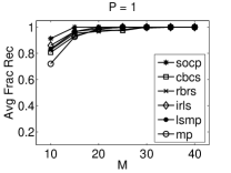
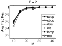
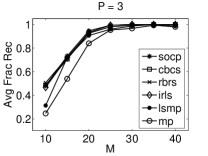
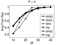
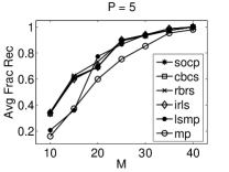
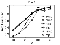
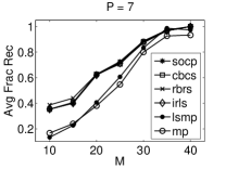
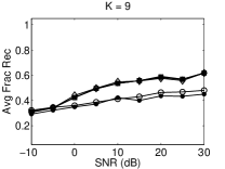
Each subplot of Fig. 1 depicts the average fraction of recovered sparsity profile elements versus the number of knowns, , for a fixed value of , revealing how performance varies as the matrices go from being underdetermined to overdetermined.
 |
 |
 |
 |
 |
 |
 |
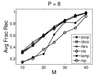 |
Recovery Trends. As the number of knowns increases, recovery rates improve substantially, which is sensible. For large and small , the six algorithms behave similarly, consistently achieving nearly 100% recovery. For large and moderate , however, sparsity profile recovery rates are dismal—as increases, the underlying simultaneous sparsity of the s is not enough to combat the increasing number of unknowns, . As is decreased and especially when is increased, the performance of the greedy techniques falls off relative to that of IRLS, RBRS, CBCS, and SOCP, showing that the convex relaxation approach itself is a sensible way to approximately solve the formal NP-Hard combinatorial MSSO simultaneous sparsity problem. Furthermore, the behavior of the convex algorithms relative to the greedy ones coincides with the studies of greedy vs. convex programming sparse approximation methods in single-vector [4, 6] and SSMO contexts [7]. Essentially, in contrast with convex programming techniques, the greedy algorithms only look ahead by one term, cannot backtrack on sparsity profile element choices, and do not consider updating multiple rows of unknowns of the matrix at the same time. LSMP tends to perform slightly better than MP because it solves a least squares minimization and explicitly considers earlier chosen rows whenever it seeks to choose another row of .
Convergence. Across most trials, IRLS, RBRS, CBCS, and SOCP converge rapidly and do not exceed the maximum limit of 500 outer iterations. The exception is CBCS when is small and : here, the objective function frequently fails to decrease by less than the specified .
Runtimes. For several fixed pairs, Table 1 lists the average runtimes of each algorithm across the 50 trials associated with each pair.555In the interest of space we do not list average runtimes for all fifty-six pairs. For IRLS, RBRS, CBCS, and SOCP, runtimes are also averaged over the many runs. Among the convex minimization methods, SOCP seems superior given its fast runtimes in three out of four cases. Peak memory usage is not tracked here because it is difficult to do so when using MATLAB for such small problems; it will be tracked during the third experiment where the system matrices are vastly larger and differences in memory usage across the six algorithms are readily apparent.
| Algorithm | (10,8) | (20,1) | (30,5) | (40,8) |
|---|---|---|---|---|
| MP | 5.4 | 1.8 | 2.6 | 4.0 |
| LSMP | 11.4 | 5.6 | 15.6 | 27.6 |
| IRLS | 92.6 | 10.1 | 73.2 | 175.0 |
| RBRS | 635.7 | 36.0 | 236.8 | 401.6 |
| CBCS | 609.8 | 7.1 | 191.4 | 396.3 |
| SOCP | 44.3 | 37.0 | 64.3 | 106.5 |
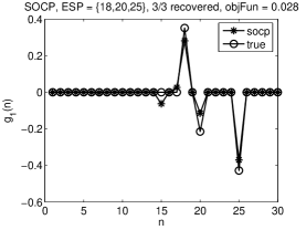
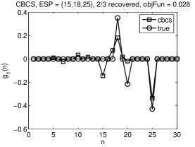
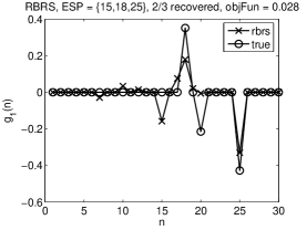
Closer Look: Solution Vectors. We now observe how the algorithms that seek to minimize the convex objective behave during the 43rd trial when , , , and , corresponding to the base case problem of estimating one sparse real-valued vector, . Fig. 2 illustrates estimates obtained by SOCP, CBCS, RBRS, and IRLS when ; for each algorithm, a subplot shows elements of both the estimated and actual , and lists the estimated sparsity profile (ESP), number of profile terms recovered, and value of the objective function given in (9, 13). Although RBRS, CBCS, and SOCP yield slightly different solutions (among which SOCP yields the best profile estimate), they all yield an objective function equal to . Convex combinations of the three solutions continue to yield the same value, suggesting that the three algorithms have found solutions among a convex set that is the global solution to the objective posed in (9, 13). Given the fact that in this case SOCP outperforms RBRS and CBCS, we see that even the globally optimal solution to the relaxed convex objective does not necessarily optimally solve the true -sparse profile recovery problem. In contrast to the other methods, IRLS yields a slightly higher objective function value, 0.030, and its solution vector is not part of the convex set—it does however correctly determine 2 of the 3 terms of the true sparsity profile.
 |
 |
 |
 |
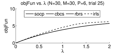
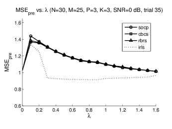
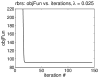
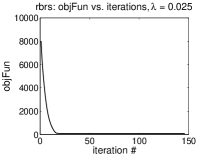
Closer Look: Objective Function Behavior. Concluding the experiment, Fig. 3 plots the objective vs. for the 25th trial when and , studying how the objective (9, 13) varies with when applying SOCP, CBCS, RBRS, and IRLS. For all seventy values of , SOCP, CBCS, and RBRS generate solutions that yield the same objective function value. For , IRLS attains the same objective function value as the other methods, but as increases, IRLS is unable to minimize the objective function as well as SOCP, RBRS, and CBCS. The behavior in Fig. 3 occurs consistently across the fifty trials of the other pairs.
5.2 Sparsity Profile Estimation in the Presence of Noise
5.2.1 Overview
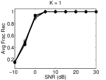
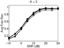
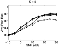
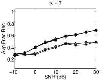
We now evaluate how well the algorithms of Sec. 4 estimate sparsity profiles when the underlying s are each strictly and simultaneously -sparse and the observation of (7) is corrupted by additive white Gaussian noise. The signal-to-noise ratio (SNR) and are varied across sets of Monte Carlo trials in order to gauge algorithm performance across many scenarios. For a given trial with a fixed SNR level in units of decibels (dB), the elements of the true observation vector, , are corrupted with independent and identically distributed (i.i.d.) zero-mean Gaussian noise with variance , related to the SNR as follows:
| (43) |
This noise measure is analogous to that of [7].
5.2.2 Details
We fix , , and , and consider and . For each fixed pair, we generate 100 noisy observations and apply the algorithms as follows:
-
Generate the sparsity profile, s, s, s, and s as in Sec. 5.1.2. The s are simultaneously -sparse and all terms are real-valued.
-
Compute .
-
Construct where and is given by (43).
-
Apply the algorithms by providing them with and the system matrices:
-
MP, LSMP: iterate until elements are chosen or the residual approximation is . If less than terms are chosen, this hurts the recovery score.
-
IRLS, RBRS, CBCS, SOCP: using a pre-determined fixed (see below), apply each algorithm to obtain estimates of the unknown vectors and sparsity profiles.
-
After performing the above steps, we average the results of the 100 trials associated with each fixed triplet to yield the average fraction of sparsity profile elements that each algorithm recovers.
Control Parameter Selection. The mentioned in the list above is determined as follows: before running the overall experiment, we generate three noisy observations for each pair. We then apply IRLS, RBRS, CBCS, and SOCP, tuning the control parameter by hand until finding a single value that produces reasonable solutions. All algorithms then use this hand-tuned, fixed and are applied to the other 100 noisy observations associated with the pair under consideration. Thus, in distinct contrast to the noiseless experiment, we no longer assume an ideal is known for each denoising trial.
5.2.3 Results
Each subplot of Fig. 4 depicts the average fraction of recovered sparsity profile elements versus SNR for a fixed , revealing how well the six algorithms are able to recover the elements of the sparsity profile amidst noise in the observation. Each data point is the average fraction recovered across 100 trials.
Recovery Trends. When , we see from the upper-left subplot of Fig. 4 that all algorithms have essentially equal performance for each SNR. Recovery rates improve substantially with increasing SNR, which is sensible. For each algorithm, we see across the subplots that performance generally decreases with increasing ; in other words, estimating a large number of sparsity profile terms is more difficult than estimating a small number of terms. This trend is evident even at high SNRs. For example, when SNR is 30 dB and , SOCP is only able to recover of sparsity profile terms. When , the recovery rate falls to . For low SNRs, e.g., -5 dB, all algorithms tend to perform similarly, but the greedy algorithms perform increasingly worse than the others as goes from moderate-to-large and SNR surpasses zero dB. In general, MP performs worse than LSMP, and LSMP in turn performs worse than IRLS, SOCP, RBRS, and CBCS, while the latter four methods exhibit essentially the same performance across all SNRs and s. For , MP’s performance falls off relative to IRLS, SOCP, RBRS, and CBCS, but LSMP’s does not. As transitions from 3 to 5, however, LSMP performs as badly as MP at low SNRs, but its performance picks up as SNR increases. As continues to increase beyond 5, LSMP’s performance is unable to surpass that of MP, even when SNR is large. Overall, Fig. 4 shows that convex programming algorithms are superior to greedy methods when estimating sparsity profiles in noisy situations; this coincides with data collected in the noiseless experiment in Sec. 5.1, as well as the empirical findings of [6, 7].
 |
 |
 |
 |
 |
Convergence. For many denoising trials, CBCS typically requires more iterations than the other techniques in order to converge. At times, it fails to converge to within the specified , similarly to how it behaves during the noiseless experiment of Sec. 5.1.
Runtimes. Across all denoising trials, MP, LSMP, IRLS, RBRS, CBCS, SOCP have average runtimes of 3.1, 25.1, 57.2, 247.0, 148.5, and 49.2 milliseconds. It seems SOCP is best for denoising given that it is the fastest algorithm among the four methods that outperforms the greedy ones. IRLS is nearly as fast as SOCP and thus is a close second choice for sparsity profile estimation.
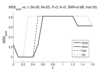
Closer Look: Mean Square Errors of Convex Minimization Methods Before and After Estimating the Sparsity Profile and Retuning the Solution. Now let us consider the th trial of the pair. We do away with the fixed assumption and now assume we care (to some extent) not only about estimating the sparsity profile, but the true solution as well. To proxy for this, we study how the mean square errors (MSEs) of solutions generated by IRLS, SOCP, RBRS, and CBCS behave across before and after identifying the sparsity profile and retuning the solution. Figure 5 depicts the results of this investigation.
Running each algorithm for a particular yields a solution . The left subplot simply illustrates the MSEs of the s with respect to the true solution. Among SOCP, RBRS, CBCS, and IRLS, only the last is able to determine solutions with MSEs less than unity (consider the IRLS error curve for ).
Consider now retuning each of the s as follows: unstack each into for and then remember the vectors whose energies are largest, yielding an estimate of the -element sparsity profile. Let these estimated indices be . Now, generate a retuned solution by using the matrices associated with the estimated sparsity profile and solving for . This latter vector consists of elements and by unstacking it we obtain a retuned estimate of the s, e.g., equals the first elements of , and so forth, while the other s for are now simply all-zeros vectors. Reshuffling the retuned s yields s that are strictly and simultaneously sparse whose weightings yield the best match to the noisy observation in the sense. Unlike the original solution estimate, which is not necessarily simultaneously -sparse, here we have enforced true simultaneous -sparsity. We may or may not have improved the MSE with respect to the true solution: for example, if we have grossly miscalculated the sparsity profile, the MSE of the retuned solution is likely to increase substantially, but if we have estimated the true sparsity profile exactly, then the retuned solution will likely be quite close (in the sense) to the true solution, and MSE will thus decrease.
The MSEs of these retuned solutions with respect to the true are plotted in the right subplot of Fig. 5. For all algorithms and s, MSE has increased relative to the left subplot, which means that in every case our estimate of the true underlying solution has worsened. This occurs because across all algorithms and s in Fig. 5, the true -term sparsity profile is incorrectly estimated and thus the retuning step makes the estimated solution worse. The lesson here is that if one is interested in minimizing MSE in low-to-moderate SNR regimes it may be best to simply keep the original estimate of the solution rather than detect the sparsity profile and retune the result. If one is not certain that the sparsity profile estimate is accurate, retuning is likely to increase MSE by fitting the estimated solution weights to an incorrect set of generating matrices. On the other hand, if one is confident that the entire sparsity profile will be correctly identified with sufficiently high probability, retuning will be beneficial; see [18, 24, 20] for related ideas.
 |
 |
5.3 MRI RF Excitation Pulse Design
5.3.1 Overview
For the final experiment we study how well the six algorithms design MRI RF excitation pulses. In the interest of space and because the conversion of the physical problem into an MSSO format involves MRI physics and requires significant background, we only briefly outline how the system matrices arise and why simultaneously sparse solutions are necessary. A complete formulation of the problem for engineers and mathematicians is given in [51]; MRI pulse designers may refer to [53].
5.3.2 Formulation
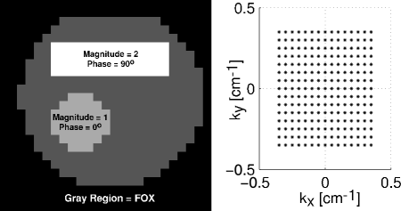
For the purposes of this paper, the design of an MRI RF excitation pulse reduces to the following problem: assume we are given points in the 2-D spatial domain, , along with points in a 2-D “Fourier-like” domain, . Each equals , a point in space, while each equals , a point in the Fourier-like domain, referred to as “-space”. The s and s are in units of centimeters (cm) and inverse centimeters (), respectively. The s are Nyquist-spaced relative to the sampling of the s and may be visualized as a 2-D grid located at low and frequencies (where “” denotes the frequency domain axis that corresponds to the spatial axis). Under reasonable assumptions, energy placed at one or more points in -space produces a pattern in the spatial domain; this pattern is related to the -space energy via a “Fourier-like” transform [39]. Assume we place an arbitrary complex weight (i.e., both a magnitude and phase) at each of the locations in -space. Let us represent these weights using a vector . In an ideal (i.e., physically-unrealizable) setting, the following holds:
| (44) |
where is a known dense Fourier matrix666Formally, , where and is a known lumped gain constant. and the th element of is the image that arises at , denoted , due to the energy deposition along the points on the -space grid as described by the weights in the vector.
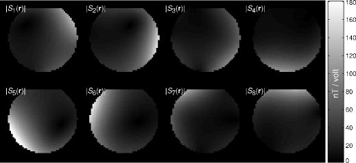
The goal now is to form a desired (possibly complex-valued) spatial-domain image at the given set of spatial domain coordinates (the s) by placing energy at some of the given locations while obeying a special constraint on how the energy is deposited. To produce the spatial-domain image, we will use a “-channel MRI parallel excitation system” [29, 41]—each of the system’s channels is able to deposit energy of varying magnitudes and phases at the -space locations and is able to influence the resulting spatial-domain pattern to some extent. Each channel has a known “profile” across space, , that describes how the channel is able to influence the magnitude and phase of the resulting image at different spatial locations. For example, if , then the 3rd channel is unable to influence the image that arises at location , regardless of how much energy it deposits along . The special constraint mentioned above is as follows: the system’s channels may only visit a small number of points in -space—they may only deposit energy at locations.
We now finalize the formulation of problem: first, we construct diagonal matrices such that . Now we assume that each channel deposits arbitrary energies at each of the points in -space and describe the weighting of the -space grid by the th channel with the vector . Based on the physics of the -channel parallel excitation system, the overall image that forms is the superposition of the profile-scaled subimages produced by each channel:
| (45) |
where . Essentially, (45) is the real-world version of (44) for -channel systems with profiles that are not constant across .
Recalling that our overall goal is to deposit energy in -space to produce the image , and given the special constraint that we may only deposit energy among a small subset of the points in -space, we arrive at the following problem:
| (46) |
where and is given by (45). That is, we seek out locations in -space at which to deposit energy to produce an image that is close in the sense to the desired image . Strictly and simultaneously -sparse s are the only valid solutions to the problem.
One sees that (46) is precisely the MSSO system given in (8) and thus the algorithms posed in Sec. 4 are applicable to the pulse design problem. In order to apply the convex minimization techniques (IRLS, SOCP, RBRS, and CBCS) to this problem, the only additional step needed is to retune any given solution estimate into a strictly and simultaneously -sparse set of vectors; this retuning step is computationally tractable and was described in Sec. 5.2.3’s “Closer Look” subsection.
Aside. An alternative approach to decide where to place energy at locations in -space is to compute the Fourier transform of and decide to place energy at frequencies where the Fourier coefficients are largest in magnitude [50]. This method does yield valid -sparse energy placement patterns, but empirically it is always outperformed by the convex minimization approaches [52, 51, 53] so we do not delve into the Fourier-based method in this paper.
5.3.3 Experimental Setup
Using an eight-channel system (i.e., ) whose profile magnitudes (the s) are depicted in Fig. 6, we will design pulses to produce the desired complex-valued image shown in the left subplot of Fig. 7. We sample the spatial domain at locations within the region where at least one of the profiles in Fig. 6 is active—this region of interest is referred to as the field of excitation (FOX) in MRI literature.777Sampling points outside of the FOX where no profile has influence is unnecessary because an image can never be formed at these points no matter how much energy any given channel places throughout -space. The spatial samples are spaced by 0.8 cm along each axis and the FOX has a diameter of roughly 20 cm. Given our choice of , we sample the s and and construct the s and . Next, we define a grid of points in -space that is in size and extends outward from the -space origin. The points are spaced by along each -space axis and the overall grid is shown in the right subplot of Fig. 7. Finally, because we know the 356 s and 225 s, we construct the matrix in (44, 45) along with the s in (45). We now have all the data we need to apply the algorithms and determine simultaneously -sparse s that (approximately) solve (46).
 |
 |
We apply the algorithms and evaluate designs where the use of candidate points in -space is permitted (in practical MRI scenarios, up to 30 is permissible). Typically, the smallest possible that produces a version of to within some -fidelity is the design that the MRI pulse designer will use on a real system.
To obtain simultaneously -sparse solutions with MP and LSMP, we set , run each algorithm once, remember the ordered list of chosen indices, and back out every solution for through via the retuning technique of Sec. 5.2.3.
For each convex minimization method (IRLS, SOCP, RBRS, and CBCS), we apply the following procedure: first, we run the algorithm for 14 values of , storing each resulting solution, . Then for fixed , to determine a simultaneously -sparse deposition of energy on the -space grid, we apply the retuning process of Sec. 5.2.3 to each of the 14 solutions, obtaining 14 strictly simultaneously -sparse retuned sets of solution vectors, . The one solution among the 14 that best minimizes the error between the desired and resulting images, , is chosen as the solution for the under consideration. Essentially, we again assume we know a good value for when applying each of the convex minimization methods. To attempt to avoid convergence problems, RBRS and CBCS are permitted 5,000 and 10,000 maximum outer iterations, respectively (see below).
5.3.4 Results
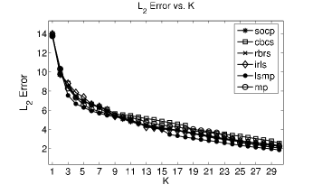
Image Error vs. Number of Energy Depositions in -Space. Figure 8’s left subplot shows the error versus curves for each algorithm. As is increased, each method produces images with lower error, which is sensible: depositing energy at more locations in -space gives each technique more degrees of freedom with which to form the image. In contrast to the sparsity profile estimation experiments in Sec. 5.1 and Sec. 5.2, however, here LSMP is the best algorithm: for each fixed considered in Fig. 8, the LSMP technique yields a simultaneously -sparse energy deposition that produces a higher-fidelity image than all other techniques. For example, when LSMP yields a solution that leads to an image with error of 3.3. In order to produce an image with equal or better fidelity, IRLS, RBRS, and SOCP need to deposit energy at points in -space, and thus produce less useful designs from an MRI perspective. CBCS fares the worst, needing to deposit energy at grid points in order to compete with the fidelity of LSMP’s image.
 |
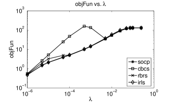 |
Closer Look: Objective Function vs. . The right subplot of Fig 8 shows how well the four convex minimization algorithms minimize the objective function (9, 13) before retuning any solutions and enforcing strict simultaneous -sparsity. For each fixed , SOCP and IRLS find solutions that yield the same objective function value. RBRS’s solutions generally yield objective function values equal to those of SOCP and IRLS, but at times lead to higher values: in these cases RBRS almost converges but does not do so completely. Finally, for most s CBCS’s solutions yield extremely large objective function values; in these cases CBCS completely fails to converge.
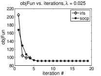
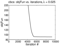
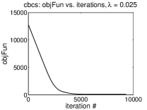
Closer Look: Objective Function Convergence for . The right subplot of Fig 8 shows that for , IRLS, SOCP, RBRS, and CBCS generate solutions that yield the same objective function value, suggesting that each method succeeds at minimizing the objective function. Figure 9 illustrates how the algorithms converge in this specific case: each subplot tracks the value of an algorithm’s objective function as it iterates. Subplots along the top row all have the same axis, giving a close look at how the algorithms behave. The two subplots along the bottom row “zoom out” along the axis to show RBRS’s and CBCS’s total behavior. IRLS and SOCP converge rapidly, within 4 and 19 iterations, respectively. RBRS requires roughly 150 outer iterations, while CBCS requires nearly 10,000.
 |
 |
 |
 |
 |
Runtimes and Peak Memory Usage. Setting , we run MP and LSMP and record the runtime of each. Across the 14 s, IRLS, RBRS, CBCS, and SOCP’s runtimes are recorded and averaged. The peak memory usage of each algorithm is also noted; these statistics are presented in Table 2. In distinct contrast to the smaller-variable-size experiments in Sec. 5.1 and Sec. 5.2 where all four convex minimization methods have relatively short runtimes (under one second), here RBRS and CBCS are much slower, leaving IRLS and SOCP as the only feasible techniques among the four. Furthermore, while LSMP does indeed outperform IRLS and SOCP on an error basis (as shown in Fig. 8), the runtime statistics here show that LSMP requires order-of-magnitude greater runtime to solve the problem—therefore, in some real-life scenarios where designing pulses in less than 5 minutes is a necessity, IRLS and SOCP are superior. Finally, in contrast to Sec. 5.1’s runtimes given in Table 1, here IRLS is 1.9 times faster than SOCP and uses 1.4 times less peak memory, making it the superior technique for MRI pulse design since IRLS’s error performance and ability to minimize the objective function (9, 13) essentially equal that of SOCP.
| Algorithm | Runtime | Peak Memory Usage (MB) |
|---|---|---|
| MP | 11 sec | 704 |
| LSMP | 46 min | 304 |
| IRLS | 50 sec | 320 |
| RBRS | 87 min | 320 |
| CBCS | 3.3 hr | 320 |
| SOCP | 96 sec | 432 |
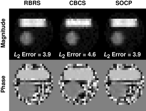
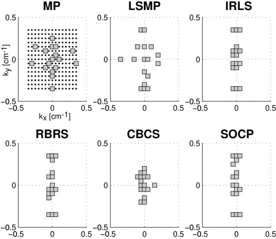
Closer Look: Images and Chosen -Space Locations for . To conclude the experiment, we fix and observe the images produced by the algorithms along with the points at which each algorithm chooses to deposit energy along the grid of candidate points in -space. Figure 10 illustrates the images (in both magnitude and phase) that arise due to each algorithm’s simultaneously 17-sparse set of solution vectors,888Each image is generated by taking the corresponding solution , computing in (45), unstacking the elements of into , and then displaying the magnitude and phase of . while Fig. 11 depicts the placement pattern chosen by each method. From Fig. 10, we see that each algorithm forms a high-fidelity version of the desired image given in the left subplot of Fig. 7, but among the images, LSMP’s most accurately represents (e.g., consider the sharp edges of the LSMP image’s rectangular box). MP’s and CBCS’s images are noticeably fuzzy relative to the others. The placements in Fig. 11 give insight into these performance differences. Here, LSMP places energy at several higher frequencies along the and axes, which ensures the resulting rectangle is narrow with sharp edges along the spatial and axes. In contrast, CBCS fails to place energy at moderate-to-high -space frequencies and thus cannot produce a rectangle with desirable sharp edges, while MP branches out to some extent but fails to utilize high frequencies. IRLS, RBRS, and SOCP branch out to higher frequencies but not to high frequencies, and thus their associated rectangles in Fig. 10 are sharp along the axis but exhibit less distinct transitions (more fuzziness) along the spatial axis. In general, each algorithm has determined 17 locations at which to place energy that yield a fairly good image and each has avoided the computationally impossible scenario of searching over all -choose- (225-choose-17) possible placements.
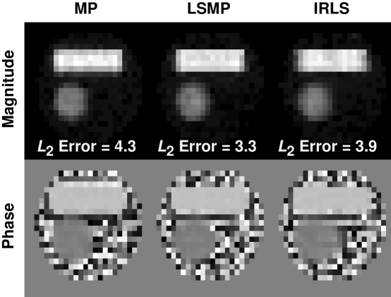 |
 |
 |
6 Discussion
6.1 MRI Pulse Design vs. Denoising and Source Localization
The MRI pulse design problem in Sec. 5.3 differs
substantially from the source localization problem in
Sec. 5.1, the denoising experiment in
Sec. 5.2, and other routine applications of sparse
approximation (e.g. [11, 4, 20, 16, 6, 7, 33]). It differs not only in purpose but in
numerical properties, the latter of which are summarized in
Table 3. While this list will not always hold true
on an application-by-application basis, it does highlight general
differences between the two problem classes.
| MRI Pulse Design | Denoising and Source Localization |
|---|---|
| s overdetermined | s underdetermined |
| No concept of noise: given is | Noisy: given is not |
| Sweep over useful | Ideal unknown |
| Metric: | Metrics: , and/or |
| fraction of rec. sparsity profile terms |
6.2 Merits of Row-by-Row and Column-by-Column Shrinkage
Even though LSMP, IRLS, and SOCP tend to exhibit superior performance across different experiments in this manuscript, RBRS and CBCS are worthwhile because unlike the former methods that update all unknowns concurrently, the shrinkage techniques update only a subset of the total variables during each iteration.
For example, RBRS as given in Algorithm 5 updates only unknowns at once, while CBCS as given in Algorithm 6 updates but a single scalar at a time. RBRS and CBCS are thus applicable in scenarios where and are exceedingly large and tuning all parameters during each iteration is not possible. If storing and handling or matrices exceeds a system’s available memory and causes disk thrashing, RBRS and CBCS, though they require far more iterations, might still be better options than LSMP, IRLS, and SOCP in terms of runtime.
6.3 Future Work
6.3.1 Efficient Automated Control Parameter Selection
6.3.2 Runtime, Memory, and Complexity Reduction
As noted in Sec. 4, LSMP’s computation and runtime could be improved upon by extending the projection based recursive updating schemes of [6, 7] to MSSO LSMP. In regards to the MRI design problem, runtime for any method might be reduced via a multi-resolution approach (as in [33]) by first running the algorithm with a coarse -space frequency grid, noting which energy deposition locations are revealed, and then running the algorithm with a grid that is finely sampled around the locations suggested by the coarse result. This is faster than providing the algorithm a large, finely-sampled grid and attempting to solve the sparse energy deposition task in one step. An initial investigation has shown that reducing the maximum frequency extent of the -space grid (and thus the number of grid points, ) may also reduce runtime without significantly impacting image fidelity [53].
6.3.3 Shrinkage Algorithm Convergence Improvements
When solving the MRI pulse design problem, both RBRS and CBCS required excessive iterations and hence exhibited lengthy runtimes. The latter was especially problematic as illustrated in Fig. 9. To mitigate these problems, one may consider extending parallel coordinate descent (PCD) shrinkage techniques used for single-system single-output sparse approximation (as in [15, 16]). Sequential subspace optimization (SESOP) [17] might also be employed to reduce runtime. Combining PCD with SESOP and adding a line search after each iteration would yield sophisticated versions of RBRS and CBCS.
6.3.4 Multiple-System Multiple-Output (MSMO) Simultaneous Sparse Approximation
In the future it may be useful to consider a combined problem where there are multiple observations as well as multiple system matrices. That is, assume we have a series of observations, , each of which arises due to a set of simultaneously -sparse unknown vectors 999The -term simultaneous sparsity profile of each set of s may or may not change with . passing through a set of system matrices and then undergoing linear combination, as follows:
| (47) |
If is constant for all observations then the problem reduces to
| (48) |
and we may stack the matrices and terms as follows:
| (49) |
Having posed (47, 48, 49), one may formulate optimization problems similar to (5, 9) to determine simultaneously sparse s that solve (49). Algorithms to solve such problems may arise by combining the concepts of SSMO algorithms [7, 33, 49, 47] with those of the MSSO algorithms posed earlier.
7 Conclusion
We defined the linear inverse multiple-system, single-output (MSSO) simultaneous sparsity problem where simultaneously sparse sets of unknown vectors are required as the solution. This problem differed from prior problems involving multiple unknown vectors because in this case, each unknown vector was passed through a different system matrix and the outputs of the various matrices underwent linear combination, yielding only one observation vector.
To solve the proposed MSSO problem, we formulated three greedy techniques, matching pursuit, orthogonal matching pursuit, and least squares matching pursuit, along with algorithms based on iteratively reweighted least squares, iterative shrinkage, and second-order cone programming methodologies. The MSSO algorithms were evaluated across noiseless and noisy sparsity profile estimation experiments as well as a magnetic resonance imaging pulse design experiment; for sparsity profile recovery, algorithms that minimized the relaxed convex objective function outperformed the greedy methods, whereas in the noiseless magnetic resonance imagine pulse design experiment, greedy LSMP exhibited superior performance.
Finally, when deriving CBCS for complex-valued data, we proved that seeking a single sparse complex-valued vector is equivalent to seeking two simultaneously sparse real-valued vectors—we mapped single-vector sparse approximation of a complex vector to the MSSO problem, increasing the applicability of algorithms that solve the latter.
Overall, while improvements upon these seven algorithms (and new algorithms altogether) surely do exist, this manuscript has laid the groundwork of the MSSO problem and conducted an initial exploration of algorithms with which to solve it.
Acknowledgments
The authors thank D. M. Malioutov for assistance with the derivation step that permitted the transition from (41) to (42) in Sec. 4.7, as well as K. Setsompop, B. A. Gagoski, V. Alagappan, and L. L. Wald for collecting the experimental coil profile data in Fig. 6.
The authors gratefully acknowledge the following sponsors and associated grants: National Institute of Health 1P41RR14075, 1R01EB000790, 1R01EB006847, and 1R01EB007942; NSF CAREER Award CCF-643836; United States Department of Defense National Defense Science and Engineering Graduate Fellowship F49620-02-C-0041; the MIND Institute; the A. A. Martinos Center for Biomedical Imaging; and R. J. Shillman’s Career Development Award.
References
- [1] A. Bjorck and T. Elfving, Accelerated projection methods for computing pseudoinverse solutions of systems of linear equations, Tech. Report LiTH-MAT-R-1978-5, Department of Mathematics, Linkoping Univ., 1978.
- [2] S. Boyd and L. Vandenberghe, Convex Optimization, Cambridge Univ. Press, Mar. 2004.
- [3] S. Chen and J. Wigger, Fast orthogonal least squares algorithm for efficient subset model selection, IEEE Trans. Signal Process., 43 (1995), pp. 1713–1715.
- [4] S. S. Chen, D. L. Donoho, and M. A. Saunders, Atomic decomposition by basis pursuit, SIAM J. Sci. Comput., 20 (1998), pp. 33–61.
- [5] P. L. Combettes and J. C. Pesquet, Proximal Thresholding Algorithm for Minimization over Orthogonal Bases, SIAM J. Optimiz., 18 (2007), pp. 1351–1376.
- [6] S. F. Cotter, J. Adler, B. D. Rao, and K. Kreutz-Delgado, Forward sequential algorithms for best basis selection, in Proc. Inst Elect Eng Vision, Image, Signal Process., vol. 146, Oct. 1999, pp. 235–244.
- [7] S. F. Cotter, B. D. Rao, K. Engan, and K. Kreutz-Delgado, Sparse solutions to linear inverse problems with multiple measurement vectors, IEEE Trans. Signal Process., 53 (2005), pp. 2477–2488.
- [8] I. Daubechies, M. Defrise, and C. De Mol, An iterative thresholding algorithm for linear inverse problems with a sparsity constraint, Comm. Pure Appl. Math, 57 (2004), pp. 1413–1457.
- [9] G. Davis, Adaptive Nonlinear Approximations, PhD thesis, New York Univ., 1994.
- [10] G. Davis, S. Mallat, and M. Avellaneda, Greedy adaptive approximation, Constr. Approx., 13 (1997), pp. 57–98.
- [11] D. L. Donoho, De-noising by soft-thresholding, IEEE Trans. Inform. Theory, 41 (1995), pp. 613–627.
- [12] , For most large underdetermined systems of equations, the minimal -norm near-solution approximates the sparsest near solution, Commun. Pure Appl. Math., 59 (2006), pp. 907–934.
- [13] D. L. Donoho, M. Elad, and V. N. Temlyakov, Stable recovery of sparse overcomplete representations in the presence of noise, IEEE Trans. Inform. Theory, 52 (2006), pp. 6–18.
- [14] D. L. Donoho and I. M. Johnstone, Ideal spatial adaptation by wavelet shrinkage, Biometrika, 81 (1994), pp. 425–455.
- [15] M. Elad, Why simple shrinkage is still relevant for redundant representations?, IEEE Trans. Inform. Theory, 52 (2006), pp. 5559–5569.
- [16] M. Elad, B. Matalon, and M. Zibulevsky, Image denoising with shrinkage and redundant representations, in Proc. IEEE CVPR, vol. 2, 2006, pp. 1924–1931.
- [17] , Coordinate and subspace optimization methods for linear least squares with non-quadratic regularization, Appl. Comput. Harm. Anal., 23 (2007), pp. 346–367.
- [18] M. Elad and I. Yavheh, A weighted average of sparse representations is better than the sparsest one alone, IEEE Trans. Inform. Theory, Submitted (2008).
- [19] M. A. T. Figueiredo, R. D. Nowak, and S. J. Wright, Gradient projection for sparse reconstruction: Application to compressed sensing and other inverse problems, IEEE J. Sel. Topics in Signal Process., 1 (2007), pp. 586–597.
- [20] A. K. Fletcher, S. Rangan, V. K. Goyal, and K. Ramchandran, Denoising by sparse approximation: Error bounds based on rate–distortion theory, EURASIP J. Applied Signal Process., 2006 (2006), pp. 1–19.
- [21] G. H. Golub and W. Kahan, Calculating the singular values and pseudoinverse of a matrix, SIAM J. Num. Anal., 2 (1965), pp. 205–224.
- [22] G. H. Golub and C. F. Van Loan, Matrix Computations, Johns Hopkins Univ. Press, 1983.
- [23] I. F. Gorodnitsky and B. D. Rao, Sparse signal reconstruction from limited data using FOCUSS: A recursive weighted norm minimization algorithm, IEEE Trans. Signal Process., 45 (1997), pp. 600–616.
- [24] V. K. Goyal, A. K. Fletcher, and S. Rangan, Compressive sampling and lossy compression, IEEE Signal Process. Mag., 25 (2008), pp. 48–56.
- [25] P. C. Hansen, Regularization tools: A Matlab package for analysis and solution of discrete ill-posed problems, Num. Alg., 6 (1994), pp. 1–35.
- [26] D. H. Johnson and D. E. Dudgeon, Array Signal Processing–Concepts and Techniques, Prentice Hall, 1993.
- [27] I. M. Johnstone, On minimax estimation of a sparse normal mean vector, Ann. Stat., 22 (1994), pp. 271–289.
- [28] L. A. Karlovitz, Construction of nearest points in the , even and norms, J. Approx. Theory, 3 (1970), pp. 123–127.
- [29] U. Katscher, P. Bornert, C. Leussler, and J. S. van den Brink, Transmit SENSE, Magn. Reson. Med., 49 (2003), pp. 144–150.
- [30] H. Krim and M. Viberg, Two decades of array signal processing research. the parametric approach., IEEE Sig Process. Mag, 13 (1996), pp. 67–94.
- [31] C. Lanczos, An iteration method for the solution of the eigenvalue problem of linear differential and integral operators, J. Research of the National Bureau of Standards, 45 (1950), pp. 255–282.
- [32] D. M. Malioutov, A sparse signal reconstruction perspective for source localization with sensor arrays, master’s thesis, Massachusetts Institute of Technology, 2003.
- [33] D. M. Malioutov, M. Çetin, and A. S. Willsky, A sparse signal reconstruction perspective for source localization with sensor arrays, IEEE Trans. Signal Process., 53 (2005), pp. 3010–3022.
- [34] S. G. Mallat and Z. Zhang, Matching pursuits with time-frequency dictionaries, IEEE Trans. Signal Process., 41 (1993), pp. 3397–3415.
- [35] B. K. Natarajan, Sparse approximate solutions to linear systems, SIAM J. Sci. Comput., 24 (1995), pp. 227–234.
- [36] A. Nemirovski and A. Ben-Tal, Lectures on Modern Convex Optimization: Analysis, Algorithms, and Engineering Applications, SIAM, Philadelphia, PA, USA, 2001.
- [37] C. C. Paige and M. A. Saunders, Algorithm 583; LSQR: Sparse linear equations and least-squares problems, ACM Trans. Mathemat. Softw., 8 (1982), pp. 195–209.
- [38] , LSQR: An algorithm for sparse linear equations and sparse least squares, ACM Trans. Mathemat. Softw., 8 (1982), pp. 43–71.
- [39] J. M. Pauly, D. Nishimura, and A. Macovski, A -space analysis of small-tip-angle excitation, J. Magn. Reson., 81 (1989), pp. 43–56.
- [40] B. D. Rao, Signal processing with the sparseness constraint, in Proc. ICASSP, vol. 3, Seattle, WA, May 1998, pp. 1861–1864.
- [41] K. Setsompop, L. L. Wald, V. Alagappan, B. A. Gagoski, F. Hebrank, U. Fontius, F. Schmitt, and E. Adalsteinsson, Parallel RF transmission with 8 channels at 3 Tesla, Magn. Reson. Med., 56 (2006), pp. 1163–1171.
- [42] J. Sturm, Using SeDuMi 1.02, a MATLAB toolbox for optimization over symmetric cones, Optimiz. Meth. Softw., 11–12 (1999), pp. 625–653. Special issue on Interior Point Methods.
- [43] R. Tibshirani, Regression shrinkage and selection via the LASSO, J. Royal Stat. Soc., Series B, 58 (1996), pp. 267–288.
- [44] A. N. Tikhonov, Solution of incorrectly formulated problems and the regularization method, Doklady Akademii Nauk SSSR, 151 (1963), pp. 501–504.
- [45] A. N. Tikhonov and V. A. Arsenin, Solution of Ill-posed Problems, Winston & Sons, Washington, DC, USA, 1977.
- [46] K. C. Toh, M. J. Todd, and R. H. Tutuncu, SDPT3 - a matlab software package for semidefinite programming, Optimiz. Meth. Softw., 11 (1999), pp. 545–581.
- [47] J. A. Tropp, Algorithms for simultaneous sparse approximation: part II: Convex relaxation, Signal Process., 86 (2006), pp. 589–602.
- [48] , Just relax: Convex programming methods for identifying sparse signals in noise, IEEE Trans. Inform. Theory, 52 (2006), pp. 1030–1051.
- [49] J. A. Tropp, A. C. Gilbert, and M. J. Strauss, Algorithms for simultaneous sparse approximation: part I: Greedy pursuit, Signal Process., 86 (2006), pp. 572–588.
- [50] C. Y. Yip, J. A. Fessler, and D. C. Noll, Advanced 3-D tailored RF pulse for signal recovery in T-weighted functional magnetic resonance imaging, Magn. Reson. Med., 56 (2006), pp. 1050–1059.
- [51] A. C. Zelinski, V. K. Goyal, E. Adalsteinsson, and L. L. Wald, Sparsity in MRI RF excitation pulse design, in Proc. Conf. Inform. Sci. Syst. (Princeton, NJ), Mar. 2008, pp. 252–257.
- [52] A. C. Zelinski, K. Setsompop, V. K. Goyal, V. Alagappan, U. Fontius, F. Schmitt, L. L. Wald, and E. Adalsteinsson, Designing fast 3-D RF excitations by optimizing the number, placement, and weighting of spokes in -space via a sparsity-enforcement algorithm, in Proc. Int. Soc. for Magnetic Resonance in Medicine (ISMRM), Berlin, Germany, 2007, p. 1691.
- [53] A. C. Zelinski, L. L. Wald, K. Setsompop, V. K. Goyal, and E. Adalsteinsson, Sparsity-enforced slice-selective MRI RF excitation pulse design, IEEE Trans. Med. Imaging, 27 (2008), pp. 1213–1229.