Next-to-Leading Order QCD Predictions for $W$ + 3-Jet Distributions at Hadron Colliders

Abstract

We present next-to-leading order QCD predictions for a variety of distributions in $W\,\!+\,3$-jet production at both the Tevatron and the Large Hadron Collider. We include all subprocesses and incorporate the decay of the $W$ boson into leptons. Our results are in excellent agreement with existing Tevatron data and provide the first quantitatively precise next-to-leading order predictions for the LHC. We include all terms in an expansion in the number of colors, confirming that the specific leading-color approximation used in our previous study is accurate to within three percent. The dependence of the cross section on renormalization and factorization scales is reduced significantly with respect to a leading-order calculation. We study different dynamical scale choices, and find that the total transverse energy is significantly better than choices used in previous phenomenological studies. We compute the one-loop matrix elements using on-shell methods, as numerically implemented in the BlackHat code. The remaining parts of the calculation, including generation of the real-emission contributions and integration over phase space, are handled by the SHERPA package.

I Introduction

The upcoming start of physics runs at the Large Hadron Collider (LHC) has added impetus to the long-standing quest to improve theoretical control over Standard-Model backgrounds to new physics searches at hadron colliders. Some backgrounds can be understood without much theoretical input. For example, a light Higgs boson decaying into two photons produces a narrow bump in the di-photon invariant mass, from which the large but smooth QCD background can be subtracted experimentally using sideband information. However, for many searches the signals are excesses in broader distributions of jets, along with missing energy and charged leptons or photons; such searches require a much more detailed theoretical understanding of the QCD backgrounds. A classic example is the production of a Higgs boson in association with a $W$ boson at the Tevatron, with the Higgs decaying to a $b\bar{b}$ pair, and the $W$ decaying to a charged lepton and a neutrino. The peak in the $b\bar{b}$ invariant mass is much broader than in the di-photon one; therefore variations in the backgrounds, including QCD production of $Wb\bar{b}$, across the signal region are more difficult to assess.

In this paper, we focus on a related important class of backgrounds, production of multiple (untagged) jets in association with a $W$ boson. Such events, with a leptonically decaying $W$, form a background to supersymmetry searches at the LHC that require a lepton, missing transverse energy and jets MET . If the lepton is missed, they also contribute to the background for similar searches not requiring a lepton. The rate of events containing a $W$ along with multiple jets can be used to calibrate the corresponding rate for $Z$ production with multiple jets, which form another important source of missing transverse energy when the $Z$ decays to a pair of neutrinos. Analysis of $W$ plus multi-jet production will also assist in separating these events from the production of top-quark pairs, so that more detailed studies of the latter can be performed.

The first step toward a theoretical understanding of QCD backgrounds is the evaluation of the cross section at leading order (LO) in the strong coupling $\alpha_{S}$. Our particular focus is on high jet multiplicity in association with vector boson production. Many computer codes LOPrograms ; HELAC ; Amegic are available to generate predictions at leading order. Some of the codes incorporate higher-multiplicity leading-order matrix elements into parton showering programs PYTHIAetc ; Sherpa , using matching (or merging) procedures Matching ; MLMSMPR . LO predictions suffer from large renormalization- and factorization-scale dependence, growing with increasing jet multiplicity, and already up to a factor of two in the processes we shall study. Next-to-leading order (NLO) corrections are necessary to obtain quantitatively reliable predictions. They typically display a greatly reduced scale dependence LesHouches . Fixed-order results at NLO can also be matched to parton showers. This has been done for a growing list of processes within the MC@NLO program and the POWHEG method MCNLO . It would be desirable to extend this matching to higher-multiplicity processes such as those we discuss in the present paper.

The production of massive vector bosons in association with jets at hadron colliders has been the subject of theoretical studies for over three decades. Early studies were of large transverse-momentum muon-pair production at leading order EarlyVplus1 , followed by the leading-order matrix elements for $W\,\!+\,2$-jet production Wplus2ME and corresponding phenomenological studies EarlyWplus2 ; EarlyWplus2MP . The early leading-order studies were followed by NLO predictions for vector boson production in association with a single jet Vplus1NLO ; Vplus1NLOAR . Leading-order results for vector-boson production accompanied by three or four jets appeared soon thereafter Vecbos . These theoretical studies played an important role in the discovery of the top quark TopQuarkDiscovery . Modern matrix element generators LOPrograms ; HELAC ; Amegic allow for even larger numbers of final-state jets at LO. The one-loop matrix elements for $W\,\!+\,2$-jet and $Z\,\!+\,2$-jet production were determined Zqqgg via the unitarity method UnitarityMethod (see also ref. OtherZpppp ), and incorporated into the parton-level MCFM MCFM code.

Studies of $W$ production in association with heavy quarks have also been performed. NLO results for hadronic production of a $W$ and a charm quark first appeared in ref. WcNLO . More recently, NLO results have been presented for $W\,\!+\,b\,+\,$jet production WbjNLO , as well as for $Wb\bar{b}$ production with full $b$ quark mass effects Wplus2MassiveNLO . The last two computations were combined to produce a full description of $W$ production in association with a single $b$-jet in ref. WbNLO .

NLO studies of $W$ production in association with more jets have long been desirable. However, a bottleneck to these studies was posed by one-loop amplitudes involving six or more partons LesHouches . On-shell methods OnShellReview , which exploit unitarity and recursion relations, have successfully broken this bottleneck, by avoiding gauge-noninvariant intermediate steps, and reducing the problem to much smaller elements analogous to tree-level amplitudes. Approaches based on Feynman diagrams have also led to new results with six external partons, exemplified by the NLO cross section for producing $t\bar{t}b\bar{b}$ at hadron colliders BDDP . We expect that on-shell methods will be particularly advantageous for processes involving many external gluons, which often dominate multi-jet final states. Various results CutTools ; BlackHatI ; GZ ; OtherLargeN ; HPP already indicate the suitability of these methods for a general-purpose numerical approach to high-multiplicity one-loop amplitudes.

We recently presented the first NLO results for $W\,\!+\,3$-jet production including all subprocesses PRLW3BH , using one-loop amplitudes obtained by on-shell methods. This study used a specific type of leading-color approximation designed to have small corrections—under 3 percent, as verified in $W\,\!+\,1,2$-jet production—while reducing the required computer time. The study was performed for the Tevatron, with the same cuts employed by the CDF collaboration in their measurement of $W\,\!+\,n$-jet production WCDF . The NLO corrections show a much-reduced dependence on the renormalization and factorization scales, and excellent agreement with the CDF data for the distribution in the transverse energy $E_{T}$ of the third-most energetic jet.

In the present paper, we continue our study of $W\,\!+\,3$-jet production. We present results for $W\,\!+\,3$-jet production at the LHC as well as at the Tevatron. As before, we include all subprocesses and take all quarks to be massless. (We do not include top-quark contributions, but expect them to be very small for the distributions we shall present.) We extend the previous results by including specific virtual contributions that are subleading in the number of colors, which we had previously neglected. We shall demonstrate that, as expected, these subleading-color corrections to cross sections and distributions are uniformly small, generally under three percent. We present three sets of distributions at the Tevatron: the $E_{T}$ of the third most energetic jet, the total transverse energy $H_{T}$ TotalTransverseEnergy , and the di-jet invariant masses. These distributions are again computed with the same cuts used by CDF. (As discussed further in section III, we used the infrared-safe SISCone jet algorithm SISCONE in place of JETCLU, the cone algorithm used by CDF.) The code we use is general-purpose, permitting the analysis at NLO of any infrared-safe observable in $W\,\!+\,3$-jet events. We also present a wide variety of distributions for the ultimate LHC energy of 14 TeV. We find that all the NLO cross sections and distributions display the expected reduction in renormalization- and factorization-scale dependence compared to the same quantities calculated at leading order.

The shapes of distributions at leading order are quite sensitive to the functional form of the scale choice. As expected, the change in shape between LO and NLO distributions can be reduced by choosing typical energy scales event-by-event for the renormalization and factorization scales, as noted by many authors over the years Vplus1NLOAR ; EarlyWplus2MP ; DynamicalScaleChoice . The vector boson transverse energy $E_{T}^{W}$, employed as an event-by-event scale in previous predictions and comparisons with data EarlyWplus2MP ; ZCDF ; WCDF ; PRLW3BH , turns out to be a poor characterization of the typical energy scale for events with large jet transverse energies, as at the LHC. We find that the total partonic transverse energy is a much better choice. Recently, similar deficiencies in the scale choice of $E_{T}^{W}$ at LO have been observed independently, and another variable, related to the invariant mass of the final-state jets, has been proposed as a replacement Bauer . Here we go further and demonstrate that for LHC energies, $E_{T}^{W}$ is a poor scale choice not only at LO but also at NLO, yielding negative differential cross sections in the tails of some distributions. This pathology arises from large residual logarithms induced by disparities between momentum-transfer scales in multi-jet processes and the value of $E_{T}^{W}$.

For $W\,\!+\,3$-jet production, choosing the total partonic transverse energy as the scale gives rise to shapes of distributions at LO that are typically similar to those at NLO. For a few $W\,\!+\,3$-jet distributions genuine NLO effects are present, and significant shape changes remain between LO and NLO. These differences are usually less pronounced than in $W\,\!+\,1,2$-jet production. In the latter cases, the LO kinematics are more constrained, leading to significantly larger NLO corrections. In any event, an accurate description of the shape of any distribution requires an NLO computation, either to confirm that its shape is unmodified compared to LO, or to quantitatively determine the shape change.

Ellis et al. have recently presented partial NLO results for $W\,\!+\,3$-jet production. Their first calculation EMZ was restricted to leading-color contributions to two-quark subprocesses, rendering it unsuitable for phenomenological studies. Their version of the leading-color approximation drops subleading-color terms in both the virtual and real-emission contributions. Quite recently EMZ2 the same authors have added the leading-color contributions from four-quark processes, folding in the decay of the $W$ in the zero-width approximation. They extended their leading-color approximation to include $n_{f}$-dependent terms, and estimated the full-color result based on the leading-order ratio of the full-color (FC) and leading-color (LC) cross sections. The value of the double ratio $(\sigma^{\rm NLO,FC}/\sigma^{\rm NLO,LC})/(\sigma^{\rm LO,FC}/\sigma^{\rm LO,LC})$ they use implicitly is quite sensitive to the inclusion of $n_{f}$ terms, and as noted by the authors, sensitive to cancellations between the two-quark and four-quark contributions. It is nonetheless interesting that their estimate for the total cross section is within a few percent of both our earlier result PRLW3BH and the full-color one presented in this paper. It would be interesting to test their estimates for various distributions against the complete results presented here; we leave such a comparison to future work.

Next-to-leading order cross sections are built from several ingredients: virtual corrections, computed from the interference of tree-level and one-loop amplitudes; real-emission corrections; and a mechanism for isolating and integrating the infrared singularities in the latter. We evaluate the one-loop amplitudes needed for $W\,\!+\,3$-jet production at NLO using the BlackHat library BlackHatI . This library implements on-shell methods for one-loop amplitudes numerically. Related methods have been implemented in several other programs CutTools ; GKM ; GZ ; ggttg ; OtherLargeN ; HPP . A numerical approach to amplitudes requires attention to numerical instabilities induced by round-off error. We have previously verified BlackHat’s stability for one-loop six-, seven- and eight-gluon amplitudes BlackHatI , and for leading-color amplitudes for a vector boson with up to five partons ICHEPBH , using a flat distribution of phase-space points. In the present work, we confirm the stability of BlackHat-computed matrix elements for an ensemble of points chosen in the same way as in the actual numerical integration of the cross section.

The real-emission corrections to the LO process arise from tree-level amplitudes with one additional parton: an additional gluon, or a quark–antiquark pair replacing a gluon. To isolate and cancel the infrared divergences that arise in the integration of these terms, we use the Catani–Seymour dipole subtraction method CS , as implemented AutomatedAmegic in the program AMEGIC++ Amegic , itself part of the SHERPA framework Sherpa . (We also use AMEGIC++ for the required tree-level matrix elements.) Other automated implementations of the dipole subtraction method have been presented recently AutomatedSubtractionOther .

The smallness of the subleading-color corrections to the specific leading-color approximation employed in ref. PRLW3BH allows us to use a “color-expansion sampling” approach NLOZ4Jets . In this approach the subleading-color terms, while more time-consuming per phase-space point, are sampled with lower statistics than the leading-color ones, and therefore do not impose an undue burden on the computer time required.

This paper is organized as follows. In section II we summarize our calculational setup, and demonstrate the numerical stability of the one-loop matrix elements. In section III we present results for the Tevatron, using the same experimental cuts as CDF. In section IV we discuss scale choices, showing that the choice of $W$ transverse energy typically used for Tevatron studies can lead to significant distortions in the shapes of distributions over the broader range of kinematics accessible at the LHC. We advocate instead the use of scale choices that more accurately reflect typical energy scales in the process, such as the total partonic transverse energy, or a fixed fraction of it. In section V, we present a wide variety of distributions for the LHC. We highlight two particular topics in subsequent sections. Section VI examines properties of the leptons produced by $W$ decay in $W\,\!+\,3$ jet events. The different pseudorapidity distributions for electrons and positrons are presented. Then we show the ratios, between $W^{+}$ and $W^{-}$, of the transverse energy distributions for both the charged leptons and neutrinos. These two ratios have strikingly different behavior at large $E_{T}$ , presumably due to the effects of $W$ polarization. In section VII we present results for the jet-emission probability, as a function of the pseudorapidity separation of the leading two jets. These results are relevant for searches for the Higgs boson in vector-boson fusion production. In section VIII, we discuss the specific leading-color approximation used in our previous study, and our approach to computing the subleading-color terms. We give our conclusions in section IX. Finally, in an appendix we give values of squared matrix elements at a selected point in phase space.

II Calculational Setup

At NLO, the $W\,\!+\,3$-jet computation can be divided into four distinct contributions:

• the leading-order contribution, requiring the tree-level $W+5$-parton matrix elements;

• the virtual contribution, requiring the one-loop $W+5$-parton matrix elements (built from the interference of one-loop and tree amplitudes);

• the subtracted real-emission contribution, requiring the tree-level $W+6$-parton matrix elements, an approximation capturing their singular behavior, and integration of the difference over the additional-emission phase space;

• the integrated approximation (real-subtraction term), whose infrared-singular terms must cancel the infrared singularities in the virtual contribution.

Each of these contributions must be integrated over the final-state phase space, after imposing appropriate cuts, and convoluted with the initial-state parton distribution functions.

We evaluate these different contributions using a number of tools. We compute the virtual corrections using on-shell methods, implemented numerically in BlackHat, as outlined below. The subtraction term is built using Catani–Seymour dipoles CS as implemented AutomatedAmegic in AMEGIC++ Amegic . This matrix-element generator is part of the SHERPA package Sherpa . AMEGIC++ also provides our tree-level matrix elements. The phase-space integration is handled by SHERPA, using a multi-channel approach MultiChannel . The SHERPA framework makes it simple to include various experimental cuts on phase space, and to construct and analyze a wide variety of distributions. With this setup, it is straightforward to make NLO predictions for any infrared-safe physical observable. We refer the reader to refs. Sherpa ; Amegic ; AutomatedAmegic for descriptions of AMEGIC++, SHERPA and the implementation of the Catani–Seymour dipole subtraction method.

II.1 Subprocesses

The $W\,\!+\,3$-jet process, followed by leptonic $W$ decay,

$$\left.\matrix{\hfill{\rm Tevatron:}&p\bar{p}\cr\hfill{\rm LHC:}&pp\cr}\,\right\}\longrightarrow W^{\pm}+3\,\,{\rm jets}\,\rightarrow e^{\pm}{}^{\raise 1.3pt\hbox{\ttiny(}}\hskip-0.2pt\overline{\kern-0.5pt\nu\kern-0.4pt}\hskip 0.3pt{}^{\raise 1.3pt\hbox{\ttiny)}}_{e}+3\,\,{\rm jets}\,\,,$$ (1)

receives contributions from several partonic subprocesses. At leading order, and in the virtual NLO contributions, these subprocesses are all obtained from

$$q\bar{q}^{\prime}Q\bar{Q}g\rightarrow W^{\pm}\rightarrow e^{\pm}\,{}^{\raise 1.3pt\hbox{\ttiny(}}\hskip-0.2pt\overline{\kern-0.5pt\nu\kern-0.4pt}\hskip 0.3pt{}^{\raise 1.3pt\hbox{\ttiny)}}_{e}\,,$$ (2)

$$q\bar{q}^{\prime}ggg\rightarrow W^{\pm}\rightarrow e^{\pm}\,{}^{\raise 1.3pt\hbox{\ttiny(}}\hskip-0.2pt\overline{\kern-0.5pt\nu\kern-0.4pt}\hskip 0.3pt{}^{\raise 1.3pt\hbox{\ttiny)}}_{e}\,,$$ (3)

by crossing three of the partons into the final state. The $W$ couples to the $q$–$q^{\prime}$ line. We include the decay of the vector boson ($W^{\pm}$) into a lepton pair at the amplitude level. The $W$ can be off shell; the lepton-pair invariant mass is drawn from a relativistic Breit-Wigner distribution whose width is determined by the $W$ decay rate $\Gamma_{W}$. For definiteness we present results for $W$ bosons decaying to either electrons or positrons (plus neutrinos). We take the leptonic decay products to be massless; in this approximation the corresponding results for $\mu$ (and $\tau$) final states are of course identical. Amplitudes containing identical quarks are generated by antisymmetrizing in the exchange of appropriate $q$ and $Q$ labels. The light quarks, $u,d,c,s,b$, are all treated as massless. We do not include contributions to the amplitudes from a real or virtual top quark; its omission should have a very small effect on the overall result. Except as noted below, we use the same setup for the results we report for $W\,\!+\,1,2$-jet production.

II.2 Color Organization of Virtual Matrix Elements

To compute the production of $W\,\!+\,3$ jets at NLO, we need the one-loop amplitudes for the processes listed in eqs. (2) and (3). Amplitudes in gauge theories are naturally decomposed into a sum over permutations of terms; each term is the product of a color factor and a color-independent kinematic factor called a partial or color-ordered amplitude. It is convenient to decompose the one-loop amplitudes further, into a set of primitive amplitudes qqggg ; Zqqgg . These are the basic gauge-invariant building blocks of the amplitude, in which the ordering of all colored external legs is fixed, the direction of fermion lines within the loop is fixed, and $n_{f}$ terms arising from fermion loops are separated out. In BlackHat, the primitive amplitudes are computed directly using the on-shell methods reviewed in the next subsection. The primitive amplitudes are then combined to obtain the partial amplitudes. The virtual contributions are assembled by summing over interferences of the one-loop partial amplitudes with their tree-level counterparts.

In organizing the amplitude, it is useful to keep the numbers of colors $N_{c}$ and of flavors $n_{f}$ as parameters, setting them to their Standard-Model values only upon evaluation. Matrix elements, whether at tree level or at one loop, can be organized in an expansion dictated by the $N_{c}\rightarrow\infty$ limit. In this expansion, the standard “leading-color” contribution is the coefficient of the leading power of $N_{c}$, and “subleading-color” refers to terms that are suppressed by at least one power of either $1/N_{c}^{2}$, or $n_{f}/N_{c}$ from virtual quark loops. (The expansion in either quantity terminates at finite order, so if all terms are kept, the result is exact in $1/N_{c}$.)

Figure 1: Representative diagrams contributing at leading order in an expansion in the number of colors to the $qg\rightarrow e\nu\,q^{\prime}\!gg$ and $q\bar{Q}\rightarrow e\nu\,q^{\prime}\!g\bar{Q}$ one-loop amplitudes. The $e\nu$ pair couples to the quarks via a $W$ boson.

Figure 2: Representative diagrams contributing only at subleading order in an expansion in the number of colors to the $qg\rightarrow e\nu\,q^{\prime}\!gg$ and $q\bar{Q}\rightarrow e\nu\,q^{\prime}\!g\bar{Q}$ one-loop amplitudes. In such contributions, either an external gluon, or a gluon splitting to a $\bar{Q}Q$ pair, is emitted from the $q$–$q^{\prime}$ line, between the $W$ boson and one of the external quarks, $q$ or $q^{\prime}$, in the cyclic ordering of the external legs.

Only one primitive amplitude contributes at leading order in $1/N_{c}$ to each leading-color partial amplitude. Fig. 1 shows sample “parent” color-ordered Feynman diagrams for the leading-color primitive amplitudes needed for $W\,\!+\,3$-jet production. Other diagrams contributing to a given primitive amplitude have fewer propagators in the loop. They can be obtained from the diagrams shown by moving vertices off of the loop onto trees attached to the loop, or by using four-gluon vertices, while preserving the cyclic (color) ordering of the external legs and the planar topology of the diagram. In the leading-color primitive amplitudes, the $W$ boson is between the $q$ and $q^{\prime}$ external legs, with no other partons in between.

In subleading-color terms, a greater number and variety of primitive amplitudes appear, and some primitive amplitudes contribute to more than one subleading-color partial amplitude. A few of the parent diagrams for subleading-color primitive amplitudes are shown in fig. 2. In such diagrams, either another parton appears between the $W$ boson and either $q$ or $q^{\prime}$, or a gluon is emitted between $Q$ and $\bar{Q}$ in process (2), or the diagram contains a closed fermion loop. In the present paper, we include all subleading-color contributions. In section VIII, we discuss in greater detail how to evaluate the full virtual cross section efficiently, by taking advantage of the smallness of the subleading-color contributions.

II.3 On-Shell Methods

The computation of one-loop partonic amplitudes has presented until recently a bottleneck to NLO predictions for hadronic production of four or more final-state objects (jets included). The on-shell method has broken this bottleneck. This approach is based on the unitarity method UnitarityMethod , including its newer refinements, together with on-shell recursion relations BCFW at one loop Bootstrap . The refinements BCFUnitarity ; OPP ; EGK ; Forde rely on the use of complex momenta, generalized unitarity and the analytic structure of integrands, as well as subtractions to make efficient use of the known basis of one-loop integrals. The one-loop matrix elements Zqqgg used by the MCFM program MCFM for NLO predictions of $W\,\!+\,2$-jet production were computed analytically using an early version of this approach, and indeed served to introduce the use of generalized unitarity GeneralizedUnitarityOld as an efficient technique for loop computations. As applied to hadron colliders, these matrix elements have three final-state objects. Feynman-diagram calculations have also reached into this domain LesHouches . Beyond this, improved integral reduction techniques IntegralReduction have even made possible the computation of matrix elements for four final-state objects BDDP ; Betal and NLO predictions using them.

Nonetheless, textbook Feynman-diagrammatic approaches suffer from a factorial increase in complexity (or exponential if color ordered) and increasing degree of tensor integrals, with increasing number of external legs. The unitarity method for one-loop amplitudes, in contrast, can be cast in a form with only a polynomial increase in complexity per color-ordered helicity configuration Genhel ; BlackHatI ; GZ . This suggests that it will have an increasing advantage with increasing jet multiplicity. At fixed multiplicity, on-shell methods gain their improved efficiency by removing ab initio the cancellation of gauge-variant terms, and eliminating the need for tensor-integral (or higher-point integral) reductions. The problem is reduced to the computation of certain rational functions of the kinematic variables, to which efficient tree-like techniques can be applied. On-shell methods have also led to a host of analytic results, including one-loop amplitudes in QCD with an arbitrary number of external legs, for particular helicity assignments Bootstrap ; Genhel . The reader may find reviews and further references in refs. OneLoopReview ; OnShellReview ; LesHouches .

The BlackHat library implements on-shell methods for one-loop amplitudes numerically. We have described the computation of amplitudes using BlackHat elsewhere BlackHatI ; ICHEPBH . We limit ourselves here to an overview, along with a discussion of new features that arise when we include subleading-color contributions to the cross section.

Any one-loop amplitude can be written as a sum of terms containing branch cuts in kinematic invariants, $C_{n}$, and terms free of branch cuts, $R_{n}$,

$$A_{n}=C_{n}+R_{n}\,.$$ (4)

The cut part $C_{n}$ can in turn be written as a sum over a basis of scalar integrals IntegralReductions ,

$$C_{n}=\sum_{i}d_{i}I_{4}^{i}+\sum_{i}c_{i}I_{3}^{i}+\sum_{i}b_{i}I_{2}^{i}\,.$$ (5)

The scalar integrals $I_{2,3,4}^{i}$ — bubbles, triangles, and boxes — are known functions IntegralsExplicit . They contain all the amplitude’s branch cuts, packaged inside logarithms and dilogarithms. (Massive particles propagating in the loop would require the addition of tadpole contributions.) We take all external momenta to be four dimensional. Following the spinor-helicity method SpinorHelicity ; Wplus2ME , we can then re-express all external momenta in terms of spinors. The coefficients of these integrals, $b_{i},c_{i}$, and $d_{i}$, as well as the rational remainder $R_{n}$, are then all rational functions of spinor variables, and more specifically of spinor products. The problem of calculating a one-loop amplitude then reduces to the problem of determining these rational functions.

Generalized unitarity improves upon the original unitarity approach by isolating smaller sets of terms, hence making use of simpler on-shell amplitudes as basic building blocks. Furthermore, by isolating different integrals, it removes the need for integral reductions; and by computing the coefficients of scalar integrals directly, it removes the need for tensor reductions. Britto, Cachazo and Feng BCFUnitarity showed how to combine generalized unitarity with a twistor-inspired Twistor use of complex momenta to express all box coefficients as a simple sum of products of tree amplitudes. Forde Forde showed how to extend the technique to triangle and bubble coefficients. His method uses a complex parametrization and isolates the coefficients at specific universal poles in the complex plane. It is well suited to analytic calculation. Upon trading series expansion at infinity for exact contour integration via discrete Fourier summation BlackHatI , the method can be applied to numerical calculation as well, where it is intrinsically stable. Generalized unitarity also meshes well with the subtraction approach to integral reduction introduced by Ossola, Papadopoulos and Pittau (OPP) OPP . As described in ref. BlackHatI , in BlackHat we use Forde’s analytic method, adapted to a numerical approach. We evaluate the boxes first, then the triangles, followed by the bubbles; the rational terms are computed separately. For each term computed by cuts, we enhance the numerical stability of Forde’s method by subtracting prior cuts. This is similar in spirit to, though different in details from, one aspect of the OPP approach, in which all prior integral coefficients are subtracted at each stage.

The terms $R_{n}$, which are purely rational in the spinor variables, cannot be computed using four-dimensional unitarity methods. At present, there are two main choices for computing these contributions within a process-nonspecific numerical program: on-shell recursion, and $D$-dimensional unitarity. Loop level on-shell recursion Bootstrap ; Genhel is based on the tree-level on-shell recursion of Britto, Cachazo, Feng and Witten BCFW . The utility of $D$-dimensional unitarity DdimUnitarity ; OneLoopReview ; DdimUnitarityRecent ; GKM ; OPPrat ; ggttg grows out of the original observation VanNeerven by van Neerven that dispersion integrals in dimensional regularization have no subtraction ambiguities. Accordingly the unitarity method in $D$ dimensions retains all rational contributions to amplitudes DdimUnitarity . This version of unitarity, in which tree amplitudes are evaluated in $D$ dimensions, has been used in various analytic DdimUnitarityRecent and numerical GKM ; OPPrat ; ggttg ; CutTools ; GZ ; W3EGKMZ ; OtherLargeN ; HPP studies. We have implemented on-shell recursion in BlackHat, along with a “massive continuation” approach — related to $D$-dimensional unitarity — along the lines of Badger’s method Badger . We speed up the on-shell recursion by explicitly evaluating some spurious poles analytically. Both approaches are used for our evaluation of the $W\,\!+\,3$-jet virtual matrix elements. For producing the plots in this paper, we use on-shell recursion for the computation of primitive amplitudes with all negative helicities adjacent. These amplitudes have a simple pattern of spurious poles Genhel (poles which cancel between the cut part $C_{n}$ and rational part $R_{n}$). For them, on-shell recursion is faster than massive continuation in the present implementation.

BlackHat’s use of four-dimensional momenta allows it to rely on powerful four-dimensional spinor techniques SpinorHelicity ; Wplus2ME ; TreeReview to express the solutions for the loop momenta in generalized unitarity cuts in a numerically stable form BlackHatI . In the computation of the rational terms using on-shell recursion, it also allows convenient choices for the complex momentum shifts. In four dimensions one can also employ simple forms of the tree amplitudes that serve as basic building blocks. While spinor methods arise most naturally in amplitudes with massless momenta, it is straightforward to include uncolored massive external states such as the $W$ boson Wplus2ME . The methods are in fact quite general, and can also be applied usefully to one-loop amplitudes with internal massive particles, or external massive ones such as top quarks (treated in the narrow-width approximation) MassiveLoopSpinor ; ggttg .

With the current version of BlackHat, the evaluation of a complete helicity-summed leading-color virtual interference term for a two-quark partonic subprocess (3), built out of all the primitive amplitudes, takes $530$ ms on average for each phase-space point, on a $2.33$ GHz Xeon processor. The evaluation of a complete four-quark partonic subprocess (2) with distinct quarks takes $185$ ms (identical quarks take twice as long). The mix of subprocesses leads to an evaluation time of 470 ms on average for each phase-space point. (As described in section II.6, in performing the phase-space integration we sample a single subprocess at each point.) Using the “color-expansion sampling” approach we shall discuss in section VIII, evaluating the subleading-color contributions would multiply this time by about 2.4, giving an average evaluation time of 1.1 s for the full color calculation.

II.4 Numerical Stability of Virtual Contributions

BlackHat computes matrix elements numerically using on-shell methods. In certain regions of phase space, particularly near the vanishing loci of Gram determinants associated with the scalar integrals $I_{2,3,4}^{i}$, there can be large cancellations between different terms in the expansion (5) of the cut part $C_{n}$, or between the cut part and the rational part $R_{n}$ in eq. (4). There can also be numerical instabilities in individual terms. For example, the recursive evaluation of $R_{n}$ includes a contribution from residues at spurious poles in the complex plane. These residues are computed by sampling points near the pole, in an approximation to a contour integral which can be spoiled if another pole is nearby.

In normal operation, BlackHat performs a series of tests to detect any unacceptable loss of precision. Whenever BlackHat detects such a loss, it re-evaluates the problematic contributions to the amplitude (and only those terms) at that phase-space point using higher-precision arithmetic (performed by the QD package QD ). This approach avoids the need to analyze in detail the precise origin of instabilities and to devise workarounds for each case. It does of course require that results be sufficiently stable, so that the use of higher precision is infrequent enough to incur only a modest increase in the overall evaluation time; this is indeed the case.

The simplest test of stability is checking whether the known infrared singularity of a given matrix element has been reproduced correctly. As explained in ref. BlackHatI , this check can be extended naturally to check individual spurious-pole residues. Another test checks the accuracy of the vanishing of certain higher-rank tensor coefficients. From the interaction terms in the (renormalizable) QCD Lagrangian we know on general grounds which high-rank tensor coefficients have to vanish. All tensors with rank greater than $m$ must vanish, for the $m$-point integrals with $m=2,3,4$. If the integral corresponds to a cut line that is fermionic, then the maximum rank is reduced by one. In our approach the values of the higher-rank tensor coefficients may be computed without much extra cost in computation time. For a given generalized unitarity cut, when using complex loop-momentum parametrizations along the lines of ref. BlackHatI , these tensor coefficients appear as coefficients of specific monomials in the complex parameters. Their values may be extracted as a byproduct of evaluating the scalar integral coefficients. Similarly, in the massive continuation approach to computing the rational terms, particular tensor coefficients can be associated with specific monomials in the complex parameters and in an auxiliary complex mass parameter entering the loop-momentum parametrization.

We apply the latter check when computing coefficients of scalar bubble integrals, as well as bubble contributions to the rational terms in the massive continuation approach. The value of this check is twofold. Firstly, it focuses on a small part of the computation, namely single bubble coefficients. This allows BlackHat to recompute at higher precision just the numerically-unstable contributions, instead of the entire amplitude. By contrast, the above-mentioned check of the infrared singularity assesses the precision of the entire cut part $C_{n}$ of the given primitive amplitude, and so it requires more recomputation if it fails. Secondly, the check applied to the bubble contributions in the massive continuation approach assesses the precision of the rational part $R_{n}$, which is inaccessible to the infrared-singularity check.

Finally, a further class of tests of numerical precision looks for large cancellations between different parts of $A_{n}$, in particular between $C_{n}$ and $R_{n}$ in eq. (4).

We have previously assessed the numerical stability of BlackHat for six-, seven- and eight-gluon one-loop amplitudes BlackHatI , as well as for the leading-color amplitudes for a vector boson with up to five partons ICHEPBH used in the present study. These earlier studies used a flat phase-space distribution. Here we show the stability of BlackHat over phase-space points selected in the same way as in the computation of cross sections and distributions. As will be discussed in section II.6, the phase-space points are selected using an integration grid that has been adapted to the leading-order cross section.

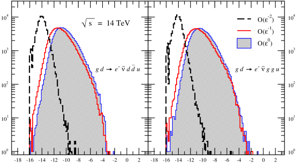
Figure 3: The distribution of the relative error in the leading-color virtual cross section for two subprocesses, $gd\rightarrow e^{-}\bar{\nu}d\bar{d}u$ and $gd\rightarrow e^{-}\bar{\nu}ggu$. The phase-space points are selected in the same way as those used to compute cross sections at the LHC. The horizontal axis is the logarithm of the relative error (6) between an evaluation by BlackHat, running in production mode, and a target expression evaluated using higher precision with at least $32$ decimal digits (or up to $64$ decimal digits for unstable points). The vertical axis shows the number of events out of 100,000 with the corresponding error. The dashed (black) line shows the $1/\epsilon^{2}$ term; the solid (red) curve, the $1/\epsilon$ term; and the shaded (blue) curve, the finite ($\epsilon^{0}$) term.

In fig. 3, we illustrate the numerical stability of the leading-color virtual interference term (or squared matrix element), $d\sigma_{V}$, summed over colors and over all helicity configurations for two subprocesses, $gd\rightarrow e^{-}\bar{\nu}d\bar{d}u$ and $gd\rightarrow e^{-}\bar{\nu}ggu$. (The grid here has been adapted to each of the subprocesses individually, instead of to the sum over subprocesses.) We have checked that the other subprocesses are similarly stable. The horizontal axis of fig. 3 shows the logarithmic error,

$$\log_{10}\left(\frac{|d\sigma_{V}^{\rm num}-d\sigma_{V}^{\rm target}|}{|d\sigma_{V}^{\rm target}|}\right),$$ (6)

for each of the three components: $1/\epsilon^{2}$, $1/\epsilon^{1}$ and $\epsilon^{0}$, where $\epsilon=(4-D)/2$ is the dimensional regularization parameter. The targets have been computed by BlackHat using multiprecision arithmetic with at least $32$ decimal digits, and $64$ if the point is deemed unstable. The overwhelming majority (99.9%) of events are computed to better than one part in $10^{4}$ — that is, to the left of the ‘$-4$’ mark on the horizontal axis.

We have also examined distributions in which each bin is weighted by the requisite squared matrix element and Jacobian factors. We find that they have quite similar shapes to the unweighted distributions shown in fig. 3. This implies that the few events with a relative error larger than $10^{-4}$ make only a small contribution to the total cross section. We have verified that the difference between normal and high-precision evaluation in the total cross section, as well as bin by bin for all distributions studied, is at least three orders of magnitude smaller than the corresponding numerical integration error.

II.5 Real-Emission Corrections

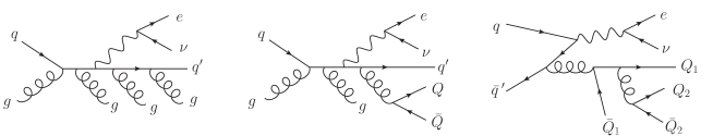
Figure 4: Representative diagrams for the eight-point tree-level amplitudes, $qg\rightarrow e\nu\,q^{\prime}\!ggg$, $qg\rightarrow e\nu\,q^{\prime}\!gQ\bar{Q}$, and $q\bar{q}^{\prime}\rightarrow e\nu\,Q_{1}\bar{Q}_{1}Q_{2}\bar{Q}_{2}$. The $e\nu$ pair couples to the quarks via a $W$ boson.

In addition to the virtual corrections to the cross section provided by BlackHat, an NLO calculation also requires the real-emission corrections to the LO process. These terms arise from tree-level amplitudes with one additional parton: an additional gluon, or a quark–antiquark pair replacing a gluon. Representative real-emission diagrams are shown in fig. 4. Infrared singularities develop when the extra parton momentum is integrated over phase-space regions unresolved by the jet algorithm or jet cuts. The resulting singular integrals cancel against singular terms in the virtual corrections, and against counter-terms associated with the evolution of parton distributions. As mentioned above, to carry out these cancellations, we use the Catani–Seymour dipole subtraction method CS as implemented AutomatedAmegic in the program AMEGIC++ Amegic , which is part of the SHERPA framework Sherpa . This implementation of dipole subtraction has already been tested AutomatedAmegic in explicit comparisons against the DISENT program PrivateSeymour .

The implementation introduces two free parameters, $\alpha_{\rm cut}$ and $\alpha_{\rm dipole}$. The first, $\alpha_{\rm cut}$, parametrizes the volume of phase space to be cut out around the soft or collinear singularity. From an analytic point of view, $\alpha_{\rm cut}$ could be taken to zero, as the cancellation of counter-terms against the matrix element’s singularities is exact. In numerical implementations, however, round-off error can spoil this cancellation. Previous studies have shown that the final result is independent of this cut-off parameter once it is sufficiently small AutomatedAmegic . We use $\alpha_{\rm cut}=10^{-8}$.

The second parameter, $\alpha_{\rm dipole}$, characterizes a common modification of subtraction terms in phase space away from the singularity alphadipole , restricting the support of a given subtraction term to the vicinity of its singularity. This allows the program to compute only a subset of dipole terms, as many will now be identically zero at a given phase-space point. Because the number of dipole terms is large (scaling as $m^{3}$ for processes containing $m$ partons), this reduces the computational burden considerably. We run our code with several different values of $\alpha_{\rm dipole}$, and check the independence of the final result on the value of $\alpha_{\rm dipole}$ ($0<\alpha_{\rm dipole}\leq 1$). For example, the LHC $W^{-}$ results for $\alpha_{\rm dipole}=0.03$ agree with those for $\alpha_{\rm dipole}=0.01$ to better than half a percent, within the integration errors. We have also run a large number of other lower-statistics checks demonstrating that cross sections are independent of the choice of $\alpha_{\rm dipole}$. Our default choice for the LHC is $\alpha_{\rm dipole}=0.03$, while for the Tevatron it is $\alpha_{\rm dipole}=0.01$.

II.6 Phase-Space Integration

Along with the automated generation of matrix elements and dipole terms, SHERPA also provides Monte Carlo integration methods. The phase-space generator combines a priori knowledge about the behavior of the integrands in phase space with self-adaptive integration methods. It employs a multi-channel method in the spirit of ref. MultiChannel . Single channels (phase-space parametrizations) are generated by AMEGIC++ together with the tree-level matrix elements. Each parametrization reflects the structure of a Feynman amplitude, roughly reproducing its resonances, decay kinematics, and its soft and collinear structure. The most important phase-space parametrizations, determined by the adapted relative weight within the multi-channel setup, are further refined using Vegas Vegas .

The phase-space optimization (adaptation of channel weights and Vegas grids) is performed in independent runs before the actual computation starts. The optimization is done on the sum of all contributing parton-level processes. We refer collectively to all the parameters of the optimization as the integration grid. Separate integration grids are constructed for the LO terms and for the real-emission contributions. To integrate the virtual contributions, we re-use the grid constructed for the LO terms. This procedure avoids the computational expense of evaluating the virtual terms merely for grid construction. The virtual to LO ratio is sufficiently flat across phase space that this results in only a slight inefficiency when evaluating distributions.

Following the initialization phase, the integration grids are frozen. In the ensuing production phase, we sample over subprocesses so that only a single parton-level subprocess is evaluated per phase-space point, selected with a probability proportional to its contribution to the total cross section. We choose to integrate the real-emission terms over about $10^{8}$ phase-space points, the leading-color virtual parts over $2\times 10^{6}$ phase-space points and the subleading-color virtual parts over $10^{5}$ phase-space points. The LO and real-subtraction pieces are run separately with $10^{7}$ points each. These numbers are chosen to achieve a total integration error of half a percent or less. For a given choice of scale $\mu$, they give comparable running times for the real-emission and virtual contributions. Running times for leading- and subleading-color virtual contributions are also comparable.

II.7 Couplings and Parton Distributions

We work to leading order in the electroweak coupling and approximate the Cabibbo-Kobayashi-Maskawa (CKM) matrix by the unit matrix. This approximation causes a rather small change in total cross sections for the cuts we impose, as estimated by LO evaluations using the full CKM matrix. At the Tevatron, the full CKM results are about one percent smaller than with the unit CKM matrix; the difference is even smaller at the LHC. We express the $W$-boson couplings to fermions using the Standard Model input parameters shown in table 1. The parameter $g_{w}^{2}$ is derived from the others via,

$$g_{w}^{2}={4\pi\alpha_{\rm QED}(M_{Z})\over\sin^{2}\theta_{W}}\,.$$ (7)

parameter	value
$\alpha_{\rm QED}(M_{Z})$	$1/128.802\;$
$M_{W}$	$\;80.419$ GeV
$\sin^{2}\theta_{W}$	$\;0.230\;$
$\Gamma_{W}$	$2.06$ GeV
$g^{2}_{w}$	0.4242 (calculated)

Table 1: Electroweak parameters used in this work.

We use the CTEQ6M CTEQ6M parton distribution functions (PDFs) at NLO and the CTEQ6L1 set at LO. The value of the strong coupling is fixed accordingly, such that $\alpha_{S}(M_{Z})=0.118$ and $\alpha_{S}(M_{Z})=0.130$ at NLO and LO respectively. We evolve $\alpha_{S}(\mu)$ using the QCD beta function for five massless quark flavors for $\mu<m_{t}$, and six flavors for $\mu>m_{t}$. (The CTEQ6 PDFs use a five-flavor scheme for all $\mu>m_{b}$, but we use the SHERPA default of six-flavor running above top-quark mass; the effect on the cross section is very small, on the order of one percent at larger scales.) At NLO we use two-loop running, and at LO, one-loop running.

II.8 Kinematics and Observables

As our calculation is a parton-level one, we do not apply corrections due to non-perturbative effects such as those induced by the underlying event or hadronization. CDF has studied WCDF these corrections at the Tevatron, and found they are under ten percent when the $n^{\rm th}$ jet $E_{T}$ is below 50 GeV, and under five percent at higher $E_{T}$.

For completeness we state the definitions of standard kinematic variables used to characterize scattering events. We denote the angular separation of two objects (partons, jets or leptons) by

$$\Delta R=\sqrt{(\Delta\phi)^{2}+(\Delta\eta)^{2}}\,,$$ (8)

with $\Delta\phi$ the difference in the azimuthal angles, and $\Delta\eta$ the difference in the pseudorapidities. The pseudorapidity $\eta$ is given by

$$\eta=-\ln\left(\tan\frac{\theta}{2}\right)\,,$$ (9)

where $\theta$ is the polar angle with respect to the beam axis.

The transverse energies of massless outgoing partons and leptons, $E_{T}=\sqrt{p_{x}^{2}+p_{y}^{2}}$, can be summed to give the total partonic transverse energy, ${\hat{H}}_{T}$, of the scattering process,

$${\hat{H}}_{T}=\sum_{p}E_{T}^{p}+E_{T}^{e}+E_{T}^{\nu}\,.$$ (10)

All partons $p$ and leptons are included in ${\hat{H}}_{T}$, whether or not they are inside jets that pass the cuts. We shall see in later sections that the variable ${\hat{H}}_{T}$ represents a good choice for the renormalization and factorization scale of a given event. Although the partonic version is not directly measurable, for practical purposes as a scale choice, it is essentially equivalent (and identical at LO) to the more usual jet-based total transverse energy,

$$H_{T}=\sum_{j}E_{T,j}^{\rm jet}+E_{T}^{e}+E_{T}^{\nu}\,.$$ (11)

The partonic version ${\hat{H}}_{T}$ has the advantage that it is independent of the cuts; thus, loosening the cuts will not affect the value of the matrix element, because a renormalization scale of ${\hat{H}}_{T}$ will be unaffected. On the other hand, we use the jet-based quantity $H_{T}$, which is defined to include only jets passing all cuts, to compute observable distributions. Note that for $W\,\!+\,n$-jet production at LO, exactly $n$ jets contribute to eq. (11); at NLO either $n$ or $n+1$ jets may contribute.

The jet four-momenta are computed by summing the four-momenta of all partons that are clustered into them,

$$p^{\rm jet}_{\mu}=\sum_{i\in{\rm jet}}p_{i\mu}\,.$$ (12)

The transverse energy is then defined in the usual way, as the energy multiplied by the momentum unit vector projected onto the transverse plane,

$$E_{T}^{\rm jet}=E^{\rm jet}\sin\theta^{\rm jet}\,.$$ (13)

The total transverse energy as defined in eq. (11) is intended to match the experimental quantity, given by the sum,

$$H_{T}^{\rm exp}=\sum_{j}E_{T,j}^{\rm jet}+E_{T}^{e}+{{\raise 0.91666pt\hbox to7.95831pt{\hss/\hss}\hbox to0.0pt{\hss$E$}}}_{T}\,,$$ (14)

where ${{\raise 0.91666pt\hbox to7.95831pt{\hss/\hss}\hbox to0.0pt{\hss$E$}}}_{T}$ is the missing transverse energy. Jet invariant masses are defined by

$$M^{2}_{ij}=(p^{\rm jet}_{i}+p^{\rm jet}_{j})^{2}\,,$$ (15)

and the jets are always labeled $i,j=1,2,3,\ldots$ in order of decreasing transverse energy $E_{T}$, with $1$ being the leading (hardest) jet. The transverse mass of the $W$-boson is computed from the kinematics of its decay products, $W\rightarrow e\nu_{e}$,

$$M_{T}^{W}=\sqrt{2E_{T}^{e}E_{T}^{\nu}(1-\cos(\Delta\phi_{e\nu}))}\,.$$ (16)

II.9 Checks

We have carried out numerous checks on our code, ranging from checks of the basic primitive amplitudes in specific regions of phase space to overall checks of total and differential distributions against existing codes. We have compared our results for the total cross section for $W\,\!+\,1,2$-jet production (at a fixed scale $\mu=M_{W}$) with the results obtained from running MCFM MCFM . Because the publicly available version of MCFM does not allow a cut in $M_{T}^{W}$ we eliminated this cut in the comparison. (We had previously compared the matrix elements used in the latter code obtained from ref. Zqqgg , to the results produced purely numerically in BlackHat.) Agreement at LO and NLO for $W\,\!+\,1$-jet production at the LHC is good to a per mille level. For $W\,\!+\,2$-jet production, at LO we find agreement with MCFM within a tenth of a percent, while at NLO, where the numerical integration is more difficult, we find agreement to better than half a percent. We find the same level of agreement at NLO at the Tevatron, using a different set of cuts.

We have carried out extensive validations of our code at a finer-grained level. We have confirmed that the code reproduces the expected infrared singularities (poles in $\epsilon$) for the primitive amplitudes and the full color-dressed one-loop amplitudes OneloopIR ; CS . We have also confirmed that the poles in $\epsilon$ in the full virtual cross section cancel against those found in the integrated real-subtraction terms AutomatedAmegic .

We checked various factorization limits, both two-particle (collinear) and multi-particle poles. These factorization checks are natural in the context of on-shell recursion. This method constructs the rational terms using a subset of the collinear and multi-particle factorization poles; the behavior in other channels constitutes an independent cross check. For the leading-color primitive amplitudes, we verified that all factorization limits of the amplitudes are correct. (We also checked that all spurious poles cancel.) For the subleading-color primitive amplitudes, we verified the correct behavior as any two parton momenta become collinear. We also checked at least one collinear limit for each partial amplitude.

We had previously computed the leading-color amplitudes for the subprocess (3) in ref. ICHEPBH . Ellis et al. W3EGKMZ confirmed these values, and also computed the subleading-color primitive amplitudes. This evaluation used $D$-dimensional generalized unitarity DdimUnitarity ; DdimUnitarityRecent ; GKM , a decomposition of the processes in eqs. (2) and (3) into primitive amplitudes qqggg ; Zqqgg , and the OPP formalism for obtaining coefficients of basis integrals OPP . We have compared the subleading-color primitive amplitudes at a selected phase-space point to the numerical values reported in ref. W3EGKMZ , and find agreement, up to convention-dependent overall phases. Van Hameren, Papadopoulos, and Pittau (HPP) recently computed HPP the full helicity- and color-summed virtual cross section for the subprocess $u\bar{d}\to W^{+}ggg$ at another phase-space point, for an undecayed on-shell $W$ boson and including (small) virtual top-quark contributions. They used the OPP formalism and the CutTools CutTools and HELAC-1L HELAC ; HPP codes. We have compared the full squared matrix element to the result produced by the HPP code, with the top-quark contributions removed. We find agreement with their value of the ratio of this quantity to the LO cross section. We have also found agreement with matrix-element results from the same code, allowing the $W$ boson to decay to leptons, as in our setup. We give numerical values of the squared matrix elements for an independent set of subprocesses, evaluated at a different phase-space point, in an appendix.

As mentioned earlier, we verified that the computed values of the virtual terms are numerically stable when integrated over grids similar to those used for computing the cross section and distributions. We also checked that our integrated results do not depend on $\alpha_{\rm dipole}$, the unphysical parameter controlling the dipole subtraction alphadipole , within integration uncertainties.

III Tevatron Results

In this section we present next-to-leading order results for $W\,\!+\,3$-jet production in $p\bar{p}$ collisions at $\sqrt{s}=1.96$ TeV, the experimental configuration at the Tevatron. We decay the $W$ bosons into electrons or positrons (plus neutrinos) in order to match the CDF study WCDF . In our earlier Letter PRLW3BH , we presented results for the third jet’s transverse energy ($E_{T}$) distribution as well as the total transverse energy ($H_{T}$) distribution. Those calculations employed a particular leading-color approximation for the virtual terms PRLW3BH . As discussed in section VIII, this approximation is an excellent one, accurate to within three percent. In the present paper, we give complete NLO results for a larger selection of distributions, including all subleading-color terms. It would be interesting to compare the new distributions with experimental results from both CDF and D0, as they become available.

We use the same jet cuts as in the CDF analysis WCDF ,

$$E_{T}^{\rm jet}>20\,{\rm GeV}\,,\hskip 28.45274pt\quad|\eta^{\rm jet}|<2\,.$$ (17)

Following ref. WCDF , we quote total cross sections using a tighter jet cut, $E_{T}^{\rm jet}>25\,{\rm GeV}$. We order jets by $E_{T}$. Both electron and positron final states are counted, using the same lepton cuts as CDF,

$$E_{T}^{e}>20\,{\rm GeV}\,,\hskip 28.45274pt|\eta^{e}|<1.1\,,$$

$${{\raise 0.91666pt\hbox to7.95831pt{\hss/\hss}\hbox to0.0pt{\hss$E$}}}_{T}>30\,{\rm GeV}\,,\hskip 28.45274ptM_{T}^{W}>20\,{\rm GeV}.$$ (18)

(We replace the ${{\raise 0.91666pt\hbox to7.95831pt{\hss/\hss}\hbox to0.0pt{\hss$E$}}}_{T}$ cut by one on the neutrino $E_{T}^{\nu}$.) CDF also imposes a minimum $\Delta R$ between the charged decay lepton and any jet; the effect of this cut, however, is undone by a specific acceptance correction CDFThesis . Accordingly, we do not impose it.

For the LO and NLO results for the Tevatron we use an event-by-event common renormalization and factorization scale, set equal to the $W$ boson transverse energy,

$$\mu=E_{T}^{W}\equiv\sqrt{M_{W}^{2}+p_{T}^{2}(W)}\,.$$ (19)

To estimate the scale dependence we choose five values: $\mu/2,\mu/\sqrt{2},\mu,\sqrt{2}\mu,2\mu$.

number of jets	CDF	LO	NLO
1	$\;53.5\pm 5.6\;$	$41.40(0.02)^{+7.59}_{-5.94}$	$\;57.83(0.12)^{+4.36}_{-4.00}\;$
2	$6.8\pm 1.1$	$6.159(0.004)^{+2.41}_{-1.58}$	$7.62(0.04)^{+0.62}_{-0.86}$
3	$0.84\pm 0.24$	$0.796(0.001)^{+0.488}_{-0.276}$	$0.882(0.005)^{+0.057}_{-0.138}$

Table 2: Total inclusive cross sections, in pb, for $W\,\!+\,n$ jets produced at the Tevatron with $W\to e\nu$ and $E_{T}^{n\rm th\hbox{-}jet}>25$ GeV, using the experimental cuts of ref. WCDF . The first column gives the experimental results as measured by CDF. The experimental statistical, systematic and luminosity uncertainties have been combined in quadrature. The second column shows LO results, and the third column the complete NLO results. In each case, the scale dependence is quoted in super- and subscripts and the numerical integration uncertainties in parentheses.

The CDF analysis used the JETCLU cone algorithm JETCLU with cone radius $R=0.4$. This algorithm is not generally infrared safe at NLO, so we use the seedless cone algorithm SISCone SISCONE instead. Like other cone-type algorithms, SISCone gives rise to jet-production cross sections that can depend on an overlap threshold or merging parameter, here called $f$. No dependence on $f$ can develop at LO, because such dependence would require the presence of partons in the overlap of two cones. The $W\,\!+\,1$-jet production cross section likewise cannot depend on $f$ at NLO. We set this parameter to $0.5$. (Unless stated otherwise we take this algorithm and parameter choice as our default.)

We expect similar results at the partonic level from any infrared-safe cone algorithm. For $W\,\!+\,1,2$-jet production we have confirmed that distributions using SISCone are within a few percent of those obtained with MCFM using the midpoint cone algorithm Midpoint . (The midpoint algorithm is infrared-safe at NLO for $W\,\!+\,1,2$-jet production, but not for $W\,\!+\,3$-jet production SISCONE .) The algorithm dependence of $W\,\!+\,3$-jet production at the Tevatron at NLO has also been discussed recently by Ellis et al. EMZ2 .

In table 2, we collect the results for the total cross section, comparing CDF data to the LO and NLO theoretical predictions computed using BlackHat and SHERPA. In both cases these are parton-level cross sections. Results from more sophisticated (“enhanced”) LO analyses incorporating parton showering and matching schemes Matching ; MLMSMPR ; LOComparison may be found in ref. WCDF ; however, large scale dependences still remain. (These calculations make different choices for the scale variation and are not directly comparable to the LO parton-level predictions given here.) As in the experimental analysis, we sum the $W^{-}$ and $W^{+}$ cross sections, which are identical at the Tevatron (for forward-backward symmetric acceptance cuts).

We have also computed the $W\,\!+\,2$-jet and $W\,\!+\,3$-jet total cross sections at NLO with a larger merging parameter, $f=0.75$. (CDF uses a value of $f=0.75$ WCDF , but for a different, infrared-unsafe algorithm, JETCLU.) The value of the NLO $W\,\!+\,3$-jet production cross section of $0.882$ pb in table 2 then increases to $0.917$ pb (about 4%). The $W\,\!+\,2$-jet production cross section shows a more modest increase from $7.62$ pb to $7.69$ pb (about 1%). Distributions, as for example the ones shown in fig. 5 (see also table 3), follow a similar bin-by-bin dependence on $f$.

$E_{T}^{\rm 3rd\hbox{-}jet}$	$d\sigma/dE_{T}^{\rm 3rd\hbox{-}jet}$ (pb/GeV)
	CDF	LO	NLO
20-25	$\;0.184\pm 0.0394\;$	$\;0.131^{+0.0769}_{-0.0443}\;$	$\;0.160^{+0.0205}_{-0.0277}\;$
25-30	$\;0.087\pm 0.0268\;$	$\;0.066^{+0.0393}_{-0.0224}\;$	$\;0.077^{+0.0075}_{-0.0126}\;$
30-35	$\;0.037\pm 0.0153\;$	$\;0.036^{+0.0216}_{-0.0123}\;$	$\;0.041^{+0.0036}_{-0.0068}\;$
35-45	$\;0.020\pm 0.0125\;$	$\;0.017^{+0.0103}_{-0.0058}\;$	$\;0.018^{+0.0009}_{-0.0027}\;$
45-80	$\;0.0015\pm 0.00177\;$	$\;0.0032^{+0.00207}_{-0.00114}\;$	$\;0.0031^{+0.00015}_{-0.00041}\;$

Table 3: The differential cross sections, $d\sigma(p\bar{p}\rightarrow e\nu+\geq 3$-jets)$/dE_{T}^{3\rm rd\hbox{-}jet}$, for $W\,\!+\,3$-jet production at the Tevatron using the experimental cuts (17) and (18) of ref. WCDF . This table corresponds to the values plotted in fig. 5.

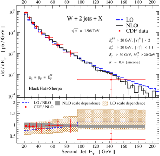
Figure 5: The measured cross section, $d\sigma(p\bar{p}\rightarrow e\nu+\geq n$-jets)$/dE_{T}^{n\rm th\hbox{-}jet}$, for inclusive $W\,\!+\,n$-jet production, compared to full NLO predictions for $n=2,3$. In the upper panels the NLO distribution is the solid (black) histogram, and CDF data points are the (red) points, whose inner and outer error bars, respectively, denote the statistical and total uncertainties (excluding the luminosity error) on the measurements added in quadrature. The LO predictions are shown as dashed (blue) lines. The thin vertical lines in the center of each bin (where visible) give the numerical integration errors for that bin. Each lower panel shows the distribution normalized to the full NLO prediction, using the CDF experimental bins (that is, averaging over bins in the upper panel). The scale-dependence bands are shaded (gray) for NLO and cross-hatched (brown) for LO.

In fig. 5, we compare the $E_{T}$ distribution of the second- and third-most energetic jets in CDF data WCDF to the NLO predictions for $W\,\!+\,2$-jet and $W\,\!+\,3$-jet production, respectively. For convenience, in table 3 we collect the data used to construct the third-jet $E_{T}$ plot in fig. 5. We include scale-dependence bands obtained as described above. The experimental statistical and systematic uncertainties (excluding an overall luminosity uncertainty of 5.8%) have been combined in quadrature. The upper panels of fig. 5 show the distribution itself, while the lower panels show the ratio of the LO value and of the data to the NLO result for the central value of $\mu=E_{T}^{W}$. Note that we normalize here to the NLO result, not to LO as done elsewhere. The LO/NLO curve in the bottom panel represents the inverse of the so-called $K$ factor (NLO to LO ratio).

We do not include PDF uncertainties in our analysis. For $W\,\!+\,1,2$-jet production at the Tevatron these uncertainties have been estimated in ref. WCDF . For these processes, they are smaller than uncertainties associated with NLO scale dependence at low jet $E_{T}$, but larger at high $E_{T}$.

For reference, we also show the LO distributions and corresponding scale-dependence bands. The NLO predictions match the data very well, and uniformly (without any difference in slope) in all but the highest $E_{T}$ experimental bin. The central values of the LO predictions, in contrast, have different shapes from the data. In the upper panels, we have used 5 GeV bins to plot the predictions, and have superposed the data points, although CDF used different bins in their analysis. In the lower panel, which shows the ratio of the LO prediction, and of the data, to the NLO prediction, we have used the experimental bins, which are wider at higher $E_{T}$. A very similar plot was given previously PRLW3BH , based on a particular leading-color approximation. As we discuss in section VIII, those results differ only slightly from the complete NLO results presented here.

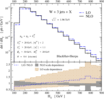
Figure 6: Theoretical predictions for the $H_{T}$ distribution in $W\,\!+\,3$-jet production at the Tevatron. The LO prediction is shown by a dashed (blue) line; the NLO one by a solid (black) one. The upper panel shows the distribution itself, while the lower panel shows the distributions and scale-dependence bands, cross-hatched (brown) for LO and solid (gray) for NLO, normalized to the NLO prediction for $\mu=E_{T}^{W}$. The numerical integration errors, indicated by thin vertical lines in the upper panel, are noticeable only in the tail.

In fig. 6, we show the distribution for the total transverse energy $H_{T}$, given in eq. (14). This quantity has been used in top-quark studies, and will play an important role in searches for decays of heavy new particles at the LHC. The upper panel shows the LO and NLO predictions for the distribution, and the lower panel their ratio. The NLO scale-dependence band, as estimated using five points, ranges from $\pm 20\%$ around its central value at low $H_{T}$ to $\pm 5\%$ around 400 GeV, and back to around $\pm 10\%$ at 800 GeV. The band is accidentally narrow at energies near the middle of graph, because the curves associated with the five $\mu$ values converge as the $H_{T}$ value rises from lower values towards the middle ones. (The fluctuations visible in the tail of the distribution are a reflection of the limited statistics for the Monte Carlo integration, as we show a larger dynamical range than in the $E_{T}$ spectrum.) The shape of the LO distribution is noticeably different, for any of the $\mu$ values, from that at NLO. At low $H_{T}$, the central LO prediction is 20% below the NLO central value, whereas at the largest $H_{T}$ it is nearly 50% higher. Thus for $\mu=E_{T}^{W}$ the NLO correction cannot be characterized by a constant $K$ factor (ratio of NLO to LO results). We will address some of the reasons for the difference in shape in the following section. We note that the NLO scale-dependence band has a somewhat different appearance from the corresponding figure in ref. PRLW3BH , because the latter used wider bins at large $H_{T}$ and had larger integration errors.

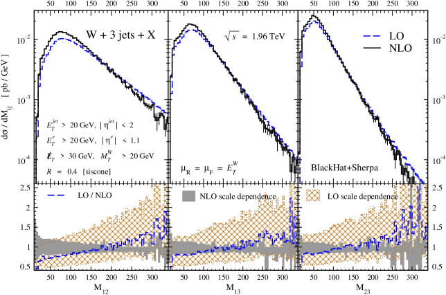
Figure 7: LO and NLO predictions for the di-jet invariant mass distributions $M_{ij}$ (in GeV) in $W\,\!+\,3$-jet production at the Tevatron. The histograms and bands have the same meaning as in figs. 5 and 6.

In fig. 7, we show the distributions for the three di-jet invariant masses we can form: hardest and middle jet $M_{12}$, hardest and softest jet $M_{13}$, and middle and softest jet $M_{23}$. The NLO scale-dependence bands are somewhat broader than for the $E_{T}$ or $H_{T}$ distributions. The distributions become increasingly steep as we move from masses of hardest to softer jets. That gross feature is unaltered in passing from LO to NLO, although each distribution falls off somewhat faster at NLO, as was the case for $H_{T}$.

IV Choosing Scales

The renormalization and factorization scales are not physical scales. As such, physical quantities should be independent of them. They arise in theoretical calculations as artifacts of defining $\alpha_{S}$ and the parton distributions, respectively. We will follow the usual practice and choose the two to be equal, $\mu_{R}=\mu_{F}=\mu$. The sensitivity of a perturbative result to the common scale is due to the truncation of the perturbative expansion; this dependence would be canceled by terms at higher orders. NLO calculations greatly reduce this dependence compared to LO results, but of course do not eliminate it completely. In practice, we must therefore choose this scale. Intuitively, we would expect a good choice for $\mu$ to be near a “characteristic” momentum scale $p$ for the observable we are computing, in order to minimize logarithms in higher-order terms of the form $\ln(\mu/p)$. The problem is that complicated processes such as $W\,\!+\,2,3$-jet production have many intrinsic scales, and it is not clear we can distill them into a single number. For any given point in the fully-differential cross section, there is a range of scales one could plausibly choose. One could choose a fixed scale $\mu$, the same for all events. However, because there can be a large dynamic range in momentum scales (particularly at the LHC, where jet transverse energies well above $M_{W}$ are not uncommon), it is natural to pick the scale $\mu$ dynamically, on an event-by-event basis, as a function of the observable or unobservable parameters of an event.

A particularly good choice of scale might minimize changes in shape of distributions from LO to NLO, such as those visible in figs. 6 and 7. Such a choice might in turn make it possible for LO programs incorporating parton showering and hadronization Matching ; MLMSMPR ; LOComparison to be more easily reweighted to reflect NLO results.

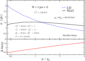
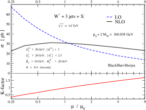
Figure 8: The scale dependence of the cross section for $W\,\!+\,3$-jet production at the Tevatron is shown on the left, as a function of the common renormalization and factorization scale $\mu$, with $\mu_{0}=M_{W}$. Similar curves for $W^{-}\,\!+\,3$-jet production at the LHC are shown on the right, except that $\mu_{0}=2M_{W}$. In each case, the lower panel shows the $K$ factor.

Before turning to dynamical scales and kinematic distributions, let us first examine how the total cross section depends on a fixed scale. In fig. 8 we display this dependence for the Tevatron and the LHC (left and right respectively). We vary the scale between $\mu=M_{W}/2$ and $4M_{W}$ for the Tevatron, and between $M_{W}/2$ and $16M_{W}$ for the LHC. We must be careful to vary the scale in a ‘sensible’ range. For the NLO calculation in particular, we do not wish to reintroduce large logarithms of scales. The figure shows the characteristic increasing-and-decreasing of the NLO prediction (see e.g. refs. CTEQscales ; CHS ) as well as the monotonicity of the LO one. It also shows a substantial reduction in scale dependence going from LO to NLO. The lower panels show the $K$ factor. The large sensitivity of the LO cross section to the choice of scale implies a similar large dependence in this ratio.

We thus see that, as expected, the total cross sections at NLO are much less sensitive to variations of the scale than at LO. We now turn to the scale dependence of kinematic distributions. In this case the $K$ factor will not only be sensitive to the scale chosen, but it will in general depend on the kinematic variable. We will see that a poor choice of scale can lead to problems not only at LO, but also at NLO, especially in the tails of distributions.

Figure 9: The $E_{T}$ distribution of the second jet at LO and NLO, for two dynamical scale choices, $\mu=E_{T}^{W}$ (left plot) and $\mu={\hat{H}}_{T}$ (right plot). The histograms and bands have the same meaning as in previous figures. The NLO distribution for $\mu=E_{T}^{W}$ turns negative beyond $E_{T}=475$ GeV.

The sensitivity to a poor scale choice is already noticeable at the Tevatron, in the shape differences between LO and NLO predictions visible in figs. 6 and 7. However, it becomes more pronounced at the LHC because of the larger dynamical range of available jet transverse energies. We can diagnose particularly pathological choices of scale using the positivity of the NLO cross section: too low a scale at NLO will make the total cross section unphysically negative.

This diagnostic can be applied bin by bin in distributions. For example, in fig. 9 we show the $E_{T}$ distribution of the second-most energetic jet of the three, at the LHC. In the left plot we choose the scale to be the $W$ transverse energy $E_{T}^{W}$ (defined in eq. (19)) used earlier in the Tevatron analysis. Near an $E_{T}$ of 475 GeV, the NLO prediction for the differential cross section turns negative! This is a sign of a poor scale choice, which has re-introduced large enough logarithms of scale ratios to overwhelm the LO terms at that jet $E_{T}$. Its inadequacy is also indicated by the large ratio of the LO to NLO distributions at lower $E_{T}$, and in the rapid growth of the NLO scale-dependence band with $E_{T}$. In contrast, the right panel of fig. 9 shows that ${\hat{H}}_{T}$ (defined in eq. (10)) provides a sensible choice of scale: the NLO cross section stays positive, and the ratio of the LO and NLO distributions, though not completely flat, is much more stable.

Figure 10: Two distinct $W\,\!+\,3$ jet configurations with rather different scales for the $W$ transverse energy. In configuration (a) an energetic $W$ balances the energy of the jets, while in (b) the $W$ is relatively soft. Configuration (b) generally dominates over (a) when the jet transverse energies get large.

Why is $\mu=E_{T}^{W}$ such a poor choice of scale for the second jet $E_{T}$ distribution, compared with $\mu={\hat{H}}_{T}$? (For an independent, but related discussion of this question, see ref. Bauer .) Consider the two distinct types of $W\,\!+\,3$ jet configurations shown in fig. 10. If configuration (a) dominated, then as the jet $E_{T}$ increased, $E_{T}^{W}$ would increase along with it, by conservation of transverse momentum. However, in configuration (b), the bulk of the transverse momentum can be balanced between the first and second jet, with the $W$ and the third jet remaining soft. In the tail of the second-jet $E_{T}$ distribution, configuration (b) is highly favored kinematically, because it implies a much smaller partonic center-of-mass energy. Because $E_{T}^{W}$ remains small, the wrong scale is being chosen in the tail. Evidence for the dominance of configuration (b) over (a) in $W\,\!+\,2$-jet production can be found in ref. Bauer , which shows that the two jets become almost back to back as the jet $E_{T}$ cut rises past $M_{W}$. The negative NLO cross section in the left panel of fig. 9 provides evidence of the same domination in $W\,\!+\,3$-jet production.

However, configuration (b) also tends to dominate in the tails of generic multi-jet distributions, such as $H_{T}$ or $M_{ij}$, in which large jet transverse energies are favored. The reason is that for jet transverse energies well above $M_{W}$, the $W$ behaves like a massless vector boson, and so there is a kinematic enhancement when it is soft, as in configuration (b). Exceptions would be in distributions such as the transverse energy of the $W$ itself, or of its decay lepton, which kinematically favor configuration (a) in their tails.

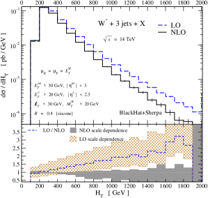
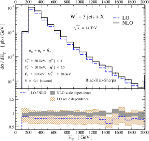
Figure 11: The $H_{T}$ distribution for $W^{-}\,\!+\,3$-jet production at the LHC. The scale choices $\mu=E_{T}^{W}$ and $\mu={\hat{H}}_{T}$ are shown, respectively, on the left and the right. The histograms and bands have the same meaning as in previous figures.

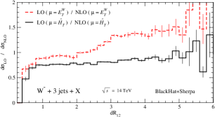
Figure 12: Ratios of LO to NLO predictions for the distributions in the di-jet invariant mass (left panel) and $\Delta R$ separation (right panel) for the leading two jets in $W^{-}\,\!+\,3$-jet production at the LHC. In each panel, the dashed (red) line gives the scale choice $\mu=E_{T}^{W}$, while the solid (black) line gives the (much flatter) ratio for $\mu={\hat{H}}_{T}$.

In contrast to $\mu=E_{T}^{W}$, the scale $\mu={\hat{H}}_{T}$ becomes large in the tails of generic multi-jet transverse-energy distributions. For the distribution of the second jet $E_{T}$, this is evident from the close agreement between LO and NLO values, shown in the right panel of fig. 9. The same features are evident, though less pronounced, in the $H_{T}$ distributions shown in fig. 11. The left plot is again for $\mu=E_{T}^{W}$, and the right plot for $\mu={\hat{H}}_{T}$. The shapes of the LO and NLO distributions for $\mu=E_{T}^{W}$ are quite different; the ratio displayed varies from around 1 at $H_{T}$ of 200 GeV to around 2 at $H_{T}$ near 1200 GeV. In contrast, the ratio for $\mu={\hat{H}}_{T}$ is nearly flat.

These features are not special to the $H_{T}$ distribution itself. For example, fig. 12 displays the ratio of LO to NLO predictions for two other $W\,\!+\,3$-jet distributions for the two scale choices. The left panel shows the ratios for the leading di-jet mass, while the right panel shows ratios for the leading $\Delta R$ distribution. Once again the ratios for $\mu={\hat{H}}_{T}$ have a much milder dependence than those for $\mu=E_{T}^{W}$.

As we shall see further in the next section, the roughly flat ratio for the choice $\mu={\hat{H}}_{T}$ holds for a wide variety of distributions. It does not hold for all: some NLO corrections cannot be absorbed into a simple redefinition of the renormalization scale. The distribution of the second-most energetic jet in fig. 9 provides one example. A second example, discussed below, is the $H_{T}$ distribution for $W^{+}\,\!+\,2$-jet production in the left plot of fig. 15. A third example (not shown) would be the $H_{T}$ distribution for $W\,\!+\,1$-jet production; this case is easy to understand because only configuration (a) (with the second and third jets erased) is available at LO, while configuration (b) can dominate at NLO, so effectively a new subprocess opens up at NLO.

Although the $E_{T}^{W}$ scale choice is a poor one as far as the tails of many distributions are concerned, we note that it does give reasonable results for the Tevatron and LHC total cross sections with our standard jet cuts, which are dominated by modest jet transverse energies. For $\mu=E_{T}^{W}$, the NLO cross section for $W^{-}\,\!+\,3$-jet production at the LHC is $31.37(0.20)^{+0.0}_{-2.47}$ pb, which has much smaller scale variation than the LO result $37.16(0.07)^{+16.35}_{-10.35}$ pb. (The parentheses indicate the integration uncertainties, and subscripts and superscripts the scale variation.) For $\mu={\hat{H}}_{T}$, the NLO value is $27.52(0.14)^{+1.34}_{-2.81}$ pb; the two NLO results are consistent within the scale variation band.

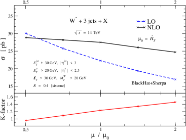
Figure 13: The scale dependence of the cross section for $W^{-}\,\!+\,3$-jet production at the LHC as a function of $\mu/\mu_{0}$, with $\mu_{0}={\hat{H}}_{T}$.

Accordingly, to have a proper description of distributions, we adopt ${\hat{H}}_{T}$ as our default choice of scale for $W\,\!+\,3$-jet production at the LHC. In fig. 13 we display the scale variation of the total cross section, evaluating it at the five scales $\mu_{0}/2,\mu_{0}/\sqrt{2},\mu_{0},\sqrt{2}\mu_{0},2\mu_{0}$ with $\mu_{0}={\hat{H}}_{T}$. As usual, the variation is much smaller at NLO than at LO. Because ${\hat{H}}_{T}$ includes a scalar sum, it is somewhat larger than an “average” momentum transfer. One could choose a scale lower by a fixed ratio, say ${\hat{H}}_{T}/2$. This would shift the LO-to-NLO ratio curves in figs. 11 and 12, for example, up towards a ratio of 1. It would have only a modest effect on the NLO predictions, however, because the scale-dependence curve for the NLO cross section is relatively flat.

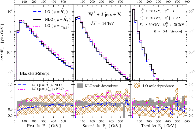
Figure 14: The first, second, and third jet $E_{T}$ distributions for $W^{+}\,\!+\,3$-jet production. The scale choice $\mu=\mu_{\rm had}$ at LO, shown by the dot-dashed (magenta) lines, is compared with the LO and NLO results using our default scale choice $\mu={\hat{H}}_{T}$, shown respectively in the dashed (blue) and solid (black) lines. The scale-dependence bands are shaded (gray) for NLO and cross-hatched (brown) for LO.

It is interesting to compare our default choice $\mu={\hat{H}}_{T}$ with the choice of scale advocated in ref. Bauer on the basis of soft-collinear-effective theory,

$$\mu_{\rm had}^{2}={1\over 4}M_{\rm had}^{2}+M_{W}^{2}\,.$$ (20)

In this equation $M_{\rm had}$ is the invariant mass of the jets. (As explained in ref. Bauer , the factor of $1/4$ is a choice, not dictated by a principle.) With this choice, one can greatly reduce the shift between LO and NLO in $W\,\!+\,2$-jet distributions, compared to more conventional choices such as $\mu=E_{T}^{W}$. We have confirmed that for $W\,\!+\,2$-jet production with a few exceptions, such as the decay lepton transverse energy, the choice $\mu=\mu_{\rm had}$ does fare better than $\mu=E_{T}^{W}$ in bringing LO in line with NLO. How does this choice fare in $W\,\!+\,3$-jet production? To answer this question, we have compared several distributions. In fig. 14, we consider the $E_{T}$ distributions of the first, second and third jets in $W^{+}\,\!+\,3$-jet production at the LHC. We compare the LO results for $\mu={\hat{H}}_{T}$ and $\mu=\mu_{\rm had}$ to the reference NLO results for $\mu={\hat{H}}_{T}$. (Any sensible choice of scale at NLO should give very similar results.) As can be seen from the figure, the choice $\mu={\hat{H}}_{T}$ leads to a somewhat flatter LO to NLO ratio than does $\mu=\mu_{\rm had}$ for the first jet, and performs about as well for the second and third leading jets.

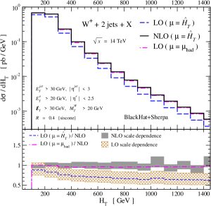
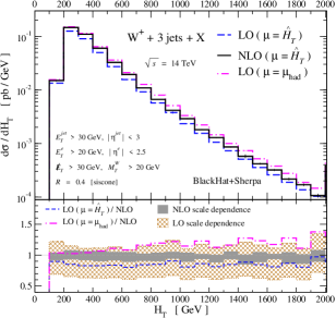
Figure 15: The $H_{T}$ distributions for $W^{+}\,\!+\,2,3$-jet production. LO results for $\mu=\mu_{\rm had}$ are compared with LO and NLO results for $\mu={\hat{H}}_{T}$. The lines and bands have the same meaning as in fig. 14.

It is also instructive to compare the $H_{T}$ distributions for $W\,\!+\,2$-jet and $W\,\!+\,3$-jet production. The left panel of fig. 15 shows the distribution in $W^{+}\,\!+\,2$-jet production; here the scale $\mu=\mu_{\rm had}$ gives an LO result closer to the NLO one. On the other hand, in the right panel, which shows the distribution in $W^{+}\,\!+\,3$-jet production, the choice $\mu={\hat{H}}_{T}$ gives a LO to NLO ratio which is comparably flat to the $\mu=\mu_{\rm had}$ choice.

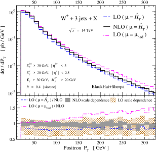
Figure 16: The distribution in the positron transverse momentum for $W^{+}\,\!+\,2,3$-jet production at the LHC. LO results for $\mu=\mu_{\rm had}$ are compared with LO and NLO results for $\mu={\hat{H}}_{T}$. The lines and bands have the same meaning as in fig. 14.

In contrast, examine the positron $p_{T}$ (or $E_{T}$) distribution, shown in fig. 16 for $W^{+}\,\!+\,2,3$-jet production at the LHC. As can be seen in the lower panel of each plot, the choice $\mu={\hat{H}}_{T}$ performs better than $\mu=\mu_{\rm had}$ at LO, in matching the more accurate NLO result at large values of $E_{T}^{e}$. The reason is that large $E_{T}^{e}$ forces the $W$ transverse energy to be large, which in turn favors configuration (a) in fig. 10, in which a relatively low-mass cluster of jets recoils against the $W$ boson. Thus the scale $\mu=\mu_{\rm had}$ drops below the typical momentum transfer in the process.

In summary, both $\mu=\mu_{\rm had}$ and $\mu={\hat{H}}_{T}$ are a great improvement over the scale choice $\mu=E_{T}^{W}$. For some distributions $\mu=\mu_{\rm had}$ is a somewhat better choice at LO than $\mu={\hat{H}}_{T}$, while for other distributions $\mu={\hat{H}}_{T}$ is better. These attributes should not come as a surprise, given the multi-scale nature of jet production.

V Predictions for the LHC

In this section we present the first complete NLO predictions for $W\,\!+\,3$-jet production at the LHC. The initial run of the LHC will almost certainly not be at its full design energy of 14 TeV, but we choose this energy to simplify comparisons to earlier studies. Most of the features visible at 14 TeV would of course remain at the lower energy, such as 10 TeV, of an initial run. The production of $W\,\!+\,3$ jets at the LHC was also studied at NLO in ref. EMZ , however with a set of subprocesses accounting for only 70% of the cross section; for on-shell $W$ bosons; and with a less accurate leading-color approximation than that of ref. PRLW3BH . For our analysis of $W\,\!+\,3$-jet production at the LHC, we use the following kinematical cuts,

$$|\eta^{\rm jet}|<3\,,\hskip 42.67912ptR=0.4\,,\hskip 42.67912pt|\eta^{e}|<2.5\,,\hskip 42.67912ptE_{T}^{e}>20\,\hbox{GeV}\,,\hskip 42.67912pt$$

$$\hskip 85.35826ptE_{T}^{\nu}>30\,\hbox{GeV}\,,\hskip 42.67912ptM_{T}^{W}>20\,\hbox{GeV}\,.\hskip 42.67912pt$$ (21)

We also quote total cross sections with both of the following jet cuts

$$E_{T}^{\rm jet}>30\,{\rm GeV}\hskip 19.91692pt\hbox{and}\hskip 19.91692ptE_{T}^{\rm jet}>40\,{\rm GeV}\,.$$ (22)

We show distributions only using the first of these two cuts. We employ the SISCone jet algorithm SISCONE everywhere (with $f$ parameter set to $0.5$), except for tables 6 and 7 where we use the $k_{T}$ algorithm KTAlgorithm .

For the LHC we adopt the default factorization and renormalization scale choices,

$$\mu={\hat{H}}_{T}\,,$$ (23)

where ${\hat{H}}_{T}$ is defined in eq. (10). As discussed in the previous section, this choice does not have the shortcomings of $\mu=E_{T}^{W}$ in describing the large transverse energy tails of generic distributions.

Number of jets	LO	NLO	LO	NLO
	$E_{T}^{\rm jet}>30$ GeV	$E_{T}^{\rm jet}>30$ GeV	$E_{T}^{\rm jet}>40$ GeV	$E_{T}^{\rm jet}>40$ GeV
1	$343.29(0.18)^{+15.65}_{-15.43}$	$456.60(1.43)^{+16.61}_{-10.10}$	$215.68(0.12)^{+12.19}_{-11.33}$	$298.44(0.77)^{+12.75}_{-8.43}$
2	$99.78(0.09)^{+20.81}_{-15.60}$	$122.71(0.92)^{+5.88}_{-7.41}$	$58.52(0.063)^{+12.49}_{-9.41}$	$72.96(0.54)^{+3.20}_{-4.54}$
3	$22.28(0.04)^{+7.80}_{-5.34}$	$27.52(0.14)^{+1.34}_{-2.81}$	$11.012(0.02)^{+3.87}_{-2.67}$	$13.96(0.07)^{+1.03}_{-1.31}$

Table 4: Cross sections for $W^{-}$ production using the SISCone jet algorithm, with jet cuts $E_{T}^{\rm jet}>30$ GeV or $E_{T}^{\rm jet}>40$ GeV. The remaining cuts are as in eq. (21).

Number of jets	LO	NLO	LO	NLO
	$E_{T}^{\rm jet}>30$ GeV	$E_{T}^{\rm jet}>30$ GeV	$E_{T}^{\rm jet}>40$ GeV	$E_{T}^{\rm jet}>40$ GeV
1	$469.37(0.32)^{+21.86}_{-21.26}$	$615.77(2.04)^{+23.76}_{-14.39}$	$301.20(0.22)^{+17.06}_{-15.86}$	$415.50(1.90)^{+19.40}_{-12.86}$
2	$143.91(0.18)^{+29.92}_{-22.43}$	$174.28(0.48)^{+6.56}_{-10.37}$	$86.32(0.12)^{+18.33}_{-13.81}$	$105.99(0.31)^{+5.36}_{-5.82}$
3	$34.75(0.05)^{+12.06}_{-8.31}$	$41.47(0.27)^{+2.81}_{-3.50}$	$17.64(0.02)^{+6.14}_{-4.25}$	$21.76(0.15)^{+1.68}_{-1.86}$

Table 5: Cross sections for $W^{+}$ production using SISCone, with jet cut $E_{T}^{\rm jet}>30$ GeV or $E_{T}^{\rm jet}>40$ GeV. The remaining cuts are as in eq. (21).

Number of jets	LO	NLO	LO	NLO
	$E_{T}^{\rm jet}>30$ GeV	$E_{T}^{\rm jet}>30$ GeV	$E_{T}^{\rm jet}>40$ GeV	$E_{T}^{\rm jet}>40$ GeV
1	$343.29(0.18)^{+15.65}_{-15.43}$	$444.75(1.44)^{+15.12}_{-8.85}$	$215.68(0.12)^{+12.19}_{-11.33}$	$290.44(0.77)^{+11.65}_{-7.55}$
2	$102.88(0.09)^{+21.40}_{-16.05}$	$120.07(0.86)^{+4.19}_{-6.33}$	$59.99(0.06)^{+12.78}_{-9.63}$	$70.85(0.42)^{+2.12}_{-3.87}$
3	$25.84(0.05)^{+8.99}_{-6.17}$	$29.29(0.16)^{+0.65}_{-2.32}$	$12.78(0.02)^{+4.46}_{-3.09}$	$14.89(0.08)^{+0.59}_{-1.18}$

Table 6: Cross sections for $W^{-}$ production using the $k_{T}$ algorithm ($R=0.4$), with jet cut $E_{T}^{\rm jet}>30$ GeV or $E_{T}^{\rm jet}>40$ GeV. The remaining cuts are as in eq. (21).

Number of jets	LO	NLO	LO	NLO
	$E_{T}^{\rm jet}>30$ GeV	$E_{T}^{\rm jet}>30$ GeV	$E_{T}^{\rm jet}>40$ GeV	$E_{T}^{\rm jet}>40$ GeV
1	$469.37(0.32)^{+21.86}_{-21.26}$	$600.66(2.06)^{+21.83}_{-12.82}$	$301.20(0.22)^{+17.06}_{-15.83}$	$405.27(1.91)^{+17.91}_{-11.82}$
2	$148.46(0.19)^{+30.78}_{-23.08}$	$171.45(0.50)^{+3.81}_{-9.39}$	$88.48(0.12)^{+18.75}_{-14.14}$	$103.77(0.31)^{+3.46}_{-5.31}$
3	$40.27(0.05)^{+13.89}_{-9.59}$	$44.55(0.28)^{+1.59}_{-3.08}$	$20.45(0.03)^{+7.09}_{-4.93}$	$23.20(0.16)^{+0.94}_{-1.67}$

Table 7: Cross sections for $W^{+}$ production using the $k_{T}$ algorithm, with jet cut $E_{T}^{\rm jet}>30$ GeV or $E_{T}^{\rm jet}>40$ GeV. The remaining cuts are as in eq. (21).

At the LHC, a $pp$ collider, the total rates and the shapes of some distributions are quite different for $W^{-}$ and $W^{+}$ production. At 14 TeV, the $qg$ initial state accounts for over half of $W\,\!+\,n$-jet production. There are considerably more $u$ quarks than $d$ quarks in the proton in the relevant range of the momentum fraction $x$, leading to greater production of $W^{+}$ than $W^{-}$. Accordingly, we quote separate results for total cross sections in tables 4–7. In table 4, we show the $W^{-}\,\!+\,1,2,3$-jet cross sections using the SISCone algorithm, for two different choices of jet $E_{T}$ cut, 30 and 40 GeV. The corresponding results for $W^{+}\,\!+\,1,2,3$-jet production are given in table 5. In tables 6 and 7, we show the corresponding results for the $k_{T}$ jet algorithm with a pseudo-cone radius of 0.4, for $W^{-}$ and $W^{+}$ production respectively. It is interesting to note that while the NLO cross sections for $W\,\!+\,1,2$-jet production are larger for the SISCone algorithm than for $k_{T}$ (with the algorithm parameters we have chosen), the relative size is reversed for $W\,\!+\,3$-jet production. (The entries for the LO $W+1$-jet cross section are identical for the SISCone and $k_{T}$ algorithms because the same set of events was used to compute them.)

We next describe NLO results for kinematic distributions. For distributions that do not differ appreciably for $W^{-}$ and $W^{+}$ production, except for overall normalization, we generally show a single distribution.

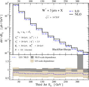
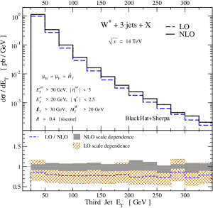
Figure 17: The $E_{T}$ distributions of the third jet, $d\sigma(W\rightarrow e\nu+\geq 3$-jets)$/dE_{T}^{3\rm rd\hbox{-}jet}$, at the LHC. The left panel shows the case of $W^{-}$ and the right of $W^{+}$.

For the inclusive production of $W\,\!+\,3$ jets, a basic quantity to examine is the $E_{T}$ distribution for the thirdmost leading jet in $E_{T}$. This distribution is shown in fig. 17. As in the Tevatron results, the scale uncertainty is considerably reduced at NLO compared to LO. With our default choice of scale $\mu={\hat{H}}_{T}$, the ratio of LO to NLO predictions displayed in the lower panels is rather flat over the entire displayed region. (The upward spike in the NLO band in the $W^{-}$ plot at 300 GeV is due to a statistical fluctuation in the evaluation at $\mu={\hat{H}}_{T}/2$.) This plot may be compared to the $E_{T}$ distribution of the second-most energetic jet shown in the right panel of fig. 9, which undergoes significant shape change between LO and NLO predictions, though less than for the scale choice $\mu=E_{T}^{W}$. The dynamic range we show here is larger than in the corresponding plot for the Tevatron.

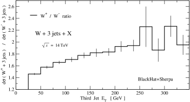
Figure 18: The ratio of the $E_{T}$ distribution of the third jet accompanying a $W^{+}$ to the same distribution for $W^{-}$, evaluated at NLO using $\mu={\hat{H}}_{T}$. The two distributions are shown separately in fig. 17. The thin vertical lines denote the numerical integration errors.

In order to examine shape differences between the $E_{T}$ distributions in $W^{+}$ and $W^{-}$ production, in fig. 18 we show the ratio of the two distributions plotted in fig. 17. The ratio is greater than unity at low $E_{T}$ due to the larger total cross section for $W^{+}$ production compared to $W^{-}$, as given in tables 4 and 5. The ratio increases significantly with $E_{T}$, on the order of 25 percent over the range of the plot, because larger $E_{T}$ forces larger partonic center-of-mass energies, and hence larger values of $x$ where the $u$ quark distribution is more dominant.

The $H_{T}$ distribution also has slightly different shapes for $W^{-}$ and $W^{+}$ production. The right panel of fig. 11 shows the $H_{T}$ distribution in $W^{-}$ production (with $\mu={\hat{H}}_{T}$). The corresponding plot for $W^{+}$ is given in the right panel of fig. 15. Across the displayed range, the ratio of the NLO $W^{+}$ to $W^{-}$ distributions (not shown) increases slightly. The increase occurs for the same reason as the third jet $E_{T}$ distribution.

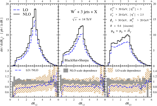
Figure 19: The $\Delta R$ distributions for $W^{-}\,\!+\,3$-jet production, from left to right: between the first and second, first and third, and second and third jets, using the scale choice $\mu={\hat{H}}_{T}$. The $\Delta R_{12}$ distribution between the first and second jets shows a significant shape change in going from LO to NLO, while the other two cases are flat. The distributions for $W^{+}\,\!+\,3$-jet production are similar.

Fig. 19 shows the differential distributions with respect to di-jet separations $\Delta R_{ij}$. The two hardest jets, labeled 1 and 2, are more likely to be produced in a back-to-back fashion, leading to a more peaked distribution around $\pi$. As in other distributions, the NLO scale-dependence band is much smaller than the LO one. The LO and NLO distributions for the separation of the leading two jets are somewhat different from each other in shape. This is presumably due to the effect of additional radiation allowing kinematic configurations where the jets are closer together, thereby pushing the weight of the distribution to smaller $\Delta R$ values, although the position of the peak is essentially unchanged. The shapes of the other two distributions are similar at LO and NLO. All three distributions show sizable shifts in their overall normalization, for $\mu={\hat{H}}_{T}$.

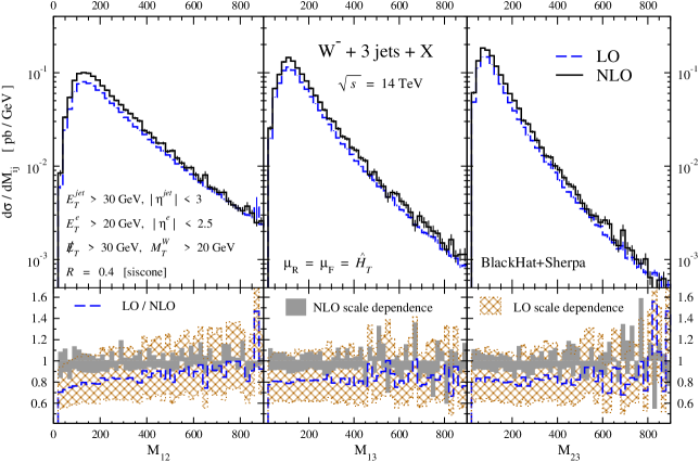
Figure 20: The di-jet masses in $W^{-}+3$-jet production at the LHC; $M_{ij}$ (in GeV) is the invariant mass of the $i$-th and $j$-th leading jets, ordered in $E_{T}$.

Fig. 20 displays distributions for the di-jet masses in $W^{-}\,\!+\,3$-jet production. The three plots in the figure give the di-jet mass of the first and second, first and third, and second and third leading jets, denoted by $M_{ij}$ where $i$ and $j$ label the jets. Although our default choice of scale $\mu={\hat{H}}_{T}$ does significantly reduce the shape changes between LO and NLO compared with the choice $\mu=E_{T}^{W}$ made for the Tevatron (see fig. 7), significant shape changes remain for the $M_{12}$ distribution. For the other two cases the ratio between LO and NLO is rather flat. These features have parallels in the $\Delta R_{ij}$ distributions in fig. 19; the physics of the two leading jets is not modeled especially well at LO.

VI Leptons at the LHC

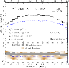
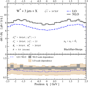
Figure 21: The charged-lepton pseudorapidity distribution at the LHC for $W^{-}$ and $W^{+}$ production.

We now turn from hadronic observables to leptonic ones. At the LHC, the latter distributions depend strongly on whether a $W^{+}$ or a $W^{-}$ boson has been produced.

Fig. 21 shows the pseudorapidity distributions of the daughter charged leptons. Because of the large-$x$ excess of $u$ quarks over $d$ quarks, the $qg$ initial state produces $W^{+}$ preferentially, and tends to produce them more forward; this fact accounts for the larger and more forward positron distribution. The lower panels show that in this case, the NLO corrections modify primarily the overall normalization of these distributions, with only a slight change in shape from LO to NLO.

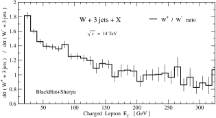
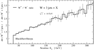
Figure 22: The left panel shows the ratio of the charged-lepton $E_{T}$ distributions at the LHC for $W^{+}$ and $W^{-}$ production, evaluated at NLO, while the right panel shows the corresponding ratio for the neutrino $E_{T}$, or equivalently the missing transverse energy.

In the right panel of fig. 16 we showed the positron transverse momentum distribution in $W^{+}\,\!+\,3$-jet production at the LHC. In order to contrast the distribution with the corresponding distribution in $W^{-}\,\!+\,3$-jet production, fig. 22 shows the ratio of the NLO transverse energy distributions for the $W^{\pm}$ boson decay products, charged leptons in the left panel and neutrinos in the right panel. The plots show dramatic differences between the $W^{+}$ and $W^{-}$ distributions, especially for the neutrino $E_{T}$, or missing transverse energy. The left panel shows a large ratio for $W^{+}$ to $W^{-}$ at small $E_{T}^{e}$ which declines at larger $E_{T}^{e}$. In contrast, the corresponding ratio for the neutrino $E_{T}$, or equivalently the missing transverse energy ${{\raise 0.91666pt\hbox to7.95831pt{\hss/\hss}\hbox to0.0pt{\hss$E$}}}_{T}$ in the event, starts with a somewhat smaller value but increases rapidly with $E_{T}$. This significant increase means that the $W^{+}\,\!+\,n$-jet background to missing-energy-plus-jets signals, when a charged lepton is lost, is more severe than the $W^{-}\,\!+\,n$-jet background by a factor of two to three.

This disparate behavior is presumably due to a net left-handed polarization for high $E_{T}$ $W^{\pm}$ bosons, which is then analyzed by their leptonic decay via the parity-violating charged-current interaction. Before discussing this situation further, it is useful to recall the dynamics underlying the longitudinal (rapidity) charge asymmetry in $W^{\pm}$ production at the Tevatron, and the corresponding asymmetry for the charged lepton into which the $W$ boson decays ESW . At a $p\bar{p}$ collider, the dominance of $u$ quarks over $\bar{d}$ quarks implies that in the process $u\bar{d}\to W^{+}\to e^{+}\nu_{e}$ the $W^{+}$ typically moves in the $u$ quark (proton) direction. Because the charged current is left-handed, the $u$ quark must be left-handed, and the $\bar{d}$ anti-quark right-handed. In order to conserve angular momentum, the $W^{+}$ must be polarized left-handed along its direction of motion, which in this case (at low transverse energy) is preferentially along the beam axis. In the decay $W^{+}\to e^{+}\nu_{e}$, angular-momentum conservation implies that the left-handed $W^{+}$ tends to emit the left-handed neutrino forward, and the right-handed positron backward, relative to its direction of motion. The same arguments show that the $W^{-}$ typically moves in the anti-proton direction, is polarized right-handed, and tends to decay with the left-handed electron backward relative to its direction of motion. Both signs of charged leptons are typically more central than are their parent $W$ bosons. In other words, there is a large asymmetry in the rapidity distribution of $W^{+}$ bosons at the Tevatron, and a strongly diluted asymmetry in the rapidity distribution of the charged decay lepton ESW ; CDFWasym .

Now consider a $pp$ collider (the LHC) and $W^{\pm}$ bosons moving with large momentum primarily transverse to the beam axis, as required to produce the large $E_{T}$ tails for the decay lepton distributions shown in fig. 22. Suppose that both $W^{+}$ and $W^{-}$ bosons are polarized left-handed, with a polarization that increases with $E_{T}^{W}$. Then the $W^{+}$ will tend to emit the left-handed neutrino forward relative to its direction of motion (resulting in a larger transverse energy) and the right-handed positron backward (smaller transverse energy). In contrast, the $W^{-}$ will emit the left-handed electron forward. Such decays will produce an enhancement in the neutrino $E_{T}$ distribution and a depletion in the charged lepton distribution, for $W^{+}$ relative to $W^{-}$, consistent with the ratios displayed in fig. 22. We have checked that the same distributions as shown in fig. 22, but for $W\,\!+\,1,2$-jet production, are very similar. Also, the LO ratios in all cases are virtually indistinguishable from the NLO ones. We examined the LO ratios, removing all lepton acceptance cuts, and the same general trends persist (in fact they are even stronger at moderate lepton $E_{T}$). The left-handed polarization of both $W^{+}$ and $W^{-}$ is also indicated by the corresponding ratios of $W$ transverse momenta (not shown). These ratios grow monotonically with the $W$’s $p_{T}$, but at a lower rate than the ratio for the neutrino $E_{T}$. This growth reflects the fact that the larger the $W$ transverse momentum we require, the larger is the required parton momentum fraction $x$, and thus the more $W^{+}$ is favored over $W^{-}$ by the stiffer $u$ quark distribution.

We do not have a complete understanding of why the $W$ bosons should be polarized left-handed at large transverse momentum, in a manner that is apparently fairly independent of the number of recoiling jets. For $W\,\!+\,1$-jet production at LO, it is possible to examine the relevant helicity amplitudes and make such an argument, based on kinematics and on the dominance of the $qg$ initial state. It is also the case that when a very high transverse-momentum (left-handed) quark splits collinearly to another quark and a $W$ boson, with the $W$ boson taking most of the momentum, the $W$ boson is predominantly left-handed. However, these examples certainly do not exhaust all of the possible polarization mechanisms, and a more thorough explanation would require further study.

VII Jet-Emission Probability at Increased Pseudorapidity Separation

One of the production mechanisms for the Higgs boson at the LHC is via vector-boson fusion VBF , which contains partonic subprocesses such as $qQ\to q^{\prime}Q^{\prime}H$, mediated by the fusion of two $W$ bosons. Because the Higgs is produced via colorless electroweak vector boson exchange, a relative absence of radiation is expected between the two forward tagging quark jets, in comparison with QCD background processes with color exchange. A veto on central jets may play an important role in such searches. For this veto to be effective, the background processes should retain a substantial probability of additional radiation, as the pseudorapidity separation $\Delta\eta$ between two of the jets becomes large. The production of a $W$ boson in association with jets is a prime example of a background-type process dominated by color exchange at LO. In fig. 61 of ref. CHS , a similar question was studied in $W\,\!+\,2$-jet and $W\,\!+\,3$-jet production at the Tevatron, by looking at the probability of finding a third jet in the acceptance as a function of the pseudorapidity separation of the leading two jets, ordered by transverse energy. In that figure, CDF data was compared with a leading-order QCD prediction.

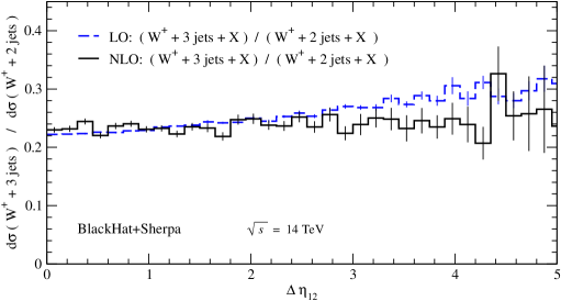
Figure 23: The ratio of the inclusive $W^{+}\,\!+\,3$-jet to $W^{+}\,\!+\,2$-jet cross sections at NLO, as a function of the pseudorapidity separation $\Delta\eta_{12}$ between the leading two jets at the LHC. The solid (black) line gives the NLO result, while the dashed (blue) line represents the LO result. The ratio for $W^{-}$ is very similar, particularly at NLO.

A more appropriate distribution for assessing the effectiveness of a central jet veto would be to order the jets in pseudorapidity, not $E_{T}$, and place an additional constraint that the third jet be between the two most widely-separated jets in pseudorapidity, but here we match the choice made in ref. CHS . In fig. 23 we plot the ratio of the $W^{+}\,\!+\,3$-jet to $W^{+}\,\!+\,2$-jet cross sections at the LHC, as a function of the pseudorapidity separation of the leading two jets, ordered in $E_{T}$. This ratio measures the emission probability of a third jet. The solid line gives the NLO equivalent of the LO Tevatron results in fig. 61 of ref. CHS . As was found at the Tevatron, the emission probability is substantial, over 20%, and remarkably independent of $\Delta\eta_{12}$. Although we plot only the emission probability for jets accompanying a $W^{+}$, the corresponding plot for $W^{-}$ is essentially indistinguishable from it at NLO. (The difference between the LO and NLO results for $W^{-}$ is smaller than the difference shown in fig. 23 for $W^{+}$.)

VIII Subleading-Color Terms

In this section, we turn our attention to the question of simplifying a computation by taking advantage of the structure of color sums. As explained in section II, we can organize the matrix elements—leading-order, real-emission, or virtual—in an expansion in $1/N_{c}$. We expect higher-order terms in this expansion to give smaller contributions numerically; but there are more of them, and their structure is more intricate than that of lower-order terms. In general they take significantly more computer time per event to evaluate. Although one could simply drop these contributions once they have been shown—preferably by direct computation—to be negligible or reliably estimated, we shall describe how to reduce the computer time their direct computation would entail.

In ref. PRLW3BH , we used a particular type of “leading-color” approximation (LC NLO), in which a subset of subleading-color terms were dropped. In the real-emission contributions, as well as in the real-subtraction terms, we retained all terms in the color expansion; the same was also true for the singular terms in the virtual matrix elements. The only approximation was within the finite virtual terms. Here, by “finite” we mean the $\epsilon^{0}$ term in the Laurent expansion of the infrared-divergent one-loop amplitudes in $\epsilon=(4-D)/2$, after extracting a multiplicative factor of $c_{\Gamma}(\epsilon)$ (defined in eq. (25)).

The approximation was defined by first dropping the subleading-color terms, that is those suppressed either by powers of $1/N_{c}^{2}$ (including those coming from leading-color partial amplitudes) or $n_{f}/N_{c}$ (the latter arising from virtual quark loops), in the ratio of the finite virtual terms to the tree-level cross section. In a second step, we multiply this truncated ratio by the tree cross section, with its full color dependence. The net effect of this approximation is to drop quark loops and subleading-color terms in the finite virtual terms that have a different kinematic structure than those at tree level, while retaining the subleading-color terms that have the same kinematic structure. This approximation turns out to be a much better estimate than a strict leading-color approximation (dropping all subleading-color terms in the real-emission terms as well), while still simplifying the calculation considerably by eliminating the need to compute primitive one-loop amplitudes that contribute only to subleading-color terms, such as those shown in fig. 2.

number of jets	CDF	LC NLO	NLO
1	$\;53.5\pm 5.6\;$	$\;58.3(0.1)^{+4.6}_{-4.6}\;$	$\;57.83(0.12)^{+4.36}_{-4.00}\;$
2	$6.8\pm 1.1$	$7.81(0.04)^{+0.54}_{-0.91}$	$7.62(0.04)^{+0.62}_{-0.86}$
3	$0.84\pm 0.24$	$\;0.908(0.005)^{+0.044}_{-0.142}\;$	$0.882(0.005)^{+0.057}_{-0.138}$

Table 8: Comparison of LC NLO to full NLO for the total inclusive cross sections in pb of $W\,\!+\,n$-jet production at the Tevatron using CDF’s cuts WCDF ($E_{T}^{n\rm th\hbox{-}jet}>25$ GeV) and the SISCone algorithm. For reference (see also table 2), the first column gives the CDF data. The second column shows the LC NLO results and the third column the complete NLO results.

Table 8 compares NLO results for the total cross sections at the Tevatron with the experimental setup as in eqs. (17) and (18) except for the tighter jet cut, $E_{T}^{\rm jet}>25\,{\rm GeV}$. For reference, we also show the corresponding CDF data. The column labeled “LC NLO” contains the results computed using the specific leading-color approximation of ref. PRLW3BH . The last column gives the full NLO result, incorporating all subleading-color terms. Previously PRLW3BH , we showed explicitly that this approximation is very good for $W\,\!+\,1,2$-jet production at the Tevatron, leading to errors of no more than three percent. The entry for $W\,\!+\,3$ jets is new, and demonstrates that just as for $W\,\!+\,1$-jet and $W\,\!+\,2$-jet production, the LC approximation is excellent, shifting the total cross section by just under three percent. This shift is much smaller than the NLO scale dependence. In all cases, the LC NLO and complete NLO result are both in excellent agreement with the data.

cut	$\;W^{-}$ LC NLO	$\;W^{-}$ NLO	$\;W^{+}$ LC NLO	$\;W^{+}$ NLO
$\;E_{T}^{\rm jet}>30$ GeV	$\;28.17(0.13)^{+0.99}_{-2.18}\;$	$\;27.52(0.14)^{+1.34}_{-2.81}\;$	$\;42.33(0.27)^{+1.82}_{-2.68}\;$	$\;41.47(0.27)^{+2.81}_{-3.50}$
$\;E_{T}^{\rm jet}>40$ GeV	$14.24(0.07)^{+0.76}_{-1.09}$	$13.96(0.07)^{+1.03}_{-1.31}$	$22.08(0.15)^{+1.20}_{-1.44}$	$21.76(0.15)^{+1.68}_{-1.86}$

Table 9: Comparison of the total cross sections, in pb, between LC NLO and full NLO results for $W\,\!+\,3$-jet prodiction at the LHC with $\sqrt{s}=14$ TeV, using the SISCone algorithm and the cuts of eqs. (21) and (22).

Table 9 shows results for the total cross section of $W\,\!+\,3$-jet production at an LHC energy of 14 TeV, using the cuts given in eqs. (21) and (22). In this case the column labeled “LC NLO” refers to an LC approximation that is slightly modified from the one used for the Tevatron. We avoid rescaling the leading-color virtual contributions by the ratio of the full-color to leading-color cross section; this allows us to simply add together the “leading-color” and remaining “subleading-color” contributions to obtain the total cross section. This modification has only a small effect on the corresponding total cross section. Indeed, for Tevatron cross sections the shift is under 1.5 percent throughout the scale-variation band. (To facilitate comparison to our previously published results PRLW3BH , for Tevatron cross sections we use the identical LC approximation as in that reference.)

The modified LC approximation is again accurate to three percent for central values, and to five percent for the upper or lower edges of the scale-dependence bands. The good quality of the LC approximation also holds for all distributions we have examined. Examples are shown in figs. 24 and 25; for both the Tevatron and the LHC, the corrections due to the subleading-color terms are less than three percent, uniformly across the distributions.

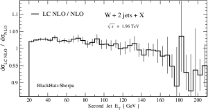
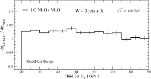
Figure 24: Ratios of our leading-color approximation to a full-color calculation for $E_{T}$ distributions in $W\,\!+\,2,3$-jet production at the Tevatron. The numerical integration errors on each bin are indicated by thin vertical lines. (Different error sources are combined linearly.)

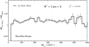
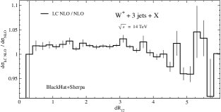
Figure 25: Ratios of our leading-color approximation to a full-color calculation for the leading-dijet invariant mass distribution in $W^{-}\,\!+\,3$-jet production, and for the $\Delta R_{12}$ distribution in $W^{+}\,\!+\,3$-jet production, at the LHC.

The quality of this approximation has important implications for organizing the calculation of virtual contributions. As discussed in section II.2, the primitive amplitudes entering the leading-color approximation used in ref. PRLW3BH and discussed above are a small subset of the primitive amplitudes required for the complete virtual correction. The full result, including subleading-color terms, requires the computation of a much larger number of primitive amplitudes, 336 for two-quark processes and 80 for four-quark processes as opposed to 48 for two-quark processes and 8 for four-quark processes in the leading-color computation. Furthermore, the subleading-color primitive amplitudes shown in fig. 2 have a more complicated analytic structure than the leading-color ones shown in fig. 1, because the $W$ does not have to be ordered with respect to parton(s) emitted between the $W$ boson and the $q$ or $q^{\prime}$. The partial lack of color-ordering implies cuts and poles in more channels. As a result, it takes about 27 times longer per phase-space point to evaluate the subleading-color virtual terms than the leading-color ones.

This large factor may seem to be a cause for concern. However, the smallness of the subleading-color contributions, discussed above, comes to our rescue. If we require that the numerical integration errors due to the subleading-color contributions be comparable to those coming from the leading-color ones, we can allow for larger relative errors in the evaluation of the subleading-color terms. We can adopt a “color-expansion sampling” approach wherein we can use far fewer phase-space points (typically a factor of 20 fewer) to evaluate them NLOZ4Jets as compared to the leading-color terms. (We must ensure that there are sufficient statistics in each bin of every distribution of interest, of course.) There is no need to know ahead of time what the relative size of the two contributions is; we simply stop the integration when the desired numerical precision is reached for each contribution separately. This approach requires only a bit more than a factor of two more computer time for the full-color result than for the leading-color approximation, with our present setup. It saves roughly a factor of thirty in computer time, compared to the naive approach of evaluating the subleading-color terms at every phase-space point. We expect to obtain further improvements in the evaluation efficiency of subleading-color contributions through improved re-use of primitive amplitudes. Together with color-expansion sampling, this should reduce the time required for computing the subleading-color terms to a small fraction of the total computer time. This color-expansion sampling approach would naturally be implemented in a dynamical way by treating the subleading-color contributions as another set of ‘subprocesses’ within the SHERPA multi-channel integration.

Were we seeking to optimize the computer time more aggressively, we would let the total error be dominated by the most time-consuming part of the calculation, namely the subleading-color terms. We have, however, opted for a more conservative approach, keeping the integration error from the subleading-color contributions in line with the errors from the other contributions.

IX Conclusions

In this paper, we presented the first complete NLO study of $W\,\!+\,3$-jet production, incorporating all massless partonic contributions. We compared the total cross section and the third-jet $E_{T}$ distribution to Tevatron data WCDF . We also presented NLO predictions for the $H_{T}$ and di-jet mass distributions. It will be interesting to compare these and other distributions to Tevatron data sets with larger statistics than those already published by CDF WCDF . We presented a variety of distributions at the declared final running energy of the LHC, including many relevant for Standard Model backgrounds to events with large missing energy and to Higgs boson production via vector-boson fusion. As expected, we find a much smaller renormalization- and factorization-scale dependence in all distributions at NLO, compared to LO results. Although the LHC will start running at lower energy, our choice should help facilitate comparisons to earlier studies based on leading-order QCD and matching to parton showers LOPrograms ; HELAC ; Amegic ; Matching ; MLMSMPR ; OtherLOWCodesPartonShowers ; LOComparison .

We have shown explicitly in $W\,\!+\,3$ jet distributions that the scale dependence of LO predictions is not restricted to overall normalizations. An infelicitous choice of scale can change the shapes of distributions substantially between LO and NLO. This effect is much more pronounced at the LHC than at the Tevatron. One can reduce the change in shape of distributions between LO and NLO by choosing a scale dynamically, event by event, corresponding to a typical scale for the event, as noted in, for example, refs. Vplus1NLOAR ; EarlyWplus2MP ; DynamicalScaleChoice . The problem with poor scale choices can be much more severe than just changes in shape between LO and NLO results. Indeed, for sufficiently poor choices, such as the fixed scale $\mu=M_{W}$ or the transverse energy of the $W$ boson, $\mu=E_{T}^{W}$, large logarithms can appear in some distributions, invalidating even an NLO prediction. We find that the total (partonic) transverse energy ${\hat{H}}_{T}$ is a more appropriate scale choice for $W\,\!+\,3$-jet production than the $W$ transverse energy or the fixed scales used in previous Tevatron analyses. (A fixed fraction of the total transverse energy would also be appropriate.) We expect that this scale choice will be appropriate to a variety of higher-multiplicity processes, and recommend its use in LO predictions (when an NLO one is not available) as well as at NLO. A recent paper Bauer motivates a similar type of scale choice using soft-collinear effective theory, and we have contrasted its properties with those of ${\hat{H}}_{T}$. Of course, a simple scale choice is no substitute for a complete NLO prediction. In some distributions, such as the transverse energy of the second-most energetic jet and the $\Delta R$ separation between the two leading jets, the NLO calculation incorporates physics effects that are not captured by simple changes of scale.

We also confirmed that our previous NLO analysis of $W\,\!+\,3$-jet production PRLW3BH , which used a specific leading-color approximation, is valid to within three percent. This error is quite a bit smaller than other uncertainties, such as that implicit in the scale dependence, or that due to uncertainties in the parton distribution functions. However, we can draw this conclusion only after computing the subleading-color terms, as we have done here. To evaluate the subleading-color terms efficiently, we used “color-expansion sampling”. The subleading-color terms require much more computer time per phase space point. However, because they are small, only a few percent of the leading-color ones, we can tolerate a much larger relative error for them from the Monte Carlo integration, thus sampling them much less often. We expect that this general approach will be an effective technique for reducing the computer-time requirements for ever-more complicated processes such as $Z\,\!+\,3$-jet, $W\,\!+\,4$-jet, or $Z\,\!+\,4$-jet production.

In our analyses we mainly used the SISCone jet algorithm; we also presented total cross sections using the $k_{T}$ jet algorithm KTAlgorithm at the LHC. These jet algorithms are infrared-safe to all orders in perturbation theory. With our setup it is a simple matter to replace one infrared-safe cone algorithm with any other desired one. We defer a study of the anti-$k_{T}$ algorithm antikT , which has certain experimental advantages such as uniform catchment areas for soft radiation, to future work. From a perturbative viewpoint, infrared safety is essential; infrared-unsafe quantities are simply logarithmically divergent. In the real world, perturbation theory does not go on forever but is overtaken by non-perturbative dynamics around the confinement scale. Infrared-unsafe quantities are not infinite, but the infinities are cut off and replaced by quantities determined by non-perturbative physics. The logarithms translate SISCONE ; GavinSalamThesis into inverse powers of the strong coupling $\alpha_{S}$, thereby spoiling the perturbative expansion. This is an important practical problem because the jet algorithms traditionally used at the Tevatron by the CDF and D0 collaborations are, in fact, infrared-unsafe beyond the lowest orders SISCONE . Unknown nonperturbative corrections for these algorithms would undo many of the benefits of a higher-order prediction, especially in the context of new, higher statistics data. Accordingly, it is highly desirable that future experimental analyses at both the Tevatron and the LHC use an infrared-safe jet algorithm.

Our paper demonstrates the utility of on-shell methods for computing one-loop matrix elements entering state-of-the-art NLO QCD predictions for processes of phenomenological interest at the LHC. We used BlackHat, an efficient new code library based on these methods. The NLO $W\,\!+\,3$-jet results reported here also demonstrate the functionality of our computational setup, which uses BlackHat in conjunction with the SHERPA package. Besides handling the real-emission contributions and infrared-singular phase space via AMEGIC++, the SHERPA framework offers a convenient set of tools for integrating over phase space and analyzing the results.

There are many relevant processes with large numbers of final-state objects such as jets that remain to be computed, especially those involving vector bosons, jets, heavy quarks and Higgs bosons LesHouches . Such processes are backgrounds to the production of new heavy particles with multi-body decays. Our setup is robust enough to deal systematically with such processes. In the present paper, we have demonstrated the new tools and on-shell methods at work for the non-trivial case of $W\,\!+\,3$-jet production at hadron colliders. We look forward to comparing our predictions against forthcoming LHC data.

Appendix A Squared Matrix Elements at One Point in Phase Space

In order to aid future implementations of virtual corrections for $W\,\!+\,3$-jet production in other numerical codes, we present values of the one-loop virtual corrections to the squared matrix elements, $d\sigma_{V}^{(1)}$, at one point in phase space. This comes from the interference between the tree and one-loop amplitudes, summed over all colors and helicities, for $N_{c}=3$ and $n_{f}=5$ massless quark flavors.

In table 10 we present numerical values for four representative subprocesses. All other subprocesses are related to these four by crossing symmetry. In the second and third lines of table 10, the presence of two identical quarks (after crossing all particles into the final state) means that amplitudes are antisymmetrized under exchange of the two.

$\widehat{d\sigma}_{V}^{(1)}$	$1/\epsilon^{2}$	$1/\epsilon$	$\epsilon^{0}\hskip 27.03003pt$
$(1_{\bar{u}}\,2_{c}\rightarrow 3_{c}\,4_{\bar{d}}\,5_{g}\,6_{e^{-}}7_{\bar{\nu}})$	$-8.333333333$	$-32.37677210$	$1.778061330$
$(1_{\bar{u}}\,2_{u}\rightarrow 3_{u}\,4_{\bar{d}}\,5_{g}\,6_{e^{-}}7_{\bar{\nu}})$	$-8.333333333$	$-32.40807165$	$1.035000256$
$(1_{\bar{u}}\,2_{d}\rightarrow 3_{d}\,4_{\bar{d}}\,5_{g}\,6_{e^{-}}7_{\bar{\nu}})$	$-8.333333333$	$-32.50750136$	$0.4788030624$
$(1_{\bar{u}}\,2_{g}\rightarrow 3_{g}\,4_{g}\,5_{\bar{d}}\,6_{e^{-}}7_{\bar{\nu}})$	$-11.66666667$	$-42.34303628$	$-13.97991225$

Table 10: Numerical values of the normalized virtual correction to the squared matrix elements, $\widehat{d\sigma}_{V}^{(1)}$, at the phase-space point given in the text, for the four basic partonic subprocesses for $W\,\!+\,3$-jet production at a hadron collider. We give the finite parts along with the coefficients of the poles in $\epsilon$.

We quote numerical results for the ultraviolet-renormalized virtual corrections in the ’t Hooft-Veltman variant of dimensional regularization HV . The remaining singularities in the dimensional regularization parameter $\epsilon=(4-D)/2$ arise from the virtual soft and collinear singularities in the one-loop amplitudes.

The quoted values are for the ratio of the virtual corrections to the tree-level squared matrix element $d\sigma^{(0)}$. Explicitly, we define the ratio,

$$\widehat{d\sigma}_{V}^{(1)}\equiv\frac{1}{8\pi\alpha_{S}\,c_{\Gamma}(\epsilon)}\frac{d\sigma_{V}^{(1)}}{d\sigma^{(0)}}\,,$$ (24)

where we have also separated out the dependence on the strong coupling $\alpha_{S}$ and the overall factor $c_{\Gamma}(\epsilon)$, defined by

$$c_{\Gamma}(\epsilon)=\frac{1}{(4\pi)^{2-\epsilon}}\frac{\Gamma(1+\epsilon)\Gamma^{2}(1-\epsilon)}{\Gamma(1-2\epsilon)}\,.$$ (25)

The coupling constants, mass and width of the $W$ boson are given in section II.7. However, the numerical values for the ratio (24), given in table 10, are independent of these parameters; coupling constants as well as the $W$ boson Breit-Wigner factor cancel between the tree and virtual correction terms.

We choose the phase-space point given in eqs. (9.3) and (9.4) of ref. Genhel ,

$$k_{1} = {\mu\over 2}\,(1,-\sin\theta,-\cos\theta\sin\phi,-\cos\theta\cos\phi)\,,$$

$$k_{2} = {\mu\over 2}\,(1,\sin\theta,\cos\theta\sin\phi,\cos\theta\cos\phi)\,,$$

$$k_{3} = {\mu\over 3}(1,1,0,0)\,,$$

$$k_{4} = {\mu\over 8}(1,\cos\beta,\sin\beta,0)\,,$$

$$k_{5} = {\mu\over 10}(1,\cos\alpha\cos\beta,\cos\alpha\sin\beta,\sin\alpha)\,,$$

$$k_{6} = {\mu\over 12}(1,\cos\gamma\cos\beta,\cos\gamma\sin\beta,\sin\gamma)\,,$$

$$k_{7} = k_{1}+k_{2}-k_{3}-k_{4}-k_{5}-k_{6}\,,$$

where

$$\theta={\pi\over 4}\,,\hskip 28.45274pt\phi={\pi\over 6}\,,\hskip 28.45274pt\alpha={\pi\over 3}\,,\hskip 28.45274pt\gamma={2\pi\over 3}\,,\hskip 28.45274pt\cos\beta=-{37\over 128}\,,$$

and the renormalization scale $\mu$ is set to $\mu=7$ GeV. We have flipped the signs of $k_{1}$ and $k_{2}$ compared to ref. Genhel , to correspond to $2\rightarrow 5$ kinematics, instead of $0\rightarrow 7$ kinematics. The labeling of the parton and lepton momenta is indicated explicitly in the first column of Table 10.

References

-
(1)
S. D. Ellis, R. Kleiss and W. J. Stirling,
Phys. Lett. B 158, 341 (1985);
M. L. Mangano, Eur. Phys. J. C 59, 373 (2009) [0809.1567 [hep-ph]]. -
(2)
T. Stelzer and W. F. Long,
Comput. Phys. Commun. 81, 357 (1994)
[hep-ph/9401258];
A. Pukhov et al., hep-ph/9908288;
M. L. Mangano, M. Moretti, F. Piccinini, R. Pittau and A. D. Polosa, JHEP 0307, 001 (2003) [hep-ph/0206293]. -
(3)
A. Kanaki and C. G. Papadopoulos,
Comput. Phys. Commun. 132, 306 (2000)
[hep-ph/0002082];
A. Cafarella, C. G. Papadopoulos and M. Worek, 0710.2427 [hep-ph]. - (4) F. Krauss, R. Kuhn and G. Soff, JHEP 0202, 044 (2002) [hep-ph/0109036].
-
(5)
H. U. Bengtsson and T. Sjöstrand,
Comput. Phys. Commun. 46, 43 (1987);
T. Sjöstrand, P. Eden, C. Friberg, L. Lönnblad, G. Miu, S. Mrenna and E. Norrbin, Comput. Phys. Commun. 135, 238 (2001) [hep-ph/0010017];
G. Marchesini and B. R. Webber, Cavendish-HEP-87/9;
G. Marchesini, B. R. Webber, G. Abbiendi, I. G. Knowles, M. H. Seymour and L. Stanco, Comput. Phys. Commun. 67, 465 (1992);
G. Corcella et al., hep-ph/0210213. - (6) T. Gleisberg, S. Höche, F. Krauss, M. Schönherr, S. Schumann, F. Siegert and J. Winter, JHEP 0902, 007 (2009) [0811.4622 [hep-ph]].
-
(7)
S. Catani, F. Krauss, R. Kuhn and B. R. Webber,
JHEP 0111, 063 (2001)
[hep-ph/0109231];
M. Mangano, presented at the Fermilab ME/MC Tuning Workshop, October 4, 2004. -
(8)
M. L. Mangano, M. Moretti, F. Piccinini and M. Treccani,
JHEP 0701, 013 (2007)
[hep-ph/0611129];
S. Mrenna and P. Richardson, JHEP 0405, 040 (2004) [hep-ph/0312274]. - (9) Z. Bern et al., 0803.0494 [hep-ph].
-
(10)
S. Frixione and B.R. Webber,
JHEP 0206, 029 (2002)
[hep-ph/0204244];
S. Frixione, P. Nason and B.R. Webber, JHEP 0308, 007 (2003) [hep-ph/0305252];
S. Frixione, P. Nason and C. Oleari, JHEP 0711, 070 (2007) [0709.2092 [hep-ph]];
S. Alioli, P. Nason, C. Oleari and E. Re, JHEP 0807, 060 (2008) [0805.4802 [hep-ph]]. -
(11)
H. Fritzsch and P. Minkowski,
Phys. Lett. B 73, 80 (1978);
G. Altarelli, G. Parisi and R. Petronzio, Phys. Lett. B 76, 351 (1978);
K. Kajantie and R. Raitio, Nucl. Phys. B 139, 72 (1978);
K. Kajantie, J. Lindfors and R. Raitio, Nucl. Phys. B 144, 422 (1978). - (12) R. Kleiss and W. J. Stirling, Nucl. Phys. B 262, 235 (1985).
- (13) S. D. Ellis, R. Kleiss and W. J. Stirling, Phys. Lett. B 154, 435 (1985).
- (14) M. L. Mangano and S. J. Parke, Phys. Rev. D 41, 59 (1990).
-
(15)
R. K. Ellis, G. Martinelli and R. Petronzio,
Nucl. Phys. B 211, 106 (1983);
W. T. Giele, E. W. N. Glover and D. A. Kosower, Nucl. Phys. B 403, 633 (1993) [hep-ph/9302225]. - (16) P. B. Arnold and M. H. Reno, Nucl. Phys. B 319, 37 (1989) [Erratum-ibid. B 330, 284 (1990)].
- (17) F. A. Berends, H. Kuijf, B. Tausk and W. T. Giele, Nucl. Phys. B 357, 32 (1991).
-
(18)
F. Abe et al. [CDF Collaboration],
Phys. Rev. Lett. 74, 2626 (1995)
[hep-ex/9503002];
S. Abachi et al. [D0 Collaboration], Phys. Rev. Lett. 74, 2632 (1995) [hep-ex/9503003]. - (19) Z. Bern, L. J. Dixon and D. A. Kosower, Nucl. Phys. B 513, 3 (1998) [hep-ph/9708239].
- (20) Z. Bern, L. J. Dixon, D. C. Dunbar and D. A. Kosower, Nucl. Phys. B 425, 217 (1994) [hep-ph/9403226]; Nucl. Phys. B 435, 59 (1995) [hep-ph/9409265].
-
(21)
E. W. N. Glover and D. J. Miller,
Phys. Lett. B 396, 257 (1997)
[hep-ph/9609474];
Z. Bern, L. J. Dixon, D. A. Kosower and S. Weinzierl, Nucl. Phys. B 489, 3 (1997) [hep-ph/9610370];
J. M. Campbell, E. W. N. Glover and D. J. Miller, Phys. Lett. B 409, 503 (1997) [hep-ph/9706297]. - (22) J. M. Campbell and R. K. Ellis, Phys. Rev. D 65, 113007 (2002) [hep-ph/0202176].
- (23) W. T. Giele, S. Keller and E. Laenen, Phys. Lett. B 372, 141 (1996) [hep-ph/9511449].
- (24) J. M. Campbell, R. K. Ellis, F. Maltoni and S. Willenbrock, Phys. Rev. D 75, 054015 (2007) [hep-ph/0611348].
- (25) F. Febres Cordero, L. Reina and D. Wackeroth, Phys. Rev. D 74, 034007 (2006) [hep-ph/0606102]; Phys. Rev. D 80, 034015 (2009) [0906.1923 [hep-ph]].
- (26) J. M. Campbell, R. K. Ellis, F. Febres Cordero, F. Maltoni, L. Reina, D. Wackeroth and S. Willenbrock, Phys. Rev. D 79, 034023 (2009) [0809.3003 [hep-ph]].
- (27) Z. Bern, L. J. Dixon and D. A. Kosower, Annals Phys. 322, 1587 (2007) [0704.2798 [hep-ph]].
- (28) A. Bredenstein, A. Denner, S. Dittmaier and S. Pozzorini, JHEP 0808, 108 (2008) [0807.1248 [hep-ph]]; Phys. Rev. Lett. 103, 012002 (2009) [0905.0110 [hep-ph]].
- (29) G. Ossola, C. G. Papadopoulos and R. Pittau, JHEP 0803, 042 (2008) [0711.3596 [hep-ph]].
- (30) C. F. Berger, Z. Bern, L. J. Dixon, F. Febres Cordero, D. Forde, H. Ita, D. A. Kosower and D. Maître, Phys. Rev. D 78, 036003 (2008) [0803.4180 [hep-ph]].
- (31) W. T. Giele and G. Zanderighi, JHEP 0806, 038 (2008) [0805.2152 [hep-ph]].
-
(32)
A. Lazopoulos,
0812.2998 [hep-ph];
J. C. Winter and W. T. Giele, 0902.0094 [hep-ph]. - (33) A. van Hameren, C. G. Papadopoulos and R. Pittau, 0903.4665 [hep-ph].
- (34) C. F. Berger et al., Phys. Rev. Lett. 102, 222001 (2009) [0902.2760 [hep-ph]].
- (35) T. Aaltonen et al. [CDF Collaboration], Phys. Rev. D 77, 011108 (2008) [0711.4044 [hep-ex]].
- (36) F. Abe et al. [CDF Collaboration], Phys. Rev. Lett. 75, 3997 (1995) [hep-ex/9506006].
- (37) G. P. Salam and G. Soyez, JHEP 0705, 086 (2007) [0704.0292 [hep-ph]].
-
(38)
S. Frixione,
Nucl. Phys. B 410, 280 (1993);
U. Baur, T. Han and J. Ohnemus, Phys. Rev. D 53, 1098 (1996) [hep-ph/9507336]; Phys. Rev. D 57, 2823 (1998) [hep-ph/9710416];
L. J. Dixon, Z. Kunszt and A. Signer, Phys. Rev. D 60, 114037 (1999) [hep-ph/9907305];
G. Bozzi, B. Jäger, C. Oleari and D. Zeppenfeld, Phys. Rev. D 75, 073004 (2007) [hep-ph/0701105]. -
(39)
F. Abe et al. [CDF Collaboration],
Phys. Rev. Lett. 77, 448 (1996)
[hep-ex/9603003];
T. Aaltonen et al. [CDF - Run II Collaboration], Phys. Rev. Lett. 100, 102001 (2008) [0711.3717 [hep-ex]]. - (40) C. W. Bauer and B. O. Lange, 0905.4739 [hep-ph].
- (41) R. K. Ellis, K. Melnikov and G. Zanderighi, JHEP 0904, 077 (2009) [0901.4101 [hep-ph]].
- (42) R. K. Ellis, K. Melnikov and G. Zanderighi, 0906.1445 [hep-ph].
- (43) R. K. Ellis, W. T. Giele, Z. Kunszt and K. Melnikov, 0806.3467 [hep-ph].
- (44) W. T. Giele, Z. Kunszt and K. Melnikov, JHEP 0804, 049 (2008) [0801.2237 [hep-ph]].
- (45) C. F. Berger, Z. Bern, L .J. Dixon, F. Febres Cordero, D. Forde, H. Ita, D. A. Kosower and D. Maître, 0808.0941 [hep-ph].
- (46) S. Catani and M. H. Seymour, Phys. Lett. B 378, 287 (1996) [hep-ph/9602277]; Nucl. Phys. B 485, 291 (1997) [Erratum-ibid. B 510, 503 (1998)] [hep-ph/9605323].
- (47) T. Gleisberg and F. Krauss, Eur. Phys. J. C 53, 501 (2008) [0709.2881 [hep-ph]].
-
(48)
M. H. Seymour and C. Tevlin,
0803.2231 [hep-ph];
K. Hasegawa, S. Moch and P. Uwer, Nucl. Phys. Proc. Suppl. 183, 268 (2008) [0807.3701 [hep-ph]];
R. Frederix, T. Gehrmann and N. Greiner, JHEP 0809, 122 (2008) [0808.2128 [hep-ph]];
M. Czakon, C. G. Papadopoulos and M. Worek, JHEP 0908, 085 (2009) [0905.0883 [hep-ph]]. - (49) L. J. Dixon and A. Signer, Phys. Rev. D 56, 4031 (1997) [hep-ph/9706285].
- (50) R. Kleiss and R. Pittau, Comput. Phys. Commun. 83, 141 (1994) [hep-ph/9405257].
- (51) Z. Bern, L. J. Dixon and D. A. Kosower, Nucl. Phys. B 437, 259 (1995) [hep-ph/9409393].
-
(52)
R. Britto, F. Cachazo and B. Feng,
Nucl. Phys. B 715, 499 (2005)
[hep-th/0412308];
R. Britto, F. Cachazo, B. Feng and E. Witten, Phys. Rev. Lett. 94, 181602 (2005) [hep-th/0501052]. -
(53)
Z. Bern, L. J. Dixon and D. A. Kosower,
Phys. Rev. D 71, 105013 (2005)
[hep-th/0501240];
Phys. Rev. D 72, 125003 (2005)
[hep-ph/0505055];
Phys. Rev. D 73, 065013 (2006)
[hep-ph/0507005];
D. Forde and D. A. Kosower, Phys. Rev. D 73, 065007 (2006) [hep-th/0507292]; Phys. Rev. D 73, 061701 (2006) [hep-ph/0509358];
C. F. Berger, Z. Bern, L. J. Dixon, D. Forde and D. A. Kosower, Phys. Rev. D 75, 016006 (2007) [hep-ph/0607014]. - (54) R. Britto, F. Cachazo and B. Feng, Nucl. Phys. B 725, 275 (2005) [hep-th/0412103].
- (55) G. Ossola, C. G. Papadopoulos and R. Pittau, Nucl. Phys. B 763, 147 (2007) [hep-ph/0609007].
- (56) R. K. Ellis, W. T. Giele and Z. Kunszt, JHEP 0803, 003 (2008) [0708.2398 [hep-ph]].
- (57) D. Forde, Phys. Rev. D 75, 125019 (2007) [0704.1835 [hep-ph]].
- (58) R. J. Eden, P. V. Landshoff, D. I. Olive and J. C. Polkinghorne, The Analytic S Matrix (Cambridge University Press, 1966).
-
(59)
W. T. Giele and E. W. N. Glover,
JHEP 0404, 029 (2004)
[hep-ph/0402152];
T. Binoth, J. P. Guillet, G. Heinrich, E. Pilon and C. Schubert, JHEP 0510, 015 (2005) [hep-ph/0504267];
A. Denner and S. Dittmaier, Nucl. Phys. B 734, 62 (2006) [hep-ph/0509141]. T. Binoth, J. P. Guillet, G. Heinrich, E. Pilon and T. Reiter, 0810.0992 [hep-ph]. - (60) T. Binoth et al., 0807.0605 [hep-ph].
- (61) C. F. Berger, Z. Bern, L. J. Dixon, D. Forde and D. A. Kosower, Phys. Rev. D 74, 036009 (2006) [hep-ph/0604195].
- (62) Z. Bern, L. J. Dixon and D. A. Kosower, Ann. Rev. Nucl. Part. Sci. 46, 109 (1996) [hep-ph/9602280].
-
(63)
L. M. Brown and R. P. Feynman,
Phys. Rev. 85, 231 (1952);
L.M. Brown, Nuovo Cim. 21, 3878 (1961);
B. Petersson, J. Math. Phys. 6, 1955 (1965);
G. Källén and J.S. Toll, J. Math. Phys. 6, 299 (1965);
D. B. Melrose, Nuovo Cim. 40, 181 (1965);
G. Passarino and M. J. G. Veltman, Nucl. Phys. B 160, 151 (1979);
W. L. van Neerven and J. A. M. Vermaseren, Phys. Lett. B 137, 241 (1984);
Z. Bern, L. J. Dixon and D. A. Kosower, Phys. Lett. B 302, 299 (1993) [Erratum-ibid. B 318, 649 (1993)] [hep-ph/9212308];
J. Fleischer, F. Jegerlehner and O. V. Tarasov, Nucl. Phys. B 566, 423 (2000) [hep-ph/9907327];
T. Binoth, J. P. Guillet and G. Heinrich, Nucl. Phys. B 572, 361 (2000) [hep-ph/9911342];
G. Duplanc̆ić and B. Niz̆ić, Eur. Phys. J. C 35, 105 (2004) [hep-ph/0303184]. -
(64)
G. ’t Hooft and M. J. G. Veltman,
Nucl. Phys. B 153, 365 (1979);
G. J. van Oldenborgh and J. A. M. Vermaseren, Z. Phys. C 46, 425 (1990);
W. Beenakker and A. Denner, Nucl. Phys. B 338, 349 (1990);
A. Denner, U. Nierste and R. Scharf, Nucl. Phys. B 367, 637 (1991);
Z. Bern, L. J. Dixon and D. A. Kosower, Nucl. Phys. B 412 (1994) 751 [hep-ph/9306240];
T. Hahn and M. Pérez-Victoria, Comput. Phys. Commun. 118, 153 (1999) [hep-ph/9807565];
R. K. Ellis and G. Zanderighi, JHEP 0802, 002 (2008) [0712.1851 [hep-ph]]. -
(65)
F. A. Berends, R. Kleiss, P. De Causmaecker, R. Gastmans and T. T. Wu,
Phys. Lett. B 103, 124 (1981);
P. De Causmaecker, R. Gastmans, W. Troost and T. T. Wu, Nucl. Phys. B 206, 53 (1982);
Z. Xu, D. H. Zhang and L. Chang, TUTP-84/3-TSINGHUA;
J. F. Gunion and Z. Kunszt, Phys. Lett. B 161, 333 (1985);
Z. Xu, D. H. Zhang and L. Chang, Nucl. Phys. B 291, 392 (1987). - (66) E. Witten, Commun. Math. Phys. 252, 189 (2004) [hep-th/0312171].
-
(67)
Z. Bern and A. G. Morgan,
Nucl. Phys. B 467, 479 (1996)
[hep-ph/9511336];
Z. Bern, L. J. Dixon, D. C. Dunbar and D. A. Kosower, Phys. Lett. B 394, 105 (1997) [hep-th/9611127]. -
(68)
C. Anastasiou, R. Britto, B. Feng, Z. Kunszt and P. Mastrolia,
Phys. Lett. B 645, 213 (2007)
[hep-ph/0609191];
R. Britto and B. Feng, JHEP 0802, 095 (2008) [0711.4284 [hep-ph]]. - (69) G. Ossola, C. G. Papadopoulos and R. Pittau, JHEP 0805, 004 (2008) [0802.1876 [hep-ph]].
- (70) W. L. van Neerven, Nucl. Phys. B 268, 453 (1986).
- (71) R. K. Ellis, W. T. Giele, Z. Kunszt, K. Melnikov and G. Zanderighi, JHEP 0901, 012 (2009) [0810.2762 [hep-ph]].
- (72) S. D. Badger, JHEP 0901, 049 (2009) [0806.4600 [hep-ph]].
-
(73)
M. L. Mangano and S. J. Parke,
Phys. Rept. 200, 301 (1991);
L. J. Dixon, in QCD & Beyond: Proceedings of TASI ’95, ed. D. E. Soper (World Scientific, 1996) [hep-ph/9601359]. -
(74)
W. B. Kilgore,
0711.5015 [hep-ph];
R. Britto, B. Feng and P. Mastrolia, Phys. Rev. D 78, 025031 (2008) [0803.1989 [hep-ph]];
S. D. Badger, Nucl. Phys. Proc. Suppl. 183, 220 (2008) [0807.1245 [hep-ph]];
R. Britto and B. Feng, 0904.2766 [hep-th]. - (75) Y. Hida, X. S. Li and D. H. Bailey, http://crd.lbl.gov/~dhbailey/mpdist, report LBNL-46996.
- (76) M. Seymour, private communication.
- (77) Z. Nagy, Phys. Rev. D 68, 094002 (2003) [hep-ph/0307268].
- (78) G. P. Lepage, J. Comput. Phys. 27, 192 (1978).
- (79) J. Pumplin et al., JHEP 0207, 012 (2002) [hep-ph/0201195].
-
(80)
W. T. Giele and E. W. N. Glover,
Phys. Rev. D 46 (1992) 1980;
Z. Kunszt, A. Signer and Z. Trócsányi, Nucl. Phys. B 420 (1994) 550 [hep-ph/9401294]. - (81) B. D. Cooper, PhD thesis, FERMILAB-THESIS-2006-61.
- (82) F. Abe et al. [CDF Collaboration], Phys. Rev. D 45, 1448 (1992).
-
(83)
R. Akers et al. [OPAL Collaboration],
Z. Phys. C 63, 197 (1994);
M. H. Seymour, Nucl. Phys. B 513, 269 (1998) [hep-ph/9707338]. -
(84)
S. Höche, F. Krauss, N. Lavesson, L. Lönnblad, M. Mangano,
A. Schälicke and S. Schumann,
hep-ph/0602031;
J. Alwall et al., Eur. Phys. J. C 53, 473 (2008) [0706.2569 [hep-ph]]. - (85) D. Stump, J. Huston, J. Pumplin, W. K. Tung, H. L. Lai, S. Kuhlmann and J. F. Owens, JHEP 0310, 046 (2003) [hep-ph/0303013].
- (86) J. M. Campbell, J. W. Huston and W. J. Stirling, Rept. Prog. Phys. 70, 89 (2007) [hep-ph/0611148].
-
(87)
S. Catani, Y. L. Dokshitzer, M. H. Seymour and B. R. Webber,
Nucl. Phys. B 406, 187 (1993);
S. D. Ellis and D. E. Soper, Phys. Rev. D 48, 3160 (1993) [hep-ph/9305266]. - (88) R. K. Ellis, W. J. Stirling and B.R. Webber, QCD and Collider Physics (Cambridge University Press, 1996).
- (89) T. Aaltonen et al. [CDF Collaboration], Phys. Rev. Lett. 102, 181801 (2009) [0901.2169 [hep-ex]].
-
(90)
D. Zeppenfeld, R. Kinnunen, A. Nikitenko and E. Richter-Was,
Phys. Rev. D 62, 013009 (2000)
[hep-ph/0002036];
M. Dührssen, S. Heinemeyer, H. Logan, D. Rainwater, G. Weiglein and D. Zeppenfeld, Phys. Rev. D 70, 113009 (2004) [hep-ph/0406323]. -
(91)
F. Krauss, A. Schälicke, S. Schumann and G. Soff,
Phys. Rev. D 70, 114009 (2004)
[hep-ph/0409106];
Phys. Rev. D 72, 054017 (2005)
[hep-ph/0503280];
N. Lavesson and L. Lönnblad, JHEP 0507, 054 (2005) [hep-ph/0503293]. - (92) M. Cacciari, G. P. Salam and G. Soyez, JHEP 0804, 063 (2008) [0802.1189 [hep-ph]].
- (93) G. P. Salam, 0906.1833 [hep-ph].
- (94) G. ’t Hooft and M. Veltman, Nucl. Phys. B 44, 189 (1972).