Density profiles and density oscillations of an interacting three-component normal Fermi gas

Abstract

We use a semiclassical approximation to investigate density variations and dipole oscillations of an interacting three-component normal Fermi gas in a harmonic trap. We consider both attractive and repulsive interactions between different pairs of fermions and study the effect of population imbalance on densities. We find that the density profiles significantly deviate from those of non-interacting profiles and extremely sensitive to interactions and population imbalance. Unlike for a two-component Fermi system, we find density imbalance even for balanced populations. For some range of parameters, one component completely repels from the trap center giving rise a donut shape density profile. Further, we find that the in-phase dipole oscillation frequency is consistent with Kohn’s theorem and other two dipole mode frequencies are strongly effected by the interactions and the number of atoms in the harmonic trap.

I I. Introduction

The recent experimental progress of trapping and cooling of atomic gases leads to an opportunity for a detail study of exciting many body physics ex . The key to this exciting opportunity is that the high experimental controllability of these systems. For a dilute atomic mixture, the quantum degenerate regime can be achieved by cooling the system to ultra-cold temperatures. In these ultra-cold atomic systems, one of the fascinating control parameters has been the two-body scattering length of atoms. Tuning the scattering length, simply by applying a homogenous magnetic field (Feshbach resonance fb ), the interactions can be controlled dramatically. The fundamental differences between fermions and bosons take place in the quantum degenerate regime. For the case of two-component Fermi systems, if the temperature is low enough, weakly bound molecules could be formed at positive scattering lengths and these molecules can undergo Bose-Einstein condensation. By sweeping the magnetic field, the scattering length can be further increased to a divergency and can be changed in sign. In this strongly interacting limit, the bosonic molecules continuously transform into Bardeen, Cooper and Schrieffer (BCS) superfluid pairs. The physics of this so-called BCS-BEC crossover region is relevant to the systems like high $T_{C}$ superconductors, superfluid ³He, and neutron stars. The recent realization of three-component degenerate Fermi gases has opened a new research frontier in ultra-cold atoms. These three-component systems have relevance to high density quark matter, neutron stars, and universal few body physics. Therefore, superfluid phases and phase separation in a three-component Fermi gas can be treated as an analogous to color superconductivity and baryon formation in quantum chromo dynamics.

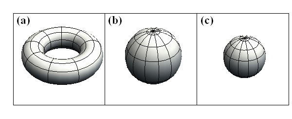
Figure 1: Schematic atomic cloud shapes of a population imbalanced three-component Fermi gas in a spherically symmetric harmonic trap. Depending on the interaction between different pairs of fermions and the population imbalance, one component can completely repel from the trap center as shown in panel (a). The other two components form a spherical shape as shown in panels (b) and (c). See FIG. 4 for quantitative details. For a population balance mixture, inner radius of the donut shape cloud is zero and we find density imbalance through out the harmonic trap.

In a recent experiment by Bartenstein et al grimm , using radio frequency spectroscopic data, molecular binding energies, scattering lengths and the Feshbach resonance positions of the lowest three channels of ⁶Li atoms have been determined. As there are three broad s-wave Feshbach resonances for the three lowest hyperfine states of ⁶Li system, one can prepare the system at various atomic interactions between different pairs. In another recent experimental development by Ottenstein et al jochim , a three-component Fermi gas has been cooled down to the quantum degenerate regime. In this experiment, the three lowest hyperfine states of ⁶Li atoms are prepared at a temperature $T=0.37T_{F}$, where $T_{F}$ is the Fermi temperature. During the experiment, the scattering lengths for the respective three Feshbach channels are varied by sweeping a magnetic field and collisional stability of the lowest three channels of ⁶Li atoms has been studied. The most recent experiment ohara reports the first measurements of three-body loss coefficients for a three-component Fermi gas at temperature $T=0.59T_{F}$. By further lowering the temperature, paring of three components can be activated. This promising experimental observations of three-component superfluidity is yet to be realized in near future. Motivated by the realization of these normal degenerate three-component Fermi systems grimm ; jochim ; ohara ; jochimA , we study the ground state normal density profiles and dipole density oscillations of a three-component Fermi gas trapped in a harmonic potential at zero temperature. We use a semiclassical theory known as Thomas Fermi functional approach to investigate the normal state density profiles and dipole density oscillations. In general, at high enough temperatures, the particles are classical so that the semiclassical approximation is valid. In the present paper, we are considering a large number of Fermi atoms. These atoms fill every energy levels up to the Fermi energy $E_{F}$ and $E_{F}$ is larger than the ground state energy. Therefore, a three-component normal Fermi gas can be well described in the semiclassical approximation even at very low temperatures provided that the number of atoms present in the system is large.

For an equal population system, we find that the density imbalanced cloud form a three-shell structure. Depending on the interactions between pairs, density of the one component shows non -monotonic behavior as the cloud extends from center to the edge of the harmonic trap. For an unequal population system, we find very similar behavior as the population balanced system, however, one component completely repels from the trap center. This repulsion depends on both interaction and the population imbalance. The generic shapes of the atomic clouds in a harmonic trapping potential for this case are schematically shown in FIG. 1. In the presence of harmonic trapping potential, we derive expressions for in-phase and and out-of-phase dipole oscillation frequencies as functions of interactions and atom numbers in different spin states. we find that the in-phase oscillation frequency is independent of the interactions and the atom numbers while the out-of-phase oscillation frequencies strongly depend on them.

The paper is organized as follows. In the following section, we present the basic formalism required for the densities and dipole oscillation frequencies. In section III, we derive the equations for Thomas Fermi density profiles and stability condition and then present our self consistent solutions based phase diagram and the density profiles. In section IV, we present dipole oscillation frequencies as a function of interactions and atom numbers followed by the discussions and summary in section V.

II II. Basic Formalism

We assume that the three-component Fermi gas is trapped in a harmonic potential given by $V(r)=(\omega_{\perp}r_{1}^{2}+\omega_{\perp}r_{2}^{2}+\omega_{z}r_{3}^{2})/(2m)$, where $\omega_{\perp}$, $\omega_{z}$, and $m$ are transverse and axial trapping frequencies and mass of an atom respectively. Here $r_{i}$ is the $i$th cartesian component of the position vector $\vec{r}$. Let us denote the density of the $\sigma$ component is $n_{\sigma}$ and the interaction strength between $\sigma$ and $\nu$ components is $U_{\sigma\nu}$.

As we are considering a dilute atomic system at zero temperature, and the interactions are short-range in nature, s-wave scattering channel is dominated over the other scattering channels. Therefore, we can neglect the higher wave scatterings and the interaction can be specified by a single parameter $a_{\sigma\nu}$, which is the s-wave scattering length between component $\sigma$ and $\nu$. The functional form of the interaction is $U_{\sigma\nu}=4\pi\hbar^{2}a_{\sigma\nu}/m$. In order to derive the ground state densities of the normal state at zero temperature, we write the grand canonical energy as a functional of densities, $E_{0}=E_{g}-\sum_{\sigma=1}^{3}\mu_{\sigma}N_{\sigma}$. Here the number of atoms in each spin state $N_{\sigma}=\int d^{3}\vec{r}n_{\sigma}$ and the total energy $E_{g}=\int\epsilon d^{3}\vec{r}$, where $\epsilon$ is given by

$$\epsilon=\sum_{\sigma=1}^{3}\biggr{\{}\frac{\hbar^{2}A}{2m}n_{\sigma}^{5/3}+V(r)n_{\sigma}\biggr{\}}+$$

$$\frac{4\pi\hbar^{2}}{m}\biggr{\{}a_{23}n_{2}n_{3}+a_{13}n_{1}n_{3}+a_{12}n_{1}n_{2}\biggr{\}},$$ (1)

and $A\equiv(3/5)(6\pi^{2})^{2/3}$. Notice we introduced three Lagrange multipliers $\mu_{\sigma}$ (chemical potentials) to constrain the number of atoms in each $\sigma$ state. In section III presented below, we derive Thomas-Fermi equations for the densities from the variation of the total energy.

In the presence of harmonic trapping potential, the lowest lying collective excitations are the dipole or the center of mass oscillations. By generalizing the scaling method used in Ref. 2comptf3 , we derive expressions for the dipole oscillation frequencies for a three-component system. We assume that the atomic cloud is displaced linearly along $r_{3}$ direction. The time varying density of the $\sigma$ component is parameterized by the collective coordinate $\eta_{\sigma}(t)$ as $n_{\sigma}(r,t)=n^{(0)}_{\sigma}(r_{1},r_{2},r_{3}-\eta_{\sigma})$, where $n^{(0)}_{\sigma}(r)$ is the ground state equilibrium density distribution of the $\sigma$ component. Substituting $n_{\sigma}(r,t)$ into total energy expression, the variation of the total energy up to the quadratic order in $\mathbf{\eta}$ is given by

$$\Delta E=E-E_{0}\approx-\frac{1}{2}m\omega^{2}_{z}\sum_{\sigma}\eta_{\sigma}^{2}N_{\sigma}$$

$$+A_{12}(2\eta_{1}\eta_{2}-\eta^{2}_{1}-\eta_{2}^{2})$$

$$+A_{13}(2\eta_{1}\eta_{3}-\eta^{2}_{1}-\eta_{3}^{2})$$

$$+A_{23}(2\eta_{2}\eta_{3}-\eta^{2}_{2}-\eta_{3}^{2})$$ (2)

where

$$A_{\sigma\nu}=\frac{U_{\sigma\nu}}{2}\int d^{3}\vec{r}\frac{\partial n^{(0)}_{\sigma}}{\partial r_{3}}\frac{\partial n^{(0)}_{\nu}}{\partial r_{3}}.$$ (3)

The dipole oscillation frequencies ($\omega_{d}$) are determined by the eigenvalues of the classical equations of motion for $\mathbf{\eta}$. The classical equation of motion in the matrix form is given as,

$$\left(\begin{array}[]{ccc}m(\omega_{z}^{2}-\omega_{d}^{2})N_{1}-2A_{12}-2A_{13}&2A_{12}&2A_{13}\\ 2A_{12}&m(\omega_{z}^{2}-\omega_{d}^{2})N_{2}-2A_{12}-2A_{23}&2A_{23}\\ 2A_{13}&2A_{23}&m(\omega_{z}^{2}-\omega_{d}^{2})N_{3}-2A_{13}-2A_{23}\\ \end{array}\right)\left(\begin{array}[]{c}\eta_{1}\\ \eta_{2}\\ \eta_{3}\\ \end{array}\right)=0.$$ (10)

III III. Thomas-Fermi equations for densities

Before we derive the Thomas-Fermi equations, we introduce three dimensionless variables; $\rho_{\sigma}\equiv n_{\sigma}\zeta^{3}$, $\tilde{r}^{2}\equiv\tilde{r}_{1}^{2}+\tilde{r}_{2}^{2}+\tilde{r}_{3}^{2}$ and $\tilde{a}_{\sigma\nu}\equiv(4\pi)^{2}a_{\sigma\nu}/\zeta$ where $\zeta=\sqrt{\hbar/m\omega}$ is the effective oscillator length with $\omega=(\omega_{\perp}^{2}\omega_{z})^{1/3}$. The dimensionless cartesian component of the vector $\vec{r}$ are defined as $\tilde{r}_{i}\equiv[2\pi m/(\hbar\omega)\omega_{i}^{2}]^{1/2}r_{i}$. In terms of dimensionless variables, now the trapping potential has a symmetric form given by $V(r)=\hbar\omega\tilde{r}^{2}/(4\pi)$. In terms of dimensionless parameters, the number equation and the total energy are given by

$$N_{\sigma}=4\pi\int\tilde{r}^{2}\rho_{\sigma}d\tilde{r},$$ (11)

and

$$\frac{E}{\hbar\omega}=\int\tilde{r}^{2}d\tilde{r}\biggr{\{}\sum_{\sigma=1}^{3}\biggr{(}2\pi A\rho_{\sigma}^{5/3}+\tilde{r}^{2}\rho_{\sigma}-\tilde{\mu}_{\sigma}\rho_{\sigma}\biggr{)}$$

$$+\tilde{a}_{23}\rho_{2}\rho_{3}+\tilde{a}_{13}\rho_{1}\rho_{3}+\tilde{a}_{12}\rho_{1}\rho_{2}\biggr{\}}.$$ (12)

where the dimensionless chemical potential $\tilde{\mu}_{\sigma}=4\pi\mu_{\sigma}/(\hbar\omega)$. The Thomas-Fermi equations for the densities $\rho_{\sigma}$ are derived from the variation of the total energy; $\partial E/\partial\rho_{\sigma}=0$.

$$\frac{10\pi A\rho_{1}^{\frac{2}{3}}}{3}+\tilde{a}_{13}\rho_{3}+\tilde{a}_{12}\rho_{2}=\tilde{\mu}_{1}-\tilde{r}^{2}$$

$$\frac{10\pi A\rho_{2}^{\frac{2}{3}}}{3}+\tilde{a}_{23}\rho_{3}+\tilde{a}_{12}\rho_{1}=\tilde{\mu}_{2}-\tilde{r}^{2}$$

$$\frac{10\pi A\rho_{3}^{\frac{2}{3}}}{3}+\tilde{a}_{23}\rho_{2}+\tilde{a}_{13}\rho_{1}=\tilde{\mu}_{3}-\tilde{r}^{2}$$ (13)

For the spatial density variations, these equations must be solved with the stability condition. The stability condition can be derived from the determinant of second order variation of the energy functional, $|\partial^{2}E/\partial\rho_{\sigma}\partial\rho_{\nu}|\geq 0$, where $\partial^{2}E/\partial\rho_{\sigma}\partial\rho_{\nu}$ is a $3\times 3$ matrix. In terms of dimensionless variables, this stability condition reads,

$$\frac{2}{3}\biggr{(}\frac{10\pi A}{3}\biggr{)}(\tilde{a}_{23}^{2}\rho_{2}^{\frac{1}{3}}\rho_{3}^{\frac{1}{3}}+\tilde{a}_{13}^{2}\rho_{1}^{\frac{1}{3}}\rho_{3}^{\frac{1}{3}}+\tilde{a}_{12}^{2}\rho_{1}^{\frac{1}{3}}\rho_{2}^{\frac{1}{3}})$$

$$-2\tilde{a}_{12}\tilde{a}_{23}\tilde{a}_{13}\rho_{1}^{\frac{1}{3}}\rho_{2}^{\frac{1}{3}}\rho_{3}^{\frac{1}{3}}\leq\biggr{(}\frac{2}{3}\frac{10\pi A}{3}\biggr{)}^{3}$$ (14)

Similar set of equations for an repulsively interacting two-component normal gas in three dimensions are derived in Refs. 2comptf1 ; 2comptf2 ; 2comptf3 . For a two-component normal gas in two dimensions, the Thomas Fermi equations are derived in Ref. 2comptf2D . We have investigated the stability condition given in Eq. (III). Unlike two-component Fermi gases, three-component Fermi mixtures are stable for large densities and interactions jochim . For a dilute system, we do not expect three body collisions to take place so that the system will be stable for a wide range of interactions.

Before we investigate the density variations, let us construct the phase diagram for a homogenous system. We consider a set of representative parameters by fixing the dimensionless chemical potentials of components one and two as $\tilde{\mu}_{1}=190$ and $\tilde{\mu}_{2}=178$ (these values are corresponding to the central chemical potentials of the system with particle numbers in the order of $10^{5}$). Further, we chose the interactions to be $\tilde{a}_{23}=2.5$ and $\tilde{a}_{13}=3.6$. Then by solving the equations (III) and (III), the phase diagram is constructed in $\tilde{a}_{12}$ - $(\tilde{\mu}_{3}-\tilde{\mu}_{2})$ parameter space as shown in FIG. 2. When there is no interaction between component one and two ($a_{12}=0$), the phase boundaries can be easily evaluated analytically. Let us define the possible phases by the notation $i=$ I, II, and III, where $i$ is the phase with component $i$. The mixed phases are defined as sum of $i$’s (For example, I+II is the phase where both component one and two exist). The phase boundary between I+II and I+II+III phases is given by $\tilde{\mu}_{3}=\beta_{23}\tilde{\mu}_{2}^{3/2}+\beta_{13}\tilde{\mu}_{1}^{3/2}$, where $\beta_{\sigma\nu}=3\tilde{a}_{\sigma\nu}/(10\pi A)$. The boundary between I+II+III and II+III phases is given by $\tilde{\mu}_{3}=(\tilde{\mu}_{1}/\beta_{13})^{2/3}+\sqrt{\tilde{\mu}_{2}-\tilde{\mu}_{1}\beta_{23}/\beta_{13}}(\tilde{\mu}_{2}\beta_{23}-\tilde{\mu}_{1}\beta^{2}_{23}/\beta_{13})$. The phase boundary between II + III and III phases is given by $\tilde{\mu}_{3}=(\tilde{\mu}_{2}/\beta_{23})^{2/3}$. Even though, we have restricted ourselves to the repulsive interactions between two-three and one-three pairs, one can consider attractive interactions between these pairs and construct the phase diagram in similar manner.

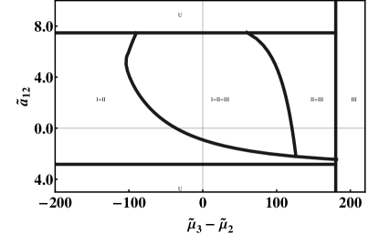
Figure 2: Phase diagram for fixed $\mu_{1}=(4\pi/\hbar\omega)190$, $\mu_{2}=(4\pi/\hbar\omega)178$, $\tilde{a}_{23}=2.5$, and $\tilde{a}_{13}=3.6$. The labels I, II, and III are the phases with component one, two, and three respectively. Label U denotes the unstable region.

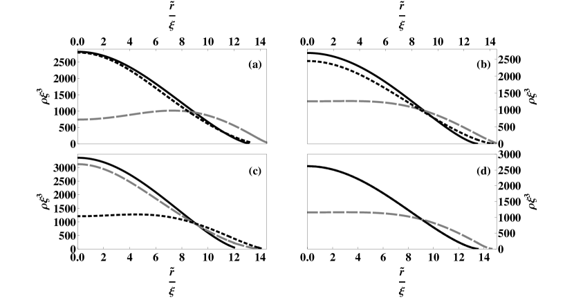
Figure 3: Density profiles of the three Fermi components for various interactions between pairs. We fixed the number of atoms in each spin state to be $N_{\sigma}\simeq 4.5\times 10^{5}$. The dimensionless scattering lengths between pairs are: (a) $\tilde{a}_{12}=1$, $\tilde{a}_{13}=-1$, and $\tilde{a}_{23}=4$, (b) $\tilde{a}_{12}=0.1$, $\tilde{a}_{13}=-1$, and $\tilde{a}_{23}=4$, (c) $\tilde{a}_{12}=-2$, $\tilde{a}_{13}=-1$, and $\tilde{b}_{23}=4$, (d) $\tilde{a}_{12}=1$, $\tilde{a}_{13}=2$, and $\tilde{a}_{23}=2$. Black line: component 1, dashed gray line: component 2, and dotted line: component 3.

For density variations, we simultaneously solve equations (11), (III), and (III) for given atom numbers in each spin states and given interactions between different pairs. In figure 3, we plot the density profiles for various interaction strengths for an atomic mixture with equal numbers in each three spin states. As seen in the figure, all three components exist in the trap center. However, the density imbalance remains finite through out the trap. The most pronouncing feature is the non-monotonic density variations of one component when both repulsive and attractive interactions are present. As a result of the spatially inhomogeneous trap, the balanced mixture of atomic cloud forms a 3-shell structure similar to the case of population imbalanced two-component gases. While the inner most shell contains all three components, the outer most shell contains only a single component. Even though, we consider a population balanced mixture in FIG. 3, we find density imbalanced throughout the trap, similar to a case of population imbalanced two-component system. It should be noted that the density imbalance in three-component system here is not due to the population imbalance but due to the different interactions between different pairs.

The density profiles of an atomic mixture with unequal populations are shown in FIG. 4. We find very similar density profiles as the case of equal population, however, depending on the number of atoms in each spin states and the interaction between different pairs, one component can completely repel from the trap center giving rise a donut shape density profile. This donut shape density profile is an unique feature of a three-component normal gas in the presence of population imbalance where as this feature is absent in a two-component gas.

For the data in FIG 3 and FIG. 4, we choose interaction parameters unsystematically to show the different behavior of density profiles. Even though the density profiles are shown as a function of scaled parameter $\tilde{r}$, the generic behavior in real space must be the same. This can be easily understood if we consider the isotropic case where $\omega_{\perp}=\omega_{z}\equiv\omega$. For this case, the atomic cloud is isotropic and the density variations can be presented as a function of $r$, just like in FIG 3 and FIG. 4.

Figure 4: Density profiles of the three Fermi components for various interactions between pairs and different numbers. The number of atoms and the dimensionless scattering lengths between pairs are: (a) $\tilde{a}_{12}=1$, $\tilde{a}_{13}=2$, and $\tilde{a}_{23}=6.6$, $N_{1}\simeq 3.0\times 10^{5}$, $N_{2}\simeq 3.0\times 10^{5}$, and $N_{3}\simeq 1.6\times 10^{5}$ (b) $\tilde{a}_{12}=-1$, $\tilde{a}_{13}=3.6$, and $\tilde{a}_{23}=2.5$, $N_{1}\simeq 6.7\times 10^{5}$, $N_{2}\simeq 6.0\times 10^{5}$, and $N_{3}\simeq 1.9\times 10^{5}$ (c) $\tilde{a}_{12}=0.462$, $\tilde{a}_{13}=1.04$, and $\tilde{a}_{23}=4.51$, $N_{1}\simeq 2.8\times 10^{5}$, $N_{2}\simeq 4.7\times 10^{5}$, and $N_{3}\simeq 6.7\times 10^{5}$ (d) $\tilde{a}_{12}=-0.1$, $\tilde{a}_{13}=-0.2$, and $\tilde{a}_{23}=-0.3$ $N_{1}\simeq 2.7\times 10^{5}$, $N_{2}\simeq 1.4\times 10^{5}$, and $N_{3}\simeq 8.8\times 10^{4}$. Black line: component 1, dashed gray line: component 2, and dotted line: component 3.

In experiments, real-space density distributions of each components can be obtained by using in situ imaging. After trapping and cooling, the system can be prepared at any desirable population. As experimental time scales are smaller than the spin relaxation time of the atoms, fixed spin population can be maintained throughout the experiment. Then by sweeping an uniform magnetic field, scattering lengths between different pairs can be set at different values. As some three-component atomic systems (for example, lowest hyperfine spin states of ⁶Li jochim ) possess three broad s-wave Feshbach resonances, by tuning scattering lengths, the interactions between different pairs can be varied. However, in a current experimental setups, interaction strengths, (i.e, the scattering lengths between different pairs) cannot be controlled independently whereas the number of atoms in each spin states can be varied independently.

Density profiles of an repulsively interacting two-component atomic gas in a harmonic trap are discussed in Ref. 2comptf1 ; 2comptf2 ; 2comptf2D ; 2compsc in the context of collective ferromagnetism. While the authors in these references discuss spontaneous magnetization and phase separations of two hyperfine spin components, Duine et al macd discuss the nature of the ferromagnetic phase transition in the mean field description and beyond mean filed theory of a homogenous system. The study in Ref. 2comptf2 is similar to the study in Refs. 2comptf1 ; 2compsc , however, authors in Ref. 2comptf2 go beyond mean field theory and study the effect of trap anisotropy on magnetization. Except Ref. 2compsc , all above studies are restricted to two-component atomic gases. Salasnich at el 2compsc investigate the density profiles of a three-component gas, however, the authors have restricted themselves to an equal and repulsive interaction between different pairs of fermions. As we have relaxed their constraints in the present study allowing to have both repulsive and attractive, as well as different interactions, we find qualitatively and quantitatively very different results.

IV IV. Dipole oscillations

By solving for the eigenvalues of Eq. 10, we find the three dipole oscillation frequencies, $\omega_{0}=\omega_{z}$ and $\omega_{\pm}=\sqrt{\omega_{z}^{2}-C\pm\sqrt{B}}$, where

$$C=\frac{1}{2}\sum_{\sigma\neq\nu}K_{\sigma\nu}(N_{\sigma}+N_{\nu})$$ (15)

and

$$B=\frac{1}{2}\sum_{\sigma\neq\nu}K_{\sigma\nu}^{2}(N_{\sigma}+N_{\nu})+$$

$$\frac{1}{2}\sum_{\sigma\neq\nu\neq\mu}K_{\sigma\nu}K_{\sigma\mu}(N_{\nu}N_{\mu}-N_{\sigma}N_{\mu}-N_{\sigma}N_{\nu}-N^{2}_{\sigma}).$$ (16)

The parameter $K_{\sigma\nu}=A_{\sigma\nu}/(mN_{\sigma}N_{\nu})$. The eigenvalue $\omega_{0}$ corresponding to the eigenvector $\eta_{1}=\eta_{2}=\eta_{3}$ and represents the in-phase oscillation frequency of the system. This mode follows the Kohn’s theorem and it is independent of interactions and the atomic population. The other two eigenvectors are $\eta_{1}/N_{1}=\eta_{2}/N_{2}=-\eta_{3}/N_{3}$ and $\eta_{1}/N_{1}=-\eta_{2}/N_{2}=\eta_{3}/N_{3}$. These two modes are corresponding to the oscillations where two components are in in-phase while the other one is in out-of-phase oscillations.

In terms of dimensionless parameters, $K_{\sigma\nu}$ is given by

$$K_{\sigma\nu}=\frac{3\pi\tilde{a}_{\sigma\nu}\omega_{z}^{2}}{N_{\sigma}N_{\nu}}\int\tilde{r}^{2}d\tilde{r}\frac{\partial\rho^{(0)}_{\sigma}}{\partial\tilde{r}}\frac{\partial\rho^{(0)}_{\nu}}{\partial\tilde{r}}.$$ (17)

In order to see the qualitative behavior of the out-of-phase oscillations, we restrict ourself to the equal population and equal interactions. For the case of equal population $N_{1}=N_{2}=N_{3}\equiv N$ and equal interactions $\tilde{a}_{12}=\tilde{a}_{13}=\tilde{a}_{23}\equiv\tilde{a}$, the out-of-phase modes are degenerate and given by

$$\biggr{(}\frac{\omega_{d}}{\omega_{z}}\biggr{)}^{2}=1-\frac{4\pi\tilde{a}}{3N}\int\tilde{r}^{2}d\tilde{r}\biggr{(}\frac{\partial\rho^{(0)}}{\partial\tilde{r}}\biggr{)}^{2}$$ (18)

where $\rho^{(0)}=\rho_{1}^{(0)}+\rho_{2}^{(0)}+\rho_{3}^{(0)}$. This density oscillation frequency as a function of interaction is shown in FIG. 5 for the case of $N=6.5\times 10^{6}$. For this case case, the size of the Fermi gas becomes larger as the interaction increases, and then the density oscillation frequency $\omega_{d}$ monotonically decreases.

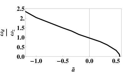
Figure 5: Out-of-phase dipole oscillation frequency as a function of interaction ($\tilde{a}$) for a symmetric system with $N=6.5\times 10^{6}$ number of atoms in each spin state. We set the interaction between different pairs of fermions to be equal.

As it has been suggested recently taylor , the out-of phase dipole mode can be excited via two-photon Bragg scattering in experiments. As the two-photon Bragg scattering spectrum is related to the dynamic structure factor, measuring the density response spectrum with available experimental techniques bragg allows one to measure the out-of phase dipole mode frequencies discussed here.

V V. Discussions and Summary

Even though, we have restricted ourselves to the zero temperature in this paper, we do not expect qualitative changes at finite temperatures. Even with the attractive interaction between some pairs, the system will be in normal state if the population imbalance is large. In the presence of attractive interactions between different pairs of fermions (and at low population imbalances), it is possible to form s-wave superfluid phases which require equal densities. Unlike a two-component Fermi gas, a three-component Fermi gas can undergo competitive BCS pairing and provide non-trivial order parameters. In the presence of a superfluid phase, superfluid region will spatially phase separate into a concentric shell surrounded by density imbalance normal shells. Even though, the experimental observations of trionic bound states and superfluid phases are yet to be observed in near future, there are series of theoretical studies on three-component superfluidity 3compsf1 ; 3compsf2 ; 3compsf3 ; 3compsf4 ; 3compsf5 .

Another promising perspective of a three-component Fermi system is to observe universal three-body quantum physics called, Efimov states. In the present work, we have neglected the appearance of an infinite number of three-body bound states (Efimov states) and two-body pairing between components. As there is no three-body interactions, three-body recombination is forbidden in a dilute two-component Fermi gas.

In summary, we use a density functional approach to investigate the Thomas Fermi density profiles and dipole oscillation frequencies of an interacting three-component normal Fermi gas at zero temperature. We constructed a phase diagram for a homogenous system at selected representative values of parameters to show that the system possesses a rich phase diagram, even neglecting the possible pairing between atom pairs. Even for an equal population atomic mixture, we find density imbalance through out the harmonic trap due to the different interaction between different pairs. For an unequal population atomic mixture, we find that one of the component completely repel from the trap center showing a donut shape atomic cloud surrounded by two concentric spherical clouds. In both cases, density profiles show dramatic deviations showing non-monotonic density distributions as opposed to the distributions seen in a two-component gas. Another qualitative difference from the two-component gas is that the density imbalance even for a population balanced normal gas. This density imbalance in the presence of population balance is due to the different interactions between different pairs. We also derive in-phase and out-of-phase dipole oscillation frequencies to show how interaction and population imbalance effect on these mode frequencies.

References

- (1) M. Grenier, C. A. Regal, and D. S. Jin, Nature 426, 537 (2003); S. Jochim, M. Bartenstein, A. Altmeyer, G. Hendl, S. Riedl, C. Chin, J. H. Denschlag, and, R. Grimm, Science 302, 2101 (2003); M. W. Zwierlein, C. A. Stan, C. H. Schunck, S. M. F. Raupach, A. J. Kerman, and, W. Ketterle, Phys. Rev. Lett. 92, 120403 (2004); G. B. Partridge, K. E. Strecker, R. I. Kamar, M. W. Jack, and R. G. Hulet, Phys. Rev. Lett. 95, 020404 (2005).
- (2) U. Fano, Phys. Rev. A 124, 1866 (1961); H Feshbach, Ann. Phys. 5, 357 (1961).
- (3) M. Bartenstein, A. Altmeyer, S. Riedl, R. Geursen, S. Jochim, C. Chin, J. H. Denschlag, R. Grimm, A. Simoni, E. Tiesinga, C. J. Williams, and P. S. Julienne, Phys. Rev. Lett. 94, 103201 (2005).
- (4) T. B. Ottenstein, T. Lompe, M. Kohnen, A. N. Wenz, and S. Jochim, Phys. Rev. Lett. 101, 203202 (2008).
- (5) J. H. Huckans, J. R. Williams, E. L. Hazlett, R. W. Stites, and K. M. O’Hara, Phys. Rev. Lett. 102, 165302 (2009).
- (6) A. N. Wenz, T. Lompe, T. B. Ottenstein, F. Serwane, G. Z rn, S. Jochim, pre-print arXiv:0906.4378.
- (7) T. Sogo and H. Yabu, Phys. Rev. A 66, 043611 (2002).
- (8) L. J. LeBlanc, J. H. Thywissen, A. A. Burkov, and A. Paramekanti, Phys. Rev. A 80, 013607 (2009).
- (9) T. Maruyama and G. F. Bertsch, Phys. Rev. A 73, 013610 (2006).
- (10) M. Ogren, K. Karkkainen, Y. Yu and S M Reimann, J. Phys. B: At. Mol. Opt. Phys. 40 2653 (2007).
- (11) R. A. Duine and A. H. Macdonald, Phys. Rev. Lett. 95, 230403 (2005).
- (12) L. Salasnich, B. Pozzi, A. Parola and L. Reatto, J. Phys. B.: At. Mol. Opt. Phys. 33, 3943 (2000).
- (13) E. Taylor, H. Hu, X. Liu, and A. Griffin, preprint arXiv: 0709.0698.
- (14) J. Stenger, S. Inouye, A. P. Chikkatur, D. M. Stamper-Kurn, D. E. Pritchard, and W. Ketterle, Phys. Rev. Lett. 82, 4569, (1999).
- (15) T. Paananen, J. -P. martikainen, and P. Torma, Phys. Rev. A 73, 053606 (2006); T. Paananen, P. Torma, and J.-P. Martikainen, Phys. Rev. A 75, 023622 (2007); T. N. De Silva, Phys. Rev. A 80, 013620 (2009).
- (16) P. F. Bedaque, Jos P. D’Incao, e-print arXiv:cond-mat/0602525; H. Zhai, Phys. Rev. A 75, 031603 (2007); G. Catelani and E. A. Yuzbashyan, Phys. Rev. A 78, 033615 (2008); L. He, M. Jin, and P. Zhuang, Phys. Rev. A 74, 033604 (2006).
- (17) R. W. Cherng, G. Refael, and E. Demler, Phys. Rev. Lett. 99, 130406 (2007); X. Liu, H. Hu, and P. D. Drummond, Phys. Rev. A 77, 013622 (2008); X. W. Guan, M. T. Batchelor, C. Lee, and H.-Q. Zhou, Phys. Rev. Lett. 100, 200401 (2008).
- (18) A. Rapp, G. Zarand, C. Honerkamp, and W. Hofstetter, Phys. Rev. Lett. 98, 160405 (2007); T. Luu and A. Schwenk, Phys. Rev. Lett. 98, 103202 (2007); A. Rapp, W. Hofstetter, and G. Zarand, Phys. Rev. B 77, 144520 (2008); S. Capponi, G. Roux, P. Lecheminant, P. Azaria, E. Boulat, and S. R. White, Phys. Rev. A 77, 013624 (2008); P. Azaria, S. Capponi, and P. Lecheminant, arXiv: 0811.0555.
- (19) G. M. Bruun, A. D. Jackson, and E. E. Kolomeitsev, Phys. Rev. A 71, 052713 (2005); N. P. Mehta, Seth T. Rittenhouse, J. P. D’Incao, and Chris H. Greene, Phys. Rev. A 78, 020701 (2008).