Radiative hydrodynamics simulations of red supergiant stars: I. interpretation of interferometric observations

Abstract

Context. It has been suggested that convection in Red Supergiant (RSG) stars gives rise to large-scale granules causing observable surface inhomogeneities. This convection is also extremely vigorous, and suspected to be one of the causes of mass-loss in RSGs. It must thus be understood in details. Evidence has been accumulated that there are asymmetries in the photospheres of RSGs, but detailed studies of granulation are still lacking. Interferometric observations offer an exciting possibility to tackle this question, but they are still often interpreted using smooth symmetrical limb-darkened intensity distributions, or very simple spotted ad hoc models.

Aims. We explore the impact of the granulation on visibility curves and closure phases using the radiative transfer code OPTIM3D. We simultaneously assess how 3D simulations of convection in RSG with CO⁵BOLD can be tested against these observations.

Methods. We use 3D radiative-hydrodynamics (RHD) simulations of convection to compute intensity maps at various wavelengths and time, from which we derive interferometric visibility amplitudes and phases. We study their behaviour with time, position angle, and wavelength, and compare them to observations of the RSG $\alpha$ Ori.

Results. We provide average limb-darkening coefficients for RSGs. We detail the prospects for the detection and characterization of granulation (contrast, size) on RSGs. We demonstrate that our RHD simulations provide an excellent fit to existing interferometric observation of $\alpha$ Ori, contrary to limb darkened disks. This confirms the existence of large convective cells on the surface of Betelgeuse.

1 Introduction

Massive stars with masses between roughly 10 and 25 M_⊙ spend some time as red supergiant (RSG) stars being the largest stars in the universe. They have effective temperatures, $T_{\rm eff}$, ranging from 3 450 to 4 100 K, luminosities of 20 000 to 300 000 L_⊙ and radii up to 1 500 R_⊙ (Levesque et al., 2005). Their luminosities place them among the brightest stars, visible to very large distances. There is however a number of open issues. They shed large amounts of mass back to the interstellar medium, but their mass-loss mechanism is unidentified, although Alfvén and acoustic waves have been proposed (Hartmann & Avrett, 1984; Pijpers & Hearn, 1989; Cuntz, 1997), as well as acoustic waves and radiation pressure on molecules (Josselin & Plez, 2007). Their chemical composition is largely unknown, despite the work of e.g. Carr et al. (2000), and Cunha et al. (2007), due to difficulties in analysing their spectra with broad, asymmetric lines with variations suspected to stem from a convection pattern consisting of large granules and (super-)sonic velocities (Josselin & Plez, 2007; Gray, 2008). Progress has been made recently, with their $T_{\rm eff}$-scale being revised both at solar and Magellanic Clouds metallicities using 1D hydrostatic models (Levesque et al., 2005, 2006; Massey et al., 2007; Levesque et al., 2007). Although these MARCS models (Gustafsson et al., 2008) give a good fit of the optical spectra allowing the derivation of $T_{\rm eff}$ and reddening, problems remain. There is a blue-UV excess in many of the observed spectra, that may point to scattering by circumstellar dust, or to an insufficiency in the models. There is also a mismatch in the IR colours, that could be due to atmospheric temperature inhomogeneities characteristic of convection (Levesque et al., 2006).

In recent years, hydrodynamical modeling of convection in RSGs has lagged behind that of solar type stars due to the necessity to include the whole star in the simulation box. Freytag et al. (2002) have succeeded in doing such numerical simulations of a typical RSG. We have thus engaged in an important effort to improve our understanding and description of RSGs using detailed numerical simulations and a large set of observational material.

This paper is the first in this series and it is aimed to explore the granulation pattern of RSGs and its impact on interferometric observations.

2 3D radiative transfer in Radiative-hydrodynamics simulation

2.1 3D hydrodynamical simulations with CO⁵BOLD

The numerical simulations employed in this work have been obtained using CO⁵BOLD (Freytag et al., 2002; Freytag & Höfner, 2008) in the star-in-a-box configuration: the computational domain is a cube, and the grid is equidistant in all directions. All six faces of the cube use the same open boundary conditions for material flows and emergent radiation. In addition, there is an ”inner boundary condition”: in a small spherical region in the center of the cube a source term to the internal energy provides the stellar luminosity and a drag force brakes dipolar flows through it. Otherwise, the hydrodynamics and the radiative transfer scheme do not notice the core and integrate right through it. Radiation transport is strictly in LTE. The grey Rosseland mean opacity is a function of gas pressure and temperature. The necessary values are found by interpolation in a table which has been merged at around 12 000 K from high-temperature OPAL data (Iglesias et al., 1992) and low-temperature PHOENIX data (Hauschildt et al., 1997) by Hans-Günter Ludwig. Some more technical information can be found in Freytag & Höfner (2008), the CO⁵BOLD Online User Manual (www.astro.uu.se/~bf/co5bold$\_$main.html), and in a forthcoming paper by Freytag (2009).

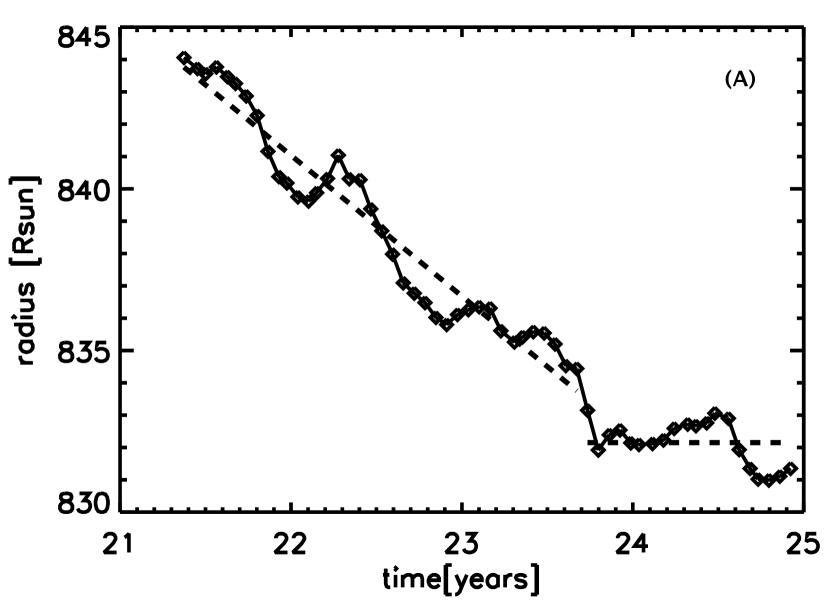
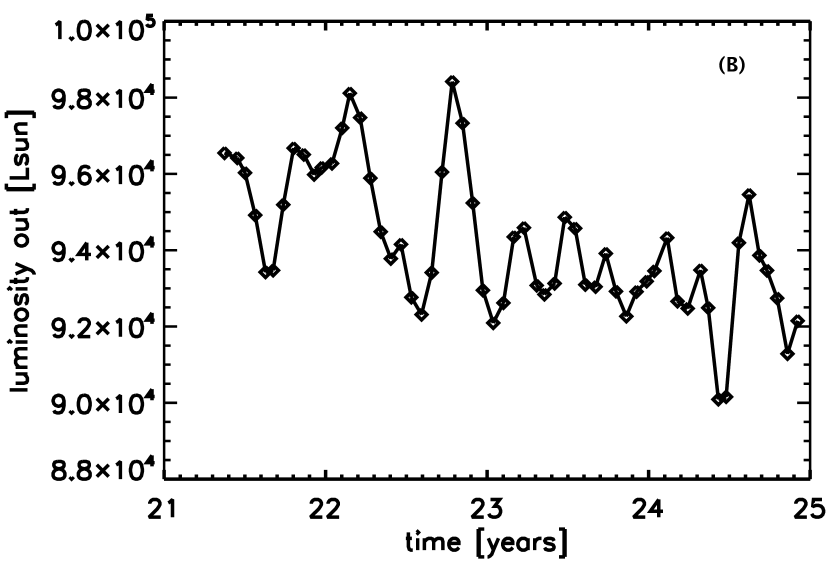
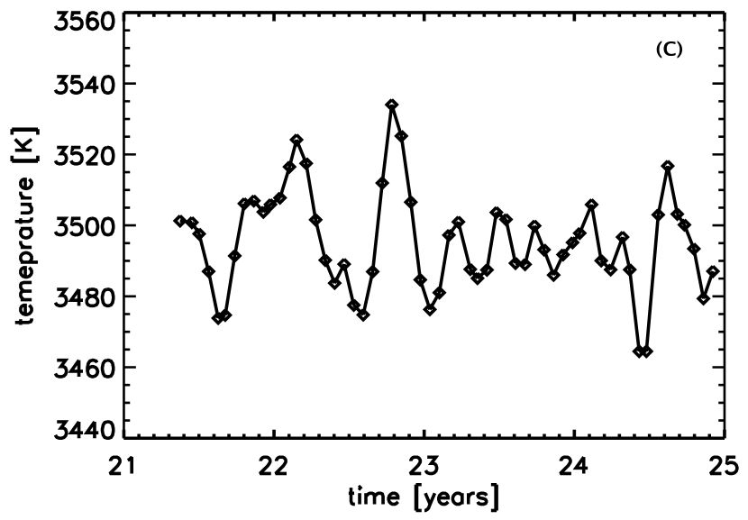
The 12 M_⊙ model we use in this paper (st35gm03n07) is the result of intensive calculations which have led to about 7.5 years of simulated stellar time. It has a numerical resolution of 8.6 R_⊙ in a cube of 235³ grid points. The model parameters are a luminosity of $L=93000\pm 1300\leavevmode\nobreak\ {\rm L}_{\odot}$, an effective temperature of $T_{\rm{eff}}=3490\pm 13\leavevmode\nobreak\ K$, a radius of $R=832\pm 0.7\leavevmode\nobreak\ {\rm R}_{\odot}$, and followingly a surface gravity ${\rm log}\leavevmode\nobreak\ g=-0.337\pm 0.001$. These values are averages over spherical shells and over time (over the last year), and the errors are one sigma fluctuations with respect to the average over time. We define the stellar radius, $R$, and the effective temperature, $T_{\rm{eff}}$, as follows. First, we compute the average temperature and luminosity over spherical shells, $T(r)$, and $L(r)$. We then search the radius $R$ for which ${L(R)}/(4\pi R^{2})=\sigma T^{4}(R)$, where $\sigma$ is the Stefan-Boltzmann constant. The effective temperature is then $T_{\rm{eff}}=T(R)$. Fig. 1 shows the value of the radius, temperature and luminosity over the last 3.5 years. The radius drifts by about $-0.5\%$ per year and seems to have stabilised to $R=832\leavevmode\nobreak\ {\rm R}_{\odot}$ in the last year. $T_{\rm eff}$ fluctuates by $\pm 1\%$ over the whole sequence, with a constant average. The luminosity fluctuations are of the order of $\pm 4\%$, reflecting the temperature variations, with a decrease of about $1\%$ per year in the first years, reflecting the radius decrease. These drifts indicate that the simulation has not completely converged in the first years. In this work we consider the whole 3.5 year sequence, despite the small radius drift, in order to have better statistics. The preceding 4 years of the simulation are not considered here, since they show larger drifts. The interferometric observables derived in this work are not sensitive to the drift of the parameters.

This is our ”best” RHD simulation so far because it has stellar parameters closest to real RSGs (e.g., 3650 K for $\alpha$ Ori, Levesque et al., 2005). New simulations with different stellar parameters are in progress and they will be analyzed in a forthcoming paper.

Figure 1: Radius (Panel A), luminosity (Panel B) and temperature (Panel C) as a function of time for the simulation used in this work. The radius is fitted with the law: $R(t)=936.9-4.3\times t$ for $t\leq 23.8$ yrs years and $R=832$ R_⊙ for $t>23.8$ yrs.

2.2 Radiative transfer code: OPTIM3D

We have developed a 3D pure LTE radiative transfer code, OPTIM3D to generate synthetic spectra and intensity maps from snapshots of the 3D hydrodynamical simulations, taking into account the Doppler shifts caused by the convective motions. The radiation transfer is calculated in detail using pre-tabulated extinction coefficients generated with the MARCS code (Gustafsson et al., 2008). These tables are functions of temperature, density and wavelength, and were computed with the solar composition of Asplund et al. (2006). The tables include the same extensive atomic and molecular data as the MARCS models. They were constructed with no micro-turbulence broadening and the temperature and density distribution is optimized to cover the values encountered in the outer layers of the RHD simulations. The wavelength resolution is $R=\lambda/\Delta\lambda=500\,000$ and we checked that this resolution is sufficient to ensure an accurate calculation of broadened line profiles of RSGs even after interpolation of the opacity at the Doppler shifted wavelengths.

The monochromatic intensity emerging towards the observer at a given position on the simulation can be computed by integrating the source function along a ray perpendicular to a face of the cube, at that position. In LTE it reads:

$${I}_{\lambda}\left(0\right)=\int^{\tau_{\lambda}}_{0}S_{\lambda}\left({t_{\lambda}}\right)e^{-{t_{\lambda}}}d{t_{\lambda}}$$ (1)

where $I_{\lambda}$ is the intensity, $t_{\lambda}$ is the optical depth along the ray increasing inwards, $\tau_{\lambda}$ is the maximum optical depth reached along the line-of-sight, and $S_{\lambda}=B_{\lambda}\left(T\right)$, the Planck function at the temperature $T$, is the source function. A Gauss-Laguerre quadrature of order $n$ can be performed to evaluate the integral, Eq. (1), when $\tau_{\lambda}\rightarrow\infty$. This method is much faster than a detailed integration along the discretized ray, as it uses only the value of the source function at $n$ depth points weighted with $n$ predetermined weights. This method is reliable as long as the source function is sufficiently smooth along the optical depth scale, and is well known at the quadrature points. This is not always the case in our simulations where the optical depth scale may jump by large amounts between 2 successive cells, e.g. from $\tau=1$ to $\tau=300$ for extreme cases. The source function must then be interpolated at intermediate optical depths, and the result is largely dependent on the way this interpolation is performed. Note however that this is also the case for a detailed integration, where too large jumps in the source function or optical depth scale will cause uncertainties in the resulting intensity. We checked for differences between a Gauss-Laguerre quadrature and a detailed summation of the contributions from all cells, with different kinds of interpolations, and found differences in intensities emerging from a single ray of less than $10\%$ on average, with some extreme cases reaching more than $100\%$ due to a particularly illconditioning of the source function. The average differences being in an acceptable range, we therefore rely on the Gauss-Laguerre quadrature, with a linear interpolation of the source function on the logarithmic $\tau$-scale. The quadrature points and weights we use are listed in Tab. 1 (Abramowitz & Stegun, 1972). For the rays where the optical depth does not reach high enough values, we carry a detailed summation of the contribution from all cells along the ray.

In practice, once the input simulation is read, OPTIM3D interpolates the opacity tables in temperature and logarithmic density for all the simulation grid points using a bi-linear interpolation. The interpolation coefficients are computed only once, and stored. Bi-linear interpolation has been preferred to spline interpolation because: (i) spline is significantly more time consuming, (ii) and comparisons with other codes do not show great improvements using splines (see below). Then, the logarithmic extinction coefficient is linearly interpolated at each Doppler-shifted wavelength in each cell along the ray, and the optical depth scale along the ray is calculated. Eq. (1) is then integrated, giving the intensity emerging towards the observer at that wavelength and position. This calculation is performed for every line-of-sight perpendicular to the face of the computational box, and for all the required wavelengths.

Table 1: Gauss-Laguerre quadrature weights for n=10.

$$\begin{array}[]{p{0.5\linewidth}l}\hline\cr\hline\cr\vskip 3.0pt plus 1.0pt minus 1.0pt\cr{\rm abscissa}&{\rm weight}\\ \vskip 3.0pt plus 1.0pt minus 1.0pt\cr\hline\cr\vskip 3.0pt plus 1.0pt minus 1.0pt\cr 0.137793470540&3.08441115765E-01\\ 0.729454549503&4.01119929155E-01\\ 1.808342901740&2.18068287612E-01\\ 3.401433697855&6.20874560987E-02\\ 5.552496140064&9.50151697518E-03\\ 8.330152746764&7.53008388588E-04\\ 11.843785837900&2.82592334960E-05\\ 16.279257831378&4.24931398496E-07\\ 21.996585811981&1.83956482398E-09\\ 29.920697012274&9.91182721961E-13\\ \vskip 3.0pt plus 1.0pt minus 1.0pt\cr\hline\cr\end{array}$$

Comparisons with existing codes were carried out. The spectral synthesis code Turbospectrum (Plez et al., 1993, Alvarez & Plez, 1998, and further improvements by Plez) was used with one-dimensional MARCS models, where the source fonction is very well sampled on the $\tau$-scale. OPTIM3D computations made with bi-linear interpolation deviate by less than $5\%$, and the deviation decreases to 0.2$\%$ with spline interpolation. We also checked OPTIM3D against Linfor3D (Cayrel et al., 2007 for the Non-LTE version, and http://www.aip.de/~mst/Linfor3D/linfor_3D_manual.pdf for the LTE version) using 3D CO⁵BOLD local models. We compared synthetic spectra computed for three artificial iron lines (with increasing strength) centered at a laboratory wavelength of 5500 Å and using the same abundances. The discrepancy between the results of the codes is less than 3$\%$ and it becomes even less than 0.2$\%$ when a spline interpolation of the opacity tables is used in OPTIM3D (with a significant increase of the CPU time). Finally, comparisons were made with the spectral line formation code used by, e.g., Asplund (2000) for 3D local convection simulations carried out with the code by Stein & Nordlund (1998) for giant stars (Collet et al., 2007). The tests have been carried out on the [OI] line at 6300.3 Å and various Fe I and Fe II lines around 5000 Å. The discrepancies between the resulting synthetic spectra are less than 2$\%$, and become even less than 0.6$\%$ when a spline interpolation of the opacity tables is used in OPTIM3D. Thus, the interpolation is the main source of error. In conclusion, if only a few lines are computed for, e.g., accurate abundance determinations, Linfor3D or the Asplund code are better because they mostly avoid interpolations into opacity tables. The code used by Asplund performs bi-cubic interpolations of the continuum opacity and of the individual number densities, whereas we interpolate the total opacity from all lines contributing at a given wavelength, which is in principle less accurate. So, when a large wavelength range must be calculated taking into account many molecular and atomic lines simultaneously, OPTIM3D is a better, faster choice, that still provides a result accurate to a few percents.

3 Simulated images in the H and K bands: giant convective cells

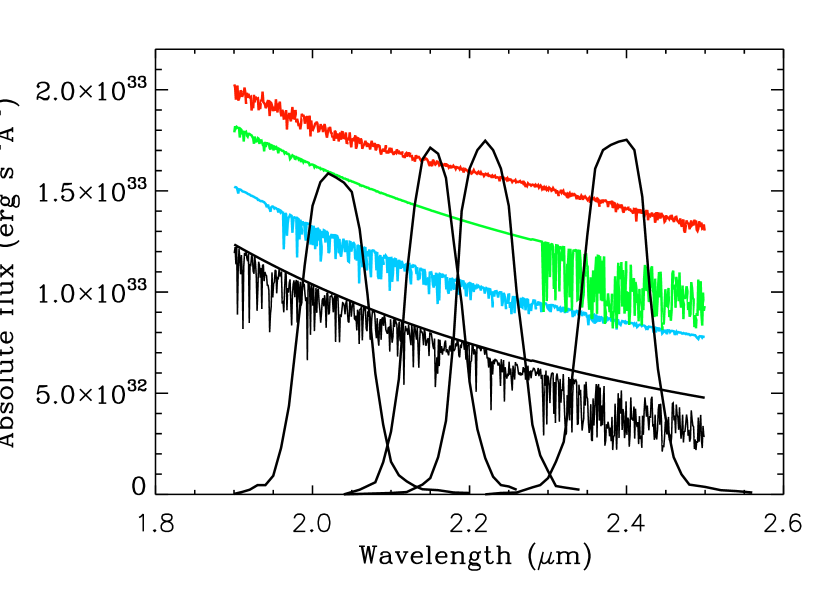
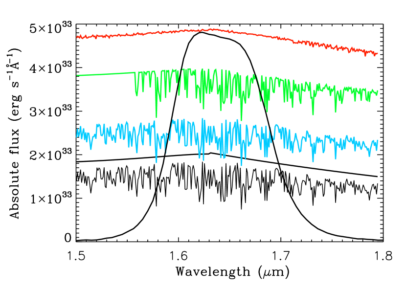
In this work, we analyze the properties of the simulations in the H and K bands where many interferometric observations have been done, and existing interferometers, e.g. VLTI/AMBER, operate routinely. We calculated intensity maps for a series of snapshots about $23$ days apart covering 3.5 years of the model described above. We use the transmission curve of the four K band filters mounted on FLUOR (Fiber Linked Unit for Optical Recombination; Coude Du Foresto et al., 1998), and of the H band filter mounted on IONIC (Integrated Optics Near-infrared Interferometric Camera; Berger et al., 2003) at the IOTA interferometer (Traub et al., 2003). The K band filters (Fig. 2) are: K203 (with a central wavelength of $2.03$ $\mu$m), K215 ($2.15$ $\mu$m), K222 ($2.2$ $\mu$m), and K239 ($2.39$ $\mu$m).

Figure 2: The transmission curves of the 4 narrow band filters mounted on the FLUOR instrument at IOTA together with the K band synthetic spectrum of a snapshot of the simulation and the corresponding continuum (bottom black curve). From the top, the spectra computed with only H₂O (red), only CO (green), and only CN (blue) are shown with an offset of respectively $0.9\times 10^{33}$, $0.6\times 10^{33}$ and $0.3\times 10^{33}$ erg cm^-2 s^-1 Å^-1.

The H band filter has a central wavelength of $1.64$ $\mu$m (Fig. 3). The resulting intensities reported in this work are normalized to the filter transmission as: $\frac{\int I_{\lambda}T\left(\lambda\right)d\lambda}{\int T\left(\lambda\right)d\lambda}$ where $I_{\lambda}$ is the intensity and $T\left(\lambda\right)$ is the transmission curve of the filter at a certain wavelength. The intensity maps are showed after applying a median [3x3] smoothing (see Section 5).

Figure 3: The transmission curve of the filter mounted on IONIC at IOTA together with the H band synthetic spectra computed as in Fig. 2. From the top, the offset of the spectra is $3\times 10^{33}$, $2\times 10^{33}$, and $1\times 10^{33}$ erg cm^-2 s^-1 Å^-1.

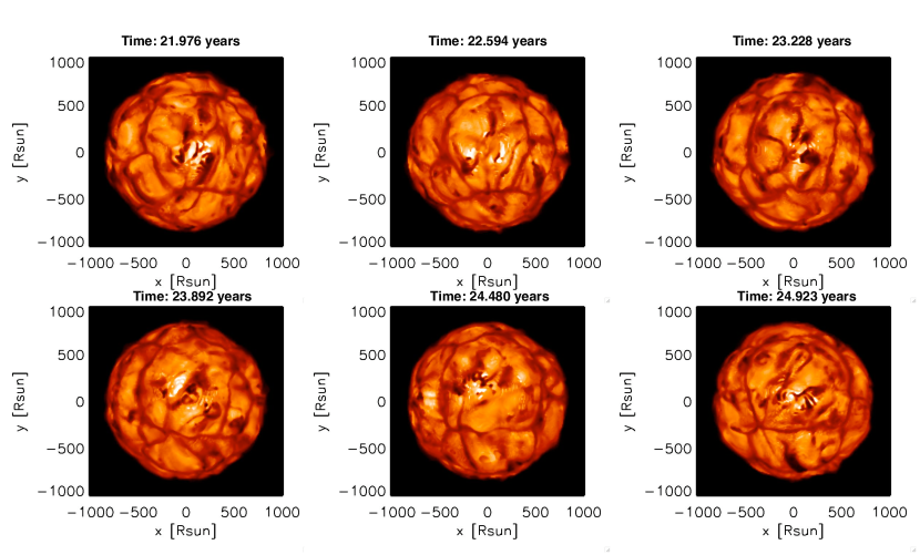
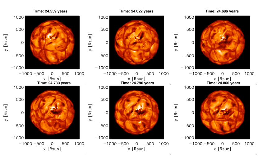
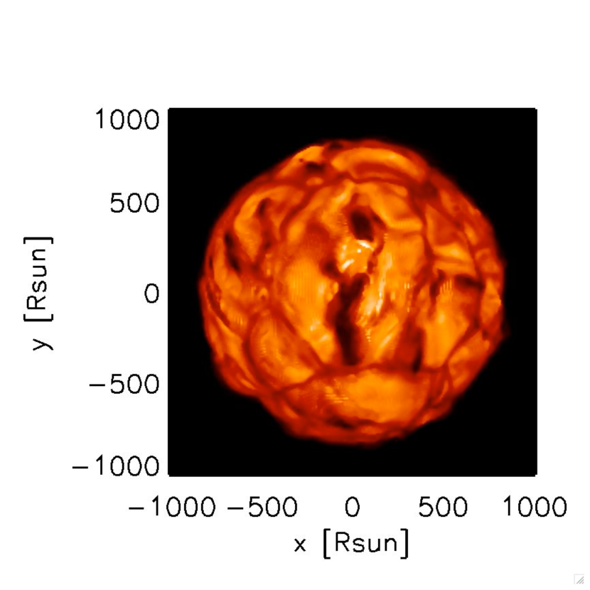
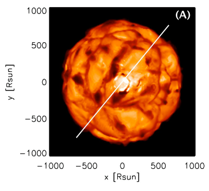
It can be seen from our simulations (see Fig. 4) that the surface of the stellar model is covered by few large convective cells of a size of about 400 to 500 R_⊙ that evolve on a time-scale of years. These cells have strong downdrafts that can penetrate down to the stellar core (Freytag et al. 2002, and 2009, in preparation). Near the surface, there are short-lived (a few months to one year) small-scale (50 to 100 R_⊙) granules (bottom panels of Fig. 4). Freytag et al. (1997) found a relation between the mean horizontal size of convective granules $x_{\rm{gran}}$ and the atmospheric pressure scale-height defined as $H_{p0}=\frac{kT_{\rm{eff}}}{g\mu m_{\rm{H}}}$ for GK dwarfs and subgiants. It is unclear if such a relation can be extrapolated to 3D simulations of RSGs. Using it we find $x_{\rm{gran}}/R_{\star}=10\times H_{p0}/R_{\star}=0.1$, for parameters appropriate for a RSG atmosphere dominated by gas pressure. Obviously, this leads to a size much smaller than what can be seen in Fig. 4. Freytag et al. (1997) found that a value of $x_{\rm{gran}}/H_{p0}=10$ would fit 2D simulations for GK dwarfs and subgiants, but they show also that A-type and F-type stars lie above the curve indicating that they have larger granules. These stars have large turbulent pressure that may dominate over the gas pressure in turbulent convective layers. Following Gustafsson et al. (2008), we write $P_{\rm{turb}}=\beta\rho v_{\rm{turb}}^{2}$, where $v_{\rm{turb}}$ is the turbulent velocity, $\rho$ is the gas density, and $\beta$ is a parameter close to one, whose value depends on the anisotropy of the velocity field. A better way to express $H_{p0}$ is thus $H_{p0}=\frac{kT_{\rm{eff}}}{g\mu m_{\rm{H}}}\left(1+\beta\gamma\left(\frac{v_{\rm{turb}}}{c_{s}}\right)^{2}\right)$, where $\gamma$ is the adiabatic exponent, and $c_{s}$ the sound speed. If $v_{\rm{turb}}$ is only a factor 2 larger than $c_{s}$, $H_{p0}$ is increased by a factor of about 5. This is the case for our RSG simulation where $P_{\rm{turb}}/P_{\rm{gas}}\sim 2$ at the surface, $R_{*}$, as determined in Sect. 2.1. This gives then $x_{\rm{gran}}/R_{\star}$=0.5, extrapolating Freytag et al. (1997) formula. This is more consistent with the large granules visible on intensity maps in Fig. 4. There are further mechanisms that might influence the size of the granules: (i) in RSGs, most of the downdrafts will not grow fast enough to reach any significant depth before they are swept into the existing deep and strong downdrafts enhancing the strength of neighboring downdrafts; (ii) radiative effects and smoothing of small fluctuations can cause an enhancement of growth time for small downdrafts while the granule crossing time is short due to large horizontal velocities; (iii) sphericity effects, see for example Freytag & Ludwig (2007), and Steffen & Freytag (2007); (iv) Freytag et al. (1997) use the effective temperature and the pressure scale height at the bottom of the photosphere as reference, however, also layers below the photosphere can matter; (v) numerical resolution (or lack of it) could matter.

Figure 4: Top 6 panels: maps of the intensity in the IONIC filter (linear scale with a range of [0;$2.5\times 10^{5}$] erg cm^-2 s^-1 Å^-1). The different panels correspond to snapshots separated by 230 days ($\sim 3.5$ years covered). Bottom 6 panels: successive snapshots separated by 23 days ($\sim 140$ days covered).

4 Intensity profiles

The simulated RSG atmospheres appear very irregular, permeated with structure and dynamics. The surface inhomogeneities and their temporal evolution induce strong variations of the emerging spectra, and intensity profiles. In this section we analyse the average centre-to-limb intensity profiles, and their time variations.

4.1 Surface inhomogeneities and temporal evolution

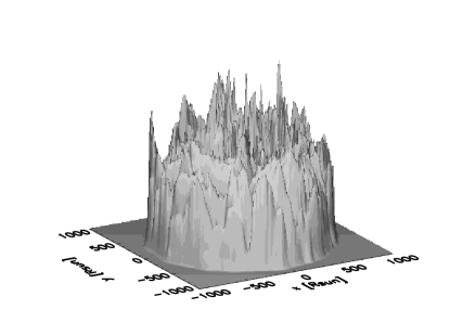
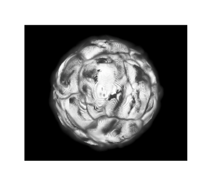
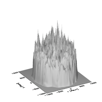
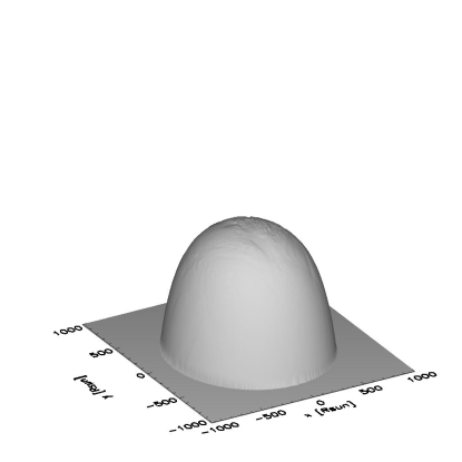
The top left panel of Fig. 5 shows a three-dimensional image representation of the intensity emerging from one face of a snapshot of the simulation in the H band. The K band appearance is similar. This image shows very sharp intensity peaks two to three pixels wide. This is also noticeable in the top right panel of the Figure as small bright (up to $40\%$ brighter than the surrounding points) patches. These patches result from the ill-conditioning of the source function, due to the lack of spatial resolution around $\tau_{\lambda}=1$ along some lines of sight where the source function may have a large jump (see Sect. 2.2). Attempts have been made to solve this problem through the interpolation of the source function and opacity inside CO⁵BOLD, but they caused numerical instabilities. The unique solution is to increase the number of grid points, and that necessitates larger and faster computers.

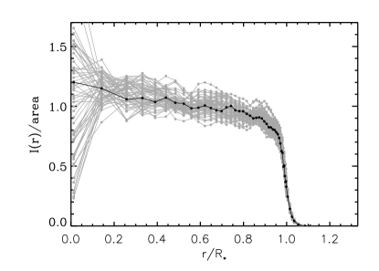
Radial intensity profiles within a given snapshot show large variations with position angle of their radial extension of about $10\%$ (see bottom left panel of Fig. 5). The variation with time of the intensity profiles are of the same order of magnitude (10$\%$, see bottom right panel of Figure).

Figure 5: Top left panel: three-dimensional image of a snapshot from Fig. 4. Top right panel: Intensity map of the same snapshot represented using the histogram equalization algorithm in order to underline the thin bright patches due to the undersampling of the $\tau$ scale. Bottom left panel: intensity profiles for three position angles of the same snapshot. The numerical box edge is at impact parameter $r/R_{\star}\sim 1.3$. The intensity is normalized to the intensity at disk center. Bottom right panel: radially averaged intensity profiles for all the snapshots of the simulation (grey); one snapshot of the simulation is emphasized with a solid black line. The intensity is normalized to the area subtended by the curve, area$=\int_{0}^{1.3}I\left(r/R_{\star}\right)dr/R_{\star}$.

4.2 The limb darkening law

Despite the large azimuthal variations of the intensity profiles, and their temporal variations, it is interesting to derive radially averaged intensity profiles for each snapshot. These may be be used, e.g., as a first approximation to interpret interferometric observations, in replacement of limb-darkening (LD) laws computed from hydrostatic models (Claret, 2000). Bottom right panel of Fig. 5 shows all the radially averaged intensity profiles obtained from the simulation.

We use a LD law of the form :

$$\frac{I(\mu)}{I(1)}=\sum_{k=0}^{3}a_{k}\left(1-\mu\right)^{k}$$ (2)

where $I(\mu)$ is the intensity, $a_{k}$ are the LD coefficients and $\mu=cos\theta$ with $\theta$ the angle between the line of sight and the radial direction. $\mu$ is related to the impact parameter $r/R_{\star}$ through $r/R_{\star}=\sqrt{1-\mu^{2}}$, where R_⋆ is the stellar radius determined as in Sect. 2.1. The average intensity profiles were constructed using rings regularly spaced in $\mu$ for $\mu\leq 1$ (i.e., $r/R_{\star}\leq 1$), and adding a few points for $r>R_{\star}$ up to the numerical box limit. The standard deviation of the average intensity, $\sigma_{I\left(\mu\right)}$, was computed within each ring. There is a small tail at $r>R_{\star}$ that gives a minor contribution to the total flux (less than 1$\%$, see bottom right panel of Fig. 5), and cannot be fitted with Eq. 2. We fitted the radially average profiles of all the snapshots of the simulation (57 profiles 23 days apart covering 3.5 years). The fit was weighted by $1/\sigma_{I\left(\mu\right)}$ in order to decrease the importance of central points with poor statistics. The fit was first made on $I(\mu)/I_{\rm{norm}}$, with $I_{\rm{norm}}$ the intensity normalized to the area subtended by the curve: $I_{\rm{norm}}=\frac{I\left(r/R_{\star}\right)}{\int_{0}^{1.3}I\left(r/R_{\star}\right)dr/R_{\star}}$. This was done in order to diminish the impact of intensity fluctuations between snapshots on the fitting coefficients.

In Tab. 2, we give the values of the four LD coefficients averaged over all 3.5 years, and renormalized to disk center, for the IONIC H-band filter, and for the K222 filter (because the sensitivity of the FLUOR instrument is always better in the continuum than in molecular bands Perrin et al., 2004b, and it samples the maximum transmission region of the K band). Fig. 6 shows an example of LD fit. The intensity profiles for different position angles for the same snapshot being very different (see Fig. 5, bottom left panel), the fitting coefficients are very scattered. The time averaged LD fits give however an indication of the shape of the intensity profile in the H and K bands (note that they are very similar). They are of course very different from simple first order LD laws. They also differ from LD laws calculated by Claret (2000) for parameters appropriate for RSGs (see Fig. 7). When comparing to observations of RSGs, we recommend to use our fits. Ideally one should use single snapshots as we do below in our analysis of Betelgeuse, as they may deviate from the average LD fit by large amounts (see Tab. 2).

Figure 6: Example of a LD fit (dashed line) using the LD law described in the text for the radially averaged intensity profile (solid line) emphasized in Fig. 5 (bottom right panel). The intensity is normalized to the area subtended by the curve. This best fit has a $\chi^{2}=0.02$.

Figure 7: The time averaged H-band radial intensity profile of our simulation (solid line), and the fit of Tab. 2 (dashed line). A fully LD (dash-dotted line), a partially LD (triple dot-dashed line), and a LD fit from Claret (2000, dotted line) for comparable RSG parameters are plotted for comparison.

Table 2: Time-averaged limb-darkening coefficients for the RHD simulation (see Eq. 2. $\sigma$ is the standard deviation over time (57 profiles covering 3.5 years.

$\lambda$	$a_{0}$	$\sigma$	$a_{1}$	$\sigma$	$a_{2}$	$\sigma$	$a_{3}$	$\sigma$
($\mu$m)		($\%$)		($\%$)		($\%$)		($\%$)
1.64	1.00	5	-0.93	50	2.03	50	-1.98	55
2.22	1.00	5	-0.85	50	2.12	45	-2.13	45

5 Visibility curves and phases

5.1 Computation

The granulation pattern has a significant impact on interferometric visibility curves and phases. We try here to derive their characteristic signature.

We compute visibilities and phases using the IDL data visualization and analysis platform. For each image, a discrete Fourier transform is calculated. In order to reduce the problems due to the finite size of the object and to avoid edge effects, the resolution in the Fourier plane is increased by padding the input $235\times 235$ pixels image with zeros up to a size of $2048\times 2048$ pixels. The visibility $V$ is defined as the modulus $|z|$, of the complex Fourier transform, $z=x+iy$, normalized to the modulus at the origin of the frequency plane, $|z_{0}|$, with the phase $\tan\theta=\Im(z)/\Re(z)$. When dealing with observations, the natural spatial frequency unit is arcsec^-1. As we study theoretical models, we use instead R${}_{\odot}^{-1}$ units. The conversion factor between these is

$$V\leavevmode\nobreak\ [arcsec^{-1}]=V\leavevmode\nobreak\ [{\rm R}_{\odot}^{-1}]\cdot d\leavevmode\nobreak\ [{\rm pc}]\cdot 214.9,$$ (3)

where 214.9 is the astronomical unit expressed in solar radii, and $d$ is the distance of the observed star. The relation between the baseline, $B$ (in m), of an interferometer, and the spatial frequency $\nu$ (in arcsec^-1) observed at a wavelength $\lambda$ (in $\mu{\rm m}$) is $\nu=B/\lambda/0.206265$. As our calculated images are affected by the source function jumps, we investigated how the visibility curves are affected by the resulting bright spikes (Fig. 5). We compare in Fig. 8 the visibility curves computed for one projected baseline from the raw image, and after applying a median $[3\times 3]$ smoothing effectively erasing the artifacts. The visibility curves are affected by these artifacts mostly for frequencies greater than 0.03 R${}^{-1}_{\odot}$ (corresponding to 33 R_⊙, i.e., $\sim$4 pixels). We can therefore apply this cosmetic median filter, as it will not affect the visibilities at lower frequencies, that are the only ones to be observable in practice with modern interferometers.

Figure 8: The solid line is the visibility curve for the IONIC filter intensity map of Fig. 5 (top right). The dotted line is computed for the same map after applying a $[3\times 3]$ median smoothing.

We now study the first few lobes of the visibility curves of our simulations, and how they are affected by asymmetries and surface structure.

5.2 The first lobe

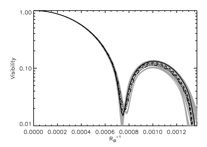
The first lobe of the visibility curve is mostly sensitive to the radial extension of the observed source. Fig. 9 (bottom panel) shows the visibility curves computed for 36 different angles from the intensity map of one snapshot in the IONIC filter (top panel). A dispersion of the visibility curves (thin grey lines in Fig. 9) is noticeable. This behavior is similar for all the snapshots. These synthetic visibilities have been compared to a uniform disk (UD) model (solid line in Fig. 9), and with limb-darkened (LD) models. We use both a fully limb-darkened disk ($I_{\mu}/I_{1}=\mu$, dotted-dashed line in the Figure), and a partially limb-darkened model with $a_{1}=-0.5$ ($I_{\mu}/I_{1}=0.5+0.5\cdot\mu$, dashed line in the Figure). The radius determined by fitting a UD disk model to the computed visibilities ranges from 794 to 845 R_⊙ for the 36 angles, up to 5$\%$ smaller than $R_{\star}$=836.5 R_⊙, the radius of the simulation determined as described in Sect. 2.1. The partially-, and fully-darkened models are respectively $\sim 2\%$, and only $\sim 1\%$ smaller than $R_{\star}$. In Fig. 9 is also shown the visibility amplitude resulting from our average LD fit of Tab. 2. The resulting diameter is then 842 R_⊙, very close to the simulation radius. Note, that Nardetto et al. (2006) also found that the UD radius is about 4 to 5$\%$ smaller than the photospheric radius of their simulation of Cepheids, and that the LD radius is much closer to the radius of their simulation. Stellar diameters determined with UD or LD fits of observed first visibility lobe of RSGs will be affected by these systematic errors. As will be shown below, observations of higher spatial frequencies will greatly improve the knowledge of the limb-darkening, and of asymetries, thus helping in better constraining the radius as well.

It is interesting to compare the angular and temporal visibility fluctuations at one sigma, defined as $F=\sigma/\rm{vis}$: (i) the temporal evolution, fixing one angle and following the RHD simulation for 3.5 years with a time-step of $\sim$23 days; (ii) the angular evolution, considering a single snapshot and computing the visibilities for 36 different angles 5^∘ apart. Fig. 10 shows that, in the first lobe, temporal and angular fluctuations have the same order of magnitude. The fluctuations are less than 1$\%$ at frequency $\sim$0.00040 R${}^{-1}_{\odot}$ (at this frequency, the visibility is greater than $50\%$), they are $\sim 3\%$ at frequency 0.00057 R${}^{-1}_{\odot}$, and are close to $\sim 10\%$ at 0.00069 R${}^{-1}_{\odot}$.

Figure 9: Top panel: intensity map in the IONIC filter (the range is [0;$2.5\times 10^{5}$] erg cm^-2 s^-1 Å^-1). Bottom panel: visibility curves from the above snapshot computed for 36 different angles 5^∘ apart (thin grey lines). Note the logarithm visibility scale. The solid black curve is a UD model, with a radius of 810 R_⊙. The dashed black line is a partially LD disk with a radius of 822 R_⊙. The dot-dashed line is a fully LD disk with a radius of 830 R_⊙. the triple-dot-dashed line is our average LD law (cf. Tab. 2) for a radius of 842 R_⊙. The stellar parameters of this snapshot are: $L=98\,400\,{\rm L}_{\odot}$, $R_{*}=836.5\,{\rm R}_{\odot}$, $T_{\rm eff}=3534$ K and $\log\leavevmode\nobreak\ g=-0.34$.

Figure 10: standard deviation of the visibility normalized to the visibility in the first lobe. The solid line indicates the temporal fluctuations for one fixed angle over 3.5 years. The trend is similar for the other angles. The dashed curve corresponds to the angular fluctuations of the snapshot in Fig. 9.

5.3 The second, third and fourth lobes: signature of the convection

As in Sect. 5.2, we analyze the angular, and temporal visibility fluctuations at one sigma with respect to the average value in the H band (IONIC filter). Fig. 11 shows an enlargement of the the second, third and fourth lobes of the visibility curves computed for different position angles. The dispersion increases clearly with spatial frequency, and visibilities deviate greatly from the UD or LD cases, due to the small scale structure on the model stellar disk.

Figure 11: Same as Fig. 9 for the second, third, and fourth lobes. In addition, the dotted line is the visibility curve for the particular azimuth parallel to the x-axis of the IONIC intensity map of Fig. 9.

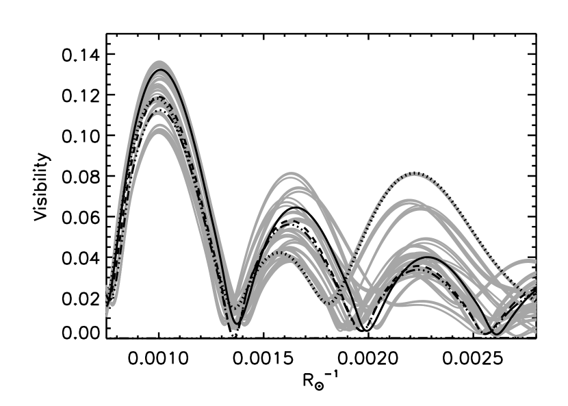
The same is true for temporal fluctuations of the visibility at a given position angle. Fig. 12 shows the temporal fluctuations of the visibilities for one fixed position angle, as well as the angular fluctuations for the snapshot of Fig. 9. As for the first lobe, there is no clear distinction between angular and temporal fluctuations. Relative fluctuations are of course large around the minima of visibility, where visibilities are also more difficult to measure. However, with the precision of current interferometers (e.g., 1$\%$ for visibilities of $\sim 5-10\%$ for VLTI-AMBER), it should be possible to characterize the granulation pattern on RSGs. This requires observing the third and the fourth lobes and not limiting the observation at the first and second lobes, that give only an information on the radius and LD. The signal to be expected in these lobes is higher than the UD or LD predictions (see dashed line in Fig. 11). Efforts should therefore be put on observing at these frequencies.

Figure 12: Same as Fig. 10 for the second, third, and fourth lobe.

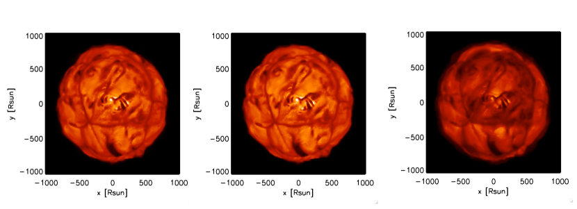
It may however turn out that approximations in our modelling (e.g., limited spatial resolution, grey radiative transfer) significantly affect the intensity contrast of the granulation. Indeed, the radiation transfer in our RHD models uses a frequency-independent grey treatment to speed up the calculations. This approximation leads to errors in the mean temperature structure in the optically thin layers that are difficult to quantify. The implementation of non-grey opacities can decrease the temperature fluctuations compared to the grey case (e.g., Ludwig et al., 1994, for local RHD models). As a consequence, the intensity contrast will be decreased, reducing the visibility fluctuations. To investigate its impact on visibilities, we artificially decrease the intensity contrast on one of our images. we use the snapshot with its nominal intensities as reference. We first fit a LD law (as in Sect 4) to the radially average intensity profile. After subtracting this average profile from the intensity map we are left with the fluctuations caused by granulation. We measure the contrast $C_{\rm{ref}}$=$\frac{I_{\rm{max}}-I_{\rm{min}}}{I_{\rm{max}}+I_{\rm{min}}}$. It is then easy to scale that contrast before adding again the LD profile, to recover a reduced contrast image. An example of the resulting intensities is shown in Fig. 13 (top row). At a contrast of only 1$\%$ of the nominal one, small surface structures are hardly visible. As previously, we determine $\sigma_{\rm{vis}}/\rm{vis}$ for all the images with various contrats, around the top of the second ($\sim$0.0010 R${}^{-1}_{\odot}$), third ($\sim$0.0016 R${}^{-1}_{\odot}$), and fourth lobes ($\sim$0.0022 R${}^{-1}_{\odot}$). The bottom left panel of Fig. 13 shows that when the contrast is reduced, and the surface structures fade out, the resulting visibility fluctuations decrease similarly in all the lobes (almost proportionally to the intensity contrast decrease). Reducing the contrast brings of course the visibility curves towards the visibility of the LD profile (Fig. 13, bottom right panel). This proportionality can be used to determine the granulation contrast from observations of the visibility fluctuations with time or position angle.

Figure 13: Top left panel: three-dimensional image of a snapshot with nominal intensities. Top right panel: same snapshot with a feature contrast reduced to 1$\%$. Bottom left panel: standard deviation of the visibility curves at 36 angles 5^∘) apart, for decreasing feature contrast. Solid line is for the top of the second lobe ($\sim 0.0010\leavevmode\nobreak\ {\rm R}^{-1}_{\odot}$), dashed line is for the top of the third lobe ($\sim 0.0016\leavevmode\nobreak\ {\rm R}^{-1}_{\odot}$), and dotted line is for the top of the fourth lobe ($\sim 0.0022\leavevmode\nobreak\ {\rm R}^{-1}_{\odot}$). Bottom right panel: Visibility in the second, third, and fourth lobes for one particular position angle. The dot-dashed line shows the original simulation contrast. The dashed line, and the dotted line show the visibility with a feature contrast reduced to 50$\%$, and 1$\%$ respectively. The solid line is the fitted LD profile computed for this snapshot.

5.4 Importance of spectral resolution in interferometry: the H and K bands

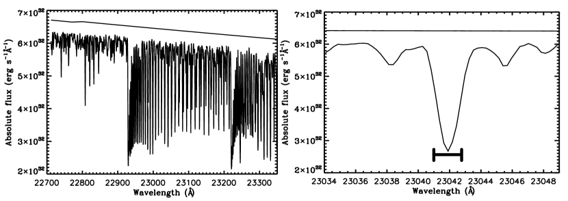
Interferometric observations done through a broad band filter blend information from the lines and continuum. Spectral resolution allows to recover much richer information, both from visibility moduli and phases. The VLTI-AMBER interferometer provides spectral resolutions of R=35, 1 500, and 12 000. In order to show the differences between these resolutions, we compute intensity maps around the CO first overtone line at 23041.75 Å (log($gf$)=-5.527 and $\chi_{ex}$=0.180 eV) for the three resolutions (Fig. 14). The resulting images are shown in the central row of the Figure, and the spectrum in the top row. The contrast, defined as in previous Section, is similar for the low and medium resolution images but it is $\sim 30\%$ lower in the high resolution image, at the CO line wavelength. Large fluctuations are seen in all lobes, but they are smaller than those seen in the H band IONIC filter (see Fig 12). The visibility fluctuations for the high spectral resolution image in the CO line are larger (second, third and fourth lobes; see dotted line in bottom panel), despite a lower intensity contrast, presumably because of the darkening of large patches of the simulated stellar surface.

Figure 14: Top row: synthetic spectrum centered on the CO first overtone band head. The left panel shows the range of wavelengths spanned by one resolution element at the VLTI-AMBER low spectral resolution of 35. The right panel shows the same for the VLTI-AMBER medium spectral resolution of 1 500, and the high spectral resolution of 12 000 (thick mark). Central row: intensity maps for those three spectral resolution elements. The intensity range is [0;$10^{5}$] erg cm^-2 s^-1 Å^-1. Bottom row: standard deviation of the visibility in the second, third and fourth lobes Solid and dashed lines correspond low and medium resolution respectively, and the dotted line to high resolution.

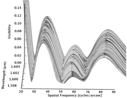
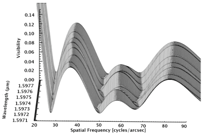
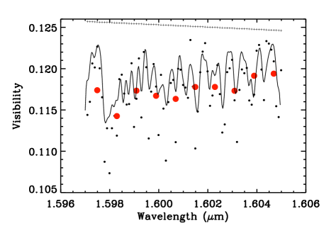
We also computed wavelength dependent visibility curves in the H band for the high and medium VLTI-AMBER resolutions. Fig. 15 displays a three-dimensional view of the visibility curves with a resolution of 12 000, and 1 500 (top panels). The simulated star has been scaled to an apparent diameter of $\sim$43.6 mas (the observed diameter of $\alpha$ Ori Perrin et al., 2004a). The displacement of the zero points with wavelength is easily seen, as well as the amplitude variations in the higher frequency lobes.

In order to mimic differential observations with an interferometer at medium and high spectral resolution, we also show in Fig. 15, the variation of the visibility modulus with wavelength for a fixed baseline (15m, i.e. in the second lobe, at $\nu=45{\rm arcsec}^{-1}$). The visibility shows variations correlated with the flux spectrum: it decreases in absorption lines. In fact, at these wavelengths wiggles and dark spots appear on intensity maps (Fig. 14, central right panel) increasing the visibility signal at frequencies higher than the second lobe. The visibility variations are much attenuated at lower spectral resolution. Observations at wavelengths in a spectral line, and in the nearby continuum will probe different atmospheric depths, and thus layers at different temperatures. They will thus provide important information on the wavelength dependence of limb darkening. Moreover, as the horizontal temperature and density fluctuations depend on the depth in the atmosphere, differential observations, with relative phase determination will provide unique constraints on the granulation pattern. The visibility variations in Fig 15, such as the steep visibility jump from 0.123 to 0.107 between 1.5975 and 1.5980 $\mu$m, could be measured in differential interferometric mode at high spectral resolution with the current precision at VLTI-AMBER (1$\%$ for visibilities of $\sim$5-10$\%$), with optimal sky conditions.

Figure 15: Top left panel: three-dimensional view of the visibility curves as a function of wavelength for a particular position angle. The spectral resolution is 12 000. Top right panel: same as in top left panel at a spectral resolution of 1 500. Bottom panel: Visibility as a function of wavelength for a baseline of $\sim$15 m, i.e. the top of the second lobe, at one particular position angle. The simulation has been scaled to an apparent diameter of $\sim$43.6 mas. The synthetic spectrum convolved to a resolution of 12 000 is over-plotted (thin solid line). The small black dots correspond to the highest resolution with AMBER (12 000), while the big red dots correspond to the medium resolution (1 500). The crosses show the uniform disk of 43.6 mas. When changing the position angle, the expected standard deviation is about 10$\%$ of the visibility (see Fig. 12).

5.5 Closure phase: departure from circular symmetry

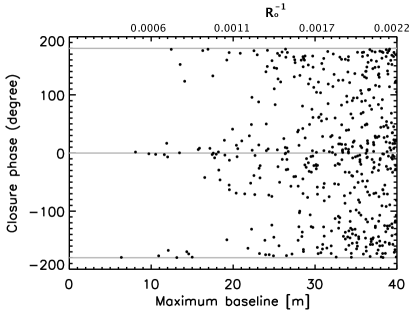
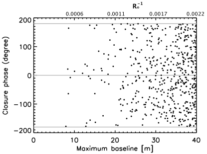
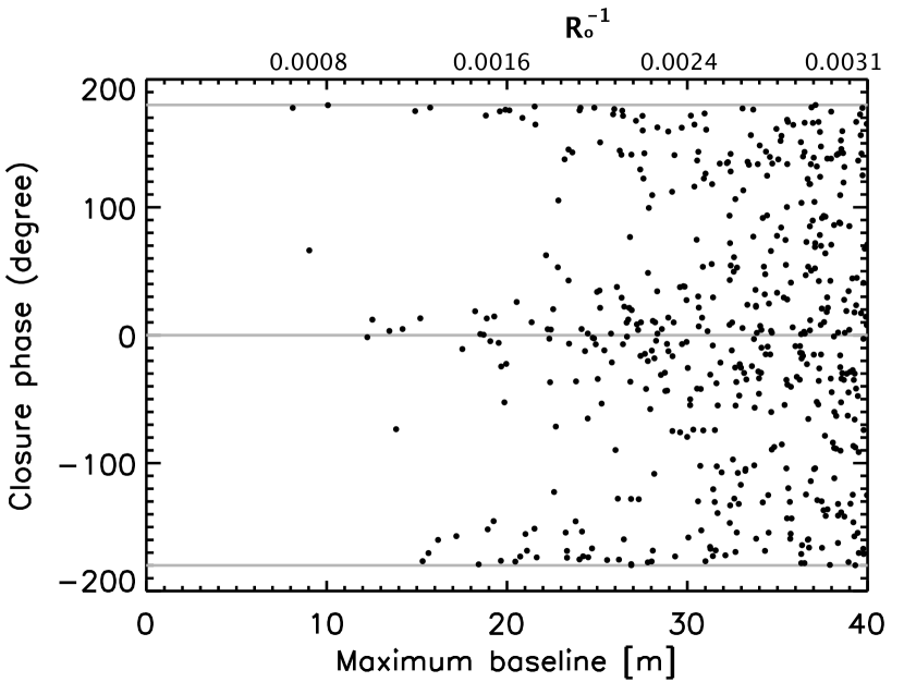
As terrestrial atmospheric turbulence affects the phases of the complex visibilities with random errors, it is impossible to derive them for individual pairs of telescopes. Instead one uses closure phase between three telescopes, as the sum of all phase differences removes the atmospheric contribution, leaving the phase information of the object visibility untouched (see e.g., Monnier, 2007). The closure phase is thus an important complementary piece of information, which can reveal asymmetries of RSG atmospheres. Fig. 16 shows the scatter plot of the closure phase of one snapshot of the RHD model computed in the IONIC filter (the scatter is similar for the K222 filter). The behavior is similar for all the snapshots. We used 500 random baseline triangles with a maximum linear extension of 40 m, and plot the closure phase as a function of the triangle maximum baseline. The closure phases deviate from zero or $\pm\pi$ already at $\sim$10 m (0.0008 R${}^{-1}_{\odot}$ if we scale the model to an apparent diameter of 43.6 mas at a distance of 174.3 pc). At higher baselines it is clearly different from zero or $\pm\pi$, values which indicate a point symmetric brightness distribution. This is a clear signature of surface inhomogenities. The characteristic size distribution on the stellar surface can also be derived from the closure phase: the contribution of small scale convection-related surface structures increases with frequency. The first deviation at $\sim$0.0008 R${}^{-1}_{\odot}$ (just beyond the first zero, see Fig. 11) corresponds to the deviation from circular symmetry of the stellar disk. It may be very efficient to constrain the level of asymmetry of RSG atmospheres by accumulating statistics on closure phase at short and long baselines, as they are easily measured with great precision. Small departure from zero will immediately reveal departure from symmetry.

Figure 16: Scatter plot of closure phases in the IONIC filter centered at 1.64 $\mu$m of 500 random baseline triangles with a maximum linear extension of 40 m. Closure phases are plotted against the longest baseline of the triangle. The upper x-axis corresponds to synthetic observations of the simulation at an apparent diameter of 43.6 mas (which corresponds to $\alpha$ Ori at a distance of 174.3 pc). The axisymmetric case is represented by the grey lines.

We also computed the closure phase for the different K band VLTI-AMBER spectral resolution intensity maps of Fig. 14. The large deviations from circular symmetry are already noticeable at low spectral resolution (Fig. 17, left panels) and the closure phase scatter do not differ much from the high spectral resolution one (right panel). This offers prospects of detecting asymmetries due to granulation without resorting to high spectral resolution.

Figure 17: Scatter plot of closure phases (cf Fig. 16 for details) obtained from the VLTI-AMBER K band low, and high spectral resolution intensity maps (Fig. 14, central left, and right panels).

6 Comparison with interferometric observations of $\alpha$ Ori

A first confrontation of our model predictions to real observations is possible for $\alpha$ Ori. We compare the synthetic visibilities derived from our RHD simulations in the continuum filter K222 (Fig. 2) with the observation of $\alpha$ Ori by Perrin et al. (2004a) that reach the third lobe in the K band. The absolute model dimensions have been scaled to match the interferometric observation in the first lobe. This corresponds to an apparent diameter of 43.6 mas at a distance of 179 pc. These values are in agreement with Perrin et al., who found a diameter of $43.64\pm 0.10$ mas, and Harper et al. (2008), who reported a distance of $197\pm 45$ pc.

We computed over 2 000 visibility curves, and we find that the data are within the visibility fluctuations due to the granulation of the simulation (Fig. 18), as already shown in Chiavassa et al., 2007. Within this large number of visibility curves, we find some that match all the observation points better than the uniform disk (with a diameter of 43.33 mas; Perrin et al., 2004a), or limb-darkened disk model (linear limb darkening law, $I\left(\mu\right)=1-a\left(1-\mu\right)$, with a diameter of 43.64 mas and $a=0.09$ also in Perrin et al.). See Fig. 18. The best match has a reduced $\chi^{2}$=0.21, and all the visibility curves fall within a $\chi^{2}$ range of [0.21,18.1]. Our RHD simulations are a great improvement over parametric models (the UD model with reduced $\chi^{2}$=19.9, and the LD model with $\chi^{2}$=22.3) for the interpretation of these interferometric observations. The observations points in the first, second, and third lobes can be reproduced with a single visibility curve, from the projection at a particular position angle of one of our snapshots (see Fig. 18). There is one observed point in the first lobe at 24.5 arcsec^-1 which is difficult to reproduce. In fact, adjustments on the absolute model dimensions of the star in order to fit this point, would lead to mismatch of the other observations at higher frequencies. However, this may be a problem with the calibration of the observation.

A more detailed comparison with $\alpha$ Ori data in the H band (Haubois et al., 2006) will be presented in a forthcoming paper (Chiavassa et al. 2009, in prep.)

Figure 18: Comparison of the RHD simulation with the $\alpha$ Ori observations (red dots with error bars) by Perrin et al. (2004a). Top panel: intensity map in the K222-FLUOR filter of the snapshot that best matches the interferometric data. The range is [0;$10^{5}$] erg cm^-2 s^-1 Å^-1. The stellar parameters of this snapshot are: $L=93\,480\,{\rm L}_{\odot}$, $R=833\,{\rm R}_{\odot}$, $T_{\rm eff}=3497$ K and $\log\leavevmode\nobreak\ g=-0.34$. The simulation has been scaled to an apparent diameter of 43.6 mas at a distance of 179 pc. The white line indicates the position angle of the projected baselines. Other panels: Synthetic visibilities from the simulation, compared with observations. Panel B) covers the whole observational range, and panels C)-E) are close-ups of the clusters of observations. The thick solid line corresponds to the best match visibility curve(reduced $\chi^{2}$=0.21). The thin solid lines show the minimum and maximum extent of variations of the visibilities. The dot-dashed, and the dashed lines are the LD, and the UD models used by Perrin et al. (reduced $\chi^{2}$=22.3, and 19.9). Note the logarithmic visibility scale.

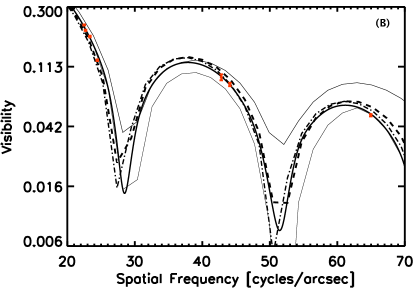
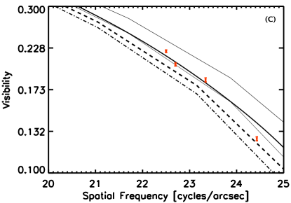
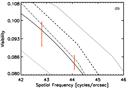
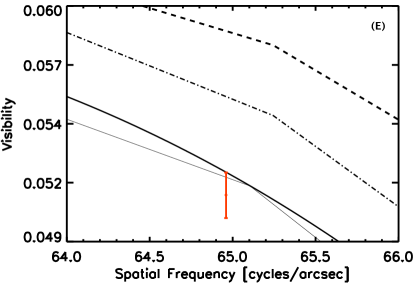
7 Conclusions

Our radiation hydrodynamics simulations confirm that only a few large granules cover the surface of RSG stars. The granules of the simulation we analyze here are 400–500 R_⊙ in diameter, and have lifetimes of years. Smaller scale structures develop and evolve within these large granules, on shorter timescales (a month).

We demonstrate that RHD simulations are necessary for a proper quantitative analysis of interferometric observations of the surface of RSGs beyond the smooth, symmetrical, limb-darkened intensity profiles. We give new average limb darkening coefficients within the H and K bands, that are significantly different from commonly used UD or LD profiles. However, these LD coefficients fluctuate with time, and the average is only indicative. Our model surface granulation causes angular and temporal variations of visibility amplitudes and phases. In the first lobe, sensitive to the radius, fluctuations can be as high as 5$\%$, and radii determinations can be affected to that extent: the radius determined with a UD fit is 3-5$\%$ smaller than the radius of the simulation, while the radius determined with a fully LD model is $1\%$ smaller.

The second, third, and fourth lobes, that carry the signature of limb-darkening, and of smaller scale structure, are very different from the simple LD case. The visibility amplitudes can be greater than the UD or LD case, and closure phases largely differ from 0 and $\pm\pi$, due to the departure from circular symmetry. The visibilities also show fluctuations with position angle, and with time, that are directly related to the granulation contrast. We also want to stress that high spectral resolution provides an extremely valuable information. The stellar surface appears dramatically different in an absorption line and in the nearby continuum, and differential observations should be easier to carry out with high precision. At lower resolution (e.g. $R=1\,500$) continuum and line information get mixed and there is a considerable loss of differential signal.

We conclude that the detection of the signature of granulation, as predicted by our simulation, is measurable with todays interferometers, if observations of both amplitude and closure phase are made at high spatial frequencies (second, third, and fourth lobes, or even further if possible). These observations will provide direct information on the time scale of variation, and of the size and contrast of granulation.

A few RSGs are prime targets for interferometry, thanks to their large diameter, proximity, and to a high infrared luminosity. Only 4 or 5 are sufficiently close and bright that imaging can be attempted, but a larger number (10-20) are within reach of less ambitious programs, like closure phase measurements.

Three approaches can be combined to characterize the granulation pattern:

• searching for angular visibility variations, observing with the same telescope configuration (covering high spatial frequencies) and using the Earth rotation in order to span 6-7 position angles in one night should be enough, if measurement errors can be kept below 10$\%$, for visibilities of the order of 5 to 10$\%$. One or two other telescope configurations would provide more frequency points, but then the change of configuration must be made within days, which is actually possible at VLTI;

• looking for temporal visibility fluctuations by observing at two (preferably more) epochs $\sim$1 month apart with the same telescope configuration. This can be easily scheduled on existing interferometer like CHARA, or the VLTI;

• looking for visibilities as a function of wavelength, at high spectral resolution, in different spectral regions belonging to spectral features and continuum. If measurement errors can be kept close to 1$\%$, for visibility of the order of $\sim$10$\%$, variations of the visibility correlated with the flux spectrum could be detected, indicating variations of the radius, of the limb-darkening, or of the granulation pattern. Such relative measurements are more easily done at the required precision than absolute visibility measurements.

These observations will bring us a wealth of information on the stars, but also on our RHD models. We know they suffer from limitations. The confrontation to observation will help us decide what approximations must be relaxed. The simulations are primarily constrained by execution time, which neccesitates several approximations, the most important ones being the limited spatial resolution and the complete lack of wavelength resolution, i.e., grey radiative transfer. This speeds up the simulations to managable execution times of several months to one year of intensive calculations for about seven years of stellar time. A higher numerical resolution shows smaller scale structures appearing within the granules that are already present in lower resolution simulations (Chiavassa et al., 2006, Fig. 10). This, however, should not affect the first few visibility lobes.

The approximation of grey radiative transfer is justified only in the stellar interior and it is not appropriate in the optically thin layers. The implementation of non-grey opacities (e.g., five wavelength groups employed to describe the wavelength dependency of the radiation field within a multigroup radiative transfer scheme, see Nordlund, 1982 for details) would be an important improvement for the hydrodynamical simulations. Ludwig et al. (1994) found for local RHD simulations that frequency dependent radiative transfer causes an intensified heat exchange of a fluid element with its environment tending to reduce the temperature differences. Consequently, the temperature fluctuations in the non-grey local models are smaller than in the grey case. This is also expected for global RSG models, and the result of such a decrease of the temperature fluctuations, would be a decreased intensity contrast and decreased visibility fluctuations.