Mean field approximation
in conformation dynamics
Abstract
We propose a new approach to the transfer operator based analysis of the conformation dynamics of molecules. It is based on a statistical independence ansatz for the eigenfunctions of the operator related to a partitioning into subsystems. Numerical tests performed on small systems show excellent qualitative agreement between mean field and exact model, at greatly reduced computational cost.
1 Introduction
Conformation transitions of molecules reflect the global spatial/temporal behaviour of the system, and in particular occur at much slower timescales compared to the elementary frequencies of the system. In a small peptide with a dozen atoms, the typical scale difference is already a factor ; for folding transitions in proteins, it ranges between and , placing these events well beyond the timescales accessible via direct trajectory simulation.
The transfer operator approach, introduced into MD by Deuflhard et al. in their fundamental paper [5] (cf. also [11, 12, 4, 6, 7, 10, 14]), allows to access long time effects through short time simulations, at the expense of needing to simulate ‘ensembles’ of initial conditions, or mathematically: to compute the evolution of densities on space. In the latter approach, dominant conformations and their transition rates can be identified via the leading eigenvalues and eigenfunctions of a suitable transfer operator. The catch is that to compute the latter, which are functions on phase resp. configuration space, the number of computational degrees of freedom of a direct discretization grows exponentially in the number of atoms.
To overcome this problem, our goal in this paper is to propose a mean field method for computing eigenstates of transfer operators, whose relationship to the exact eigenvalue problem for the transfer operator is reminiscent of that of Hartree-Fock theory to the many-particle Schroedinger equation in quantum chemistry, which overcomes an analogous ‘curse of dimension’ problem. The mean field model only has the dimensionality of a typical strongly interacting subsystem, but the densities of the different subsystems are nonlinearly coupled.
In this paper our goal is to
-
•
derive the mean field model,
-
•
validate it both by establishing exact properties and comparing to simulations of the full problem in low-dimensional examples.
The theoretical and computational results appear to us to be extremely promising. Our theoretical results include mass conservation, energy conservation, and asymptotic correctness in the limit of weak subsystem coupling (see Section 4). The numerical tests we performed on small systems show excellent qualitative agreement between mean field and exact model even when the coupling is of order one, at greatly reduced computational cost (see Section 6).
A fuller theoretical explanation of this good performance even for order one coupling would
be highly desirable, but lies beyond the scope of the present paper.
One important aspect of our simulations appears to be a careful choice of subsystems which makes at least the potential
part of the Hamiltonian non-interacting. Remarkably, such a choice is always possible
in chain molecules with a standard force field (consisting
of nearest-neighbour bond terms, third neighbour angular terms,
and fourth neighbour torsion terms), by working in inner coordinates (i.e. bond lengths,
bond angles and torsion angles). In these coordinates, subsystem coupling only occurs through
momentum exchange. But physical considerations as well as
previous work support the belief that fine details of momentum transfer do not play a decisive role in conformation dynamics:
– Molecules in solution are subject to relentless perturbations of momenta due to collisions with solvent molecules,
yet conformation dynamics robustly takes place under these conditions.
– Many of the standard models in conformation dynamics involve randomization of momenta. In the Langevin equation,
this happens by addition of white noise to the momentum equation; in the approach by Schütte in [11],
one thinks of molecular conformations as subsets of configuration space,
considers only a spatial transfer operator,
and draws momenta at random from their statistical distributions in each computational evolution step.
A more detailed analysis as well as applications of the mean field model to large systems are currently in progress and will appear elsewhere.
2 Hamiltonian dynamics and Liouville equation
In situations when quantum effects can be neglected and no bond-breaking or bond-formation takes place, the dynamics of a molecule with atoms moving about in can be described by a Hamiltonian of form
| (1) |
where , the mass matrix is a positive Matrix, and is a potential describing the atomic interactions.
In the case when all degrees of freedom are explicitly included and cartesian coordinates are used, we have (where is the number of atoms), , , and , where , , are the position, momentum, and mass of the atom. In this paper we work with the more general form (1), in which the kinetic energy is a quadratic form of depending on . This form arises when inner coordinates are used, which will play an important role below. For an -atom chain molecule, the latter consist of the nearest neighbour bondlengths , the bond angles between any three successive atoms, and the torsion angles between any four successive atoms. In order to accurately model conformation changes, will have to contain at least nearest-neighbour bond terms , third neighbour angular terms , and fourth neighbour torsion terms . In practice the potentials could either come from a suitable semi-empirical molecular force field model or from ab-initio computations.
The Hamiltonian dynamics takes the form
| (2a) | ||||
| (2b) | ||||
It will be convenient to denote the phase space coordinates by and the Hamiltonian vector field by
| (3) |
so that (2) becomes
| (4) |
The Liouville equation associated to (2) describes the transport of a passive scalar by the flow associated to eq. (2):
| (5) |
where , . Because the Hamiltonian vector field is divergence-free, eq. (5) can be written equivalently in the form
| (6) |
Since eq. (6) preserves both positivity of and the total integral , it defines an evolution on the space of probability densities
Physically it can be interpreted as an evolution equation for “ensembles” of initial data under (2). The evolution law (2) for “sharp” initial data can be recovered as a special case: is a solution to (2) if and only if the delta function transported along this solution, , is a solution to (6).
3 Molecular conformations and almost invariant sets
A conformation of a molecule – as we understand it [5, 11, 12] – is given by an almost invariant (or metastable) subset of configuration space.
Roughly speaking, an almost invariant set of a discrete dynamical system is a subset such that the invariance ratio
is close to , cf. [2]. Here denotes a suitable probability measure, typically Lebesgue measure or some -invariant measure. In our case, will be the time--map of the Hamiltonian system (2) (More generally, instead of a deterministic map, one can consider a stochastic process, cf. [2].)
Almost invariant sets can be determined via the computation of the eigenfunctions at (real) eigenvalues close to one of a certain transfer operator associated to [2, 11]. For example, the Frobenius-Perron operator
describes the evolution of measures on phase space. This is a linear operator on the space of bounded complex valued measures on . By definition, and thus the spectrum of is confined to the unit circle. Eigenmeasures at the eigenvalue are invariant measures. If is an eigenmeasure of at the eigenvalue , then
and thus for . In particular, if and are real, then there are two positive real measures such that (Hahn-Jordan decomposition). If is normalized such that is a probability measure then [2]
where and . Consequently, if is close to then both and are close to and thus almost invariant.
Transfer operators.
For measures which are absolutely continuous one can equivalently consider on . Since the flow of (2) is a volume-preserving diffeomorphism, this operator takes a particularly simple form in our case111we write in order to stress the dependence of the operator on the integration time :
| (7) |
which is the time--map of the Liouville equation (5). Note that for an arbitrary function of the Hamiltonian, the function satisfies . Thus and , normalized s.t. , is an invariant density. Of particular interest is the canonical density
| (8) |
, where and is Boltzmann’s constant. This density describes the distribution of a (constant) large number of molecules at temperature and of constant volume. Note that we can write
where and are chosen such that for each , and .
Spatial transfer operator.
As mentioned, molecular conformations should be thought of as almost invariant subsets of configuration space. Schütte [11] introduced a corresponding spatial transfer operator by averaging (7) over the momenta: Let be an invariant density of (7) with , let and consider the operator
| (9) |
where is the canonical projection onto configuration space. Schütte [11] showed that under suitable conditions, the spatial transfer operator is self-adjoint and quasi-compact on an appropriate weighted space.
Transition probabilities.
A key quantity of interest are transition probabilities from one region of space into another. The transition probability from a region into another region in phase space is given by the volume fraction of those initial data in which end up in at time ,
| (10) |
where denotes -dimensional volume. Using the expression based on the transfer operator, similarly transition probabilities between subsets of configuration space can be defined. Typically, these quantities are sought for large , but only short time simulations are numerically feasible. However, can be approximated for large by repeated matrix-vector multiplications, requiring short time evaluations of the flow only, cf. [3].
4 Mean field approximation
The problem with eq. (6) as it stands is that it is amenable to a direct numerical treatment only for very small systems, due to the exponential scaling of the number of computational degrees of freedom with particle number. If the phase space of each atom is approximated by a -point grid, such that the solution to (6) at time becomes a vector in , then the corresponding grid of the -particle system has gridpoints and the solution at time becomes a vector in . Our proposal to address this problem is partially inspired by Hartree-Fock- and density functional theory methods in quantum chemistry, which allow to overcome a related complexity problem for the -particle Schrödinger equation.
Partitioning into subsystems.
Starting point is an, for the moment arbitrary, partition of phase space coordinates into subsystem coordinates:
where is the vector of momentum coordinates corresponding to the position coordinates . Let . Then eq. (2) can be re-written as
| (11) |
Given a phase space density which depends on the phase space coordinates of all the subsystems, we introduce reduced densities for each subsystem , as follows:
| (12) |
where here and below denotes the coordinates . Note that, by the normalization of ,
that is to say the probability that the particle has some position and momentum is one. Next we calculate the exact time evolution of the subsystem densities . By (6) and (12),
Using (12) this can be rewritten in the form of a single-subsystem transport equation,
| (13) |
with underlying vector field
| (14) |
Note, however, that (13), (14) is not a closed system, since the vector field depends on the full density , not just the subsystem densities ().
Mean field model.
To close the system (13), (14), we now make the statistical independence ansatz
| (15) |
The vector field in (13) then simplifies to
| (16) |
We call the system of eqs. (13), , with given by (16) the mean field approximation to the Liouville equation. Note that it is a system of coupled nonlinear partial integrodifferential equations on the lower-dimensional subsystem phase spaces , whereas the original Liouville equation was a linear partial differential equation on , . Physically, each subsystem can be pictured, at time , as experiencing the force of the ensemble of the other subsystems in their “typical” states at time .
We record some basic properties of the mean field approximation.
-
1.
The total densities are conserved. This is immediate from the conservation law form . Thus we may assume for all and , and continue to interpret the as probability densities.
-
2.
For non-interacting subsystems, i.e.
it is exact, that is to say if the evolve via (13), (16), then the product solves the original Liouville equation (6). This follows from the fact that in this case,
and so depends only on , as a consequence of which the exact vectorfield , the reduced vectorfield in (14), and the mean field vectorfield (RHS of (16)) all coincide, regardless of the mean field ansatz (15).
-
3.
For given , , the transport equation for has the form of a Liouville equation coming from an associated time-dependent subsystem Hamiltonian,
(17) that is to say
(18) In particular, is divergence-free. Note that time-dependence of the effective subsystem Hamiltonian enters only through time-dependence of the , .
-
4.
The total energy
is conserved. To see this, calculate using the evolution equation for the and an integration by parts
But the term in square brackets equals , and hence its dot product with vanishes for all and , on account of (18); consequently .
Property 2. contains useful information regarding how the, up to now arbitrary, partitioning into subsystems should be chosen in practice. In order to maximize agreement with the full Liouville equation (5), the subsystems should be only weakly coupled. In the case of an -atom chain, this suggests to work with subsystems defined by inner, not cartesian, coordinates (as is done in the simulation of n-butane in Section 6.4 below). Namely, in inner coordinates, at least the potential energy decouples completely for standard potentials containing nearest-neighbour bond terms, third neighbour angular terms and fourth neighbour torsion terms: .
A deeper, and perhaps surprising, theoretical property of the mean field model which goes beyond property 2. concerns weakly coupled subsystems. Consider a Hamiltonian of form , where is a non-interacting Hamiltonian of the form given in 2., and is a coupling constant. It can then be shown that the exact subsystem densities obtained from (5), (12) and the mean field densities obtained by solving (13), (16) differ, up to any fixed time , only by , not the naively expected . This means that the effect of coupling between subsystems is captured correctly to leading order (in the coupling constant) by the mean field approximation. For a proof of this fact see our companion paper [8].
5 The mean field transfer operator
The mean field approximation to the Liouville equation introduced above gives rise in a natural way to a mean field approximation of the transfer operator
where is the solution to the Liouville equation (5) with initial condition . We define the mean field transfer operator as
where is the solution to the mean field approximation (13), (16), , of the Liouville equation with initial data . Note that the components of are multilinear, i.e. for fixed , the map
is linear.
The mean field spatial transfer operator.
Consider an ensemble of molecules whose distribution in phase space is given by an invariant density . We would like to describe distribution changes in the position space only (cf. Section 3). Following [11] we define the spatial transfer operator
| (19) |
where is the conditional density of for a given , i.e.
Now we define the spatial transfer operator corresponding to the mean field system. The distribution of the -th subsystem is given by
The conditional density of the for given is
We therefore define the mean field spatial transfer operator as
| (20) |
where , and
| (21) |
with , . Again, the components of are multilinear, i.e. for fixed , the map
| (22) |
is linear.
Mean field eigenfunction approximation.
Our goal is to compute eigenfunctions of the (full) spatial transfer operator (19). As approximations, we are going to use products of eigenfunctions (at the leading eigenvalues) of the linear component maps (22). In computing these, we fix to the invariant density of . This approach is motivated by the following observation for non-interacting subsystems: Let be two maps and the associated Frobenius-Perron operators. For the product map , , the Frobenius-Perron operator is given by
if . Now let and for some eigenvalues , then is an eigenvalue of with eigenfunction .
In order to compute the invariant density, we resort to an iterative procedure which is inspired by the famous Roothaan algorithm from quantum chemistry: For a given initial guess we iteratively compute a sequence , of approximate invariant densities of by computing the fixed point of each linear component map , i.e. by computing such that
6 Numerics and examples
6.1 Ulam’s method
The (spatial) transfer operator is typically considered as an operator on a (suitably weighted) ( or ) space. As such, it is not directly amenable to numerical computations. In [13], Ulam proposed the following discretization: Let be a disjoint partition of (phase or configuration) space, , where denotes the characteristic function of and the projection from onto defined by
The discretized (spatial) transfer operator is defined to be
Note that can be represented by a stochastic matrix, where the matrix entries are the transition rates between the sets and . In other words, is the probability, that , if is sampled according to a uniform distribution and then according to . This yields the numerical computation of the transition matrix by a Monte-Carlo method:
where the points are chosen i.i.d. from according to a uniform distribution, and the correspondig according to . Observe that the Markov-structure of the transfer operator is preserved: and preserve integral and positivity, and the Monte-Carlo approximation of the discretized transfer operator is a stochastic matrix, too.
Note that we have to evaluate the flow map several times for each partition element , but that these are short time simulations only. The time merely has to be large enough that motion can be observed. In particular, may be much smaller than characteristic times, e.g. for conformational changes; they can be several orders of magnitude apart. Thus, the problem of evaluating the flow at time is well conditioned, and we may use low order explicit schemes for the time integration.
6.2 Complexity
Let us first investigate the costs of setting up the discretized transfer operator for an arbitrary subsystem. Using Ulam’s method, we need to perform the following steps for each partition element :
-
•
sample and correspondingly ,
-
•
integrate the mean field system for time and initial data ,
-
•
project the endpoint onto position space and find the partition element it is contained in.
Using the canonical density for the invariant density , there is an explicit representation for the momentum distribution which can be sufficiently well approximated by a linear combination of Gaussians. The numerical time integration of the initial points requires several evaluations of the mean field vector field (18). This in turn requires the numerical evaluation of a dimensional integral. The intergal w.r.t. the can be handled analytically and by an apriori computation which is independent of the , and . Naively, this leaves us with a dimensional integral. However, note that in the case of non-interacting subsystems, i.e. , can be pulled out and the integral reduces to 1. For systems with small subsystems, i.e. and small, and in which only a fixed and small number of neighboring subsystems interact, the dimensionality of the integral is , where means all subsystems which interact with subsystem .
The solution of the resulting eigenvalue problems is simple compared with the assembling of the discretized mean field transfer operator, particularly since we are only interested in the dominant part of the spectrum. Arnoldi type iteration methods can be used.
6.3 Example: a simple 2d-system

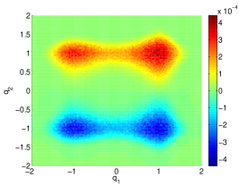
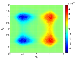
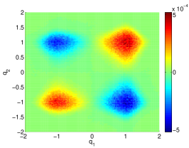
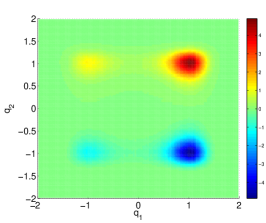
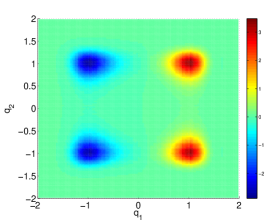
Figure 2 shows the eigenfunctions at the leading eigenvalues of the full spatial transfer operator.
The mean field approximation to the Liouville equation in this case reads explicitly
Figure 3 shows the invariant density (after ten iterations of the Roothaan type iteration) as well as the eigenfunctions and at the second eigenvalue of the two linear component maps , .
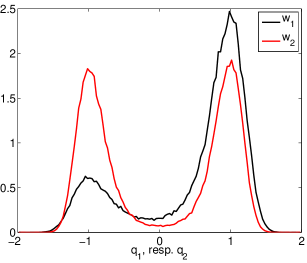
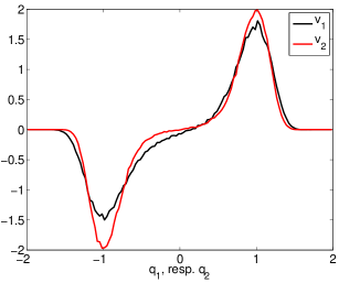
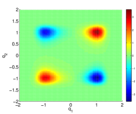
Figure 4 finally shows the functions
which serve as approximations to the eigenfunctions from Figure 2. The qualitative structure of the eigenfunctions of the full spatial operator is quite well captured.
6.4 Example: a model of n-butane
As a more realistic test case we analyse the -butane molecule CH3-CH2-CH2-CH3, cf. Figure 5.
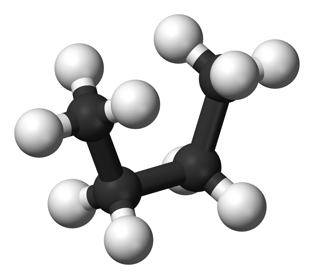
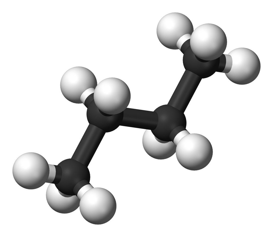
More precisely, we consider a united atom model [1] of this molecule, viewing each CH3 resp. CH2 group as a single particle. Consequently, the configuration of the model is described by six degrees of freedom: three bond lengths, two bond and one torsion angle. In order to be able to compare the results of our mean field approach to a transfer operator based conformational analysis on the full configuration space, we further simplify the model be fixing the bond lengths at their equilibrium nm. For the bond angles we use the potential
| (25) |
with and and for the torsion angle we employ
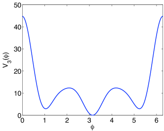
We fix g as the mass of a proton and correspondingly and as the masses of a CH2 and CH3 group, respectively. With denoting the configuration of our model, the motion of our system is determined by the Hamiltonian
| (27) |
with and the mass matrix . The latter is computed by means of a coordinate transformation to cartesian coordinates for the individual particles, assuming that there is no external influence on the molecule and its linear and angular momentum are zero: We have
and consequently
where denotes the (constant, diagonal) mass matrix of the Hamiltonian in cartesian coordinates.
Results for the full operator
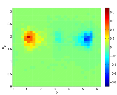
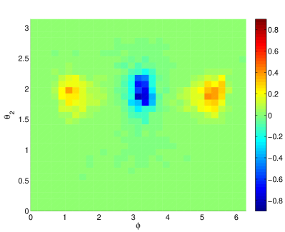
Figure 7 shows the eigenvectors of the full spatial transfer operator for system (27) at the two largest eigenvalues (computed on a grid using sample points, s integration time, realized by steps of the explicit Euler method with step size ).
Results for the mean field approach
We decompose the model into three subsystems, i.e. each configuration variable is treated separately. The Roothaan iteration is initialized with , , where is the inverse temperature corresponding to 300 K and is a corresponding normalizing factor. Figure 8 shows the mean field approximations to the two eigenvectors in Fig. 7, namely the products
where is the -factor of the invariant density of the mean field system and are the eigenvectors at the second and third largest eigenvalue of the subsystem, respectively (after ten iterations of the Roothan type iteration).
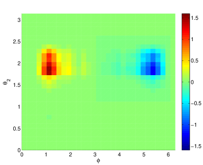
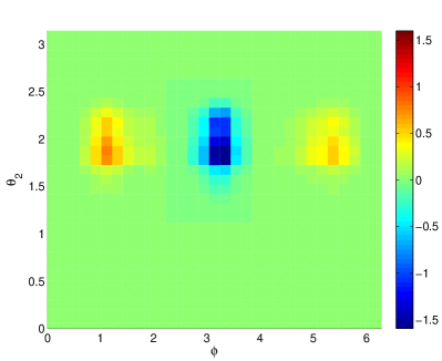
Clearly, the qualitative structure of the eigenvectors of the full operator (cf. Fig. 7) is well captured by the mean field approximation.
7 Conclusion and Outlook
We introduced a new approach to the transfer operator based conformational analysis of molecules in this paper. The central idea is a mean field approach based on a statistical independence ansatz for the eigenfunctions of the operator. The principal motivation for such an ansatz lies in its linear, as opposed to exponential, scaling of the number of computational degrees of freedom with the number of atoms, provided the subsystem size stays fixed. We established basic theoretical properties including mass and energy conservation and asymptotic correctness in the limit of weak subsystem coupling. In numerical tests on small systems, the mean field model is seen to provide a remarkably accurate representation of the true eigenfunctions. Applications to larger systems are currently in progress and will be discussed elsewhere.
8 Acknowledgements
We would like to thank Weinan E, Max Gunzburger, Mitch Luskin, and Rich Lehoucq for organizing a very stimulating Symposium on mathematical issues at the Multiscale materials modeling conference in Tallahassee, Florida, 27-31 October 2008, and for inviting us to present the work described here.
References
- [1] B. Brooks, R. Bruccoleri, B. Olafson, D. States, S. Swaminathan, and M. Karplus. CHARMM: a program for macromolecular energy, minimization, and dynamics calculations. J. Comput. Chem., 4:187–217, 1983.
- [2] M. Dellnitz and O. Junge. On the approximation of complicated dynamical behavior. SIAM J. Numer. Anal., 36(2):491–515, 1999.
- [3] M. Dellnitz, O. Junge, W. S. Koon, F. c. Lekien, M. W. Lo, J. E. Marsden, K. Padberg, R. Preis, S. D. Ross, and B. Thiere. Transport in dynamical astronomy and multibody problems. Int. J. Bifurcation Chaos Appl. Sci. Eng., 15(3):699–727, 2005.
- [4] P. Deuflhard. From molecular dynamics to conformation dynamics in drug design. In Trends in nonlinear analysis, pages 269–287. Springer, Berlin, 2003.
- [5] P. Deuflhard, M. Dellnitz, O. Junge, and C. Schütte. Computation of essential molecular dynamics by subdivision techniques. In P. Deuflhard, J. Hermans, B. Leimkuhler, A. Mark, S. Reich, and R. Skeel, editors, Computational molecular dynamics: challenges, methods, ideas, volume 4 of Lect. Notes Comput. Sci. Eng., pages 98–115. Springer, 1999.
- [6] P. Deuflhard and C. Schütte. Molecular conformation dynamics and computational drug design. In Applied mathematics entering the 21st century, pages 91–119. SIAM, Philadelphia, PA, 2004.
- [7] P. Deuflhard and M. Weber. Robust Perron cluster analysis in conformation dynamics. Linear Algebra Appl., 398:161–184, 2005.
- [8] G. Friesecke, O. Junge, and P. Koltai. Theoretical analysis of the mean field approach in conformation dynamics. In preparation, 2009.
- [9] M. Griebel, S. Knapek, and G. Zumbusch. Numerical simulation in molecular dynamics, volume 5 of Texts in Computational Science and Engineering. Springer, Berlin, 2007. Numerics, algorithms, parallelization, applications.
- [10] I. Horenko, E. Dittmer, F. Lankas, J. Maddocks, P. Metzner, and C. Schütte. Macroscopic dynamics of complex metastable systems: Theory, algorithms, and application to B-DNA. SIAM J. Appl. Dyn. Syst., to appear, 2007.
- [11] C. Schütte. Conformational dynamics: Modelling theory algorithm and applicatioconformational dynamics: Modelling, theory, algorithm, and application to biomolecules. Habilitation thesis, Free University Berlin, 1999.
- [12] C. Schütte, W. Huisinga, and P. Deuflhard. Transfer operator approach to conformational dynamics in biomolecular systems. In B. Fieder, editor, Ergodic Theory, Analysis, and Efficient Simulation of Dynamical Systems, pages 191–223. Springer, 2001.
- [13] S. M. Ulam. A Collection of Mathematical Problems. Interscience Publisher NY, 1960.
- [14] M. Weber, S. Kube, L. Walter, and P. Deuflhard. Stable computation of probability densities for metastable dynamical systems. Multiscale Model. Simul., 6(2):396–416 (electronic), 2007.