Fast search for Dirichlet process mixture models

Abstract

Dirichlet process (DP) mixture models provide a flexible Bayesian framework for density estimation. Unfortunately, their flexibility comes at a cost: inference in DP mixture models is computationally expensive, even when conjugate distributions are used. In the common case when one seeks only a maximum a posteriori assignment of data points to clusters, we show that search algorithms provide a practical alternative to expensive MCMC and variational techniques. When a true posterior sample is desired, the solution found by search can serve as a good initializer for MCMC. Experimental results show that using these techniques is it possible to apply DP mixture models to very large data sets.

1 INTRODUCTION

Dirichlet process (DP) mixture models provide a flexible Bayesian solution to nonparametric density estimation. Their flexibility derives from the fact that one need not specify a number of mixture components a priori. In practice, DP mixture models have been used for problems in genomics [Xing, Sharan, and Jordan,2004], relational learning [Xu et al.,2005], data mining [Daumé III and Marcu,2005] and vision [Sudderth et al.,2005]. Despite these successes, the flexibility of DP mixture models comes at a high computational cost. Standard algorithms based on MCMC, such as those described by [Neal,1998], are computationally expensive and can take a long time to converge to the stationary distribution. Variational techniques [Blei and Jordan,2005] are an attractive alternative, but are difficult to implement and can remain slow.

In this paper, we show that standard search algorithms, such as A*, and beam search, provide an attractive alternative to these expensive techniques. Our algorithms allows one to apply DP mixture models to very large data sets. Like variational approaches to DP mixture models, we focus on conjugate distributions from the exponential family. Unlike MCMC techniques, which can produce samples of cluster assignments from the corresponding posterior, our search-based techniques will only find an approximate MAP cluster assignment. We do not believe this to be a strong limitation: in practice, the applications cited above all use MCMC techniques to draw a sample and then simply choose from this sample the single assignment with the highest posterior probability. If one needs samples from the posterior, then the solution found by our methods could initialize MCMC.

2 DIRICHLET PROCESSES

The Dirichlet process, introduced by [Ferguson,1973], is a distribution over distributions. The DP is parameterized by a base measure $G_{0}$ and a concentration parameter $\alpha$. We write $G\textrm{~{}}\arrowvert\textrm{~{}}G_{0},\alpha\sim\mathcal{DP}(G_{0},\alpha)$ for a draw of a distribution $G$ from the Dirichlet process. We may then draw parameters $\theta_{1:N}\textrm{~{}}\arrowvert\textrm{~{}}G\sim G$. By marginalizing over $G$, we find that the draws of the parameters $\theta$ obey a Pòlya urn scheme [Blackwell and MacQueen,1973]: previously drawn values of $\theta$ have strictly positive probability of being redrawn, thus making the underlying probability measure discrete (with probability one).

By using a Dirichlet process at the top of a hierarchical model, one obtains a Dirichlet process mixture model [Antoniak,1974]. Here, one treats the $n$th parameter $\theta_{n}$ as being associated with the $n$th observation, using some likelihood function $F$. This yields the mixture model shown in Eq (1).

$$\begin{array}[]{r@{\|}l@{~\by~}l}G\textrm{~{}}\arrowvert\textrm{~{}}&\alpha,G_{0}\hfil~{}\sim~{}&\mathcal{DP}(\alpha,G_{0})\\ \theta_{n}\textrm{~{}}\arrowvert\textrm{~{}}&G\hfil~{}\sim~{}&G\\ x_{n}\textrm{~{}}\arrowvert\textrm{~{}}&\theta_{n}\hfil~{}\sim~{}&F(\theta_{n})\end{array}$$ (1)

The clustering property of the DP prefers that fewer than $N$ distinct values of $\theta$ will be used. If $K\leq N$ values are used, the $x_{n}$s can be seen to be clustered into one of $K$ clusters, determined by the $\theta$ values.

2.1 PROPERTIES

DP mixture models posses several properties that are useful for further analysis. The most basic is their well-known property of exchangeability: samples from the process are order independent. This leads to efficient MCMC techniques (see Section 2.2). An additional property of the DP that will be useful for our analysis is given as Proposition 3 by [Antoniak,1974]. He gives an explicit form for the probability of individual clusterings. In particular, suppose that a sample $x_{1},\dots,x_{N}$ is drawn from a DP mixture model as in Eq (1). At most $N$ distinct values of $\theta$ will be used (and typically far fewer). Define a vector $m_{1},\dots,m_{I}$ by: $m_{i}$ is the number of $\theta$s that appear exactly $i$ times. Thus, $N=\sum_{i}im_{i}$ and $\sum_{i}m_{i}$ is the total number of clusters. [Antoniak,1974] gives an explicit formulation for the distribution of counts $\boldsymbol{m}$:

$$P(\boldsymbol{m}\textrm{~{}}\arrowvert\textrm{~{}}\alpha,N)=\frac{N!}{\alpha^{(N)}}\frac{\alpha^{\sum_{i=1}^{I}m_{i}}}{\prod_{i=1}^{I}i^{m_{i}}(m_{i}!)}$$ (2)

where $\alpha^{(N)}$ denotes the rising factorial function: $\alpha^{(0)}=1$ and $\alpha^{(n)}=\alpha(\alpha+1)\cdots(\alpha+n-1)$.

2.2 MCMC TECHNIQUES

When the mean distribution $G_{0}$ of the DP is conjugate to the likelihood function $F$, one can analytically integrate out $G$ and the $\theta$s from Eq (1) and only maintain a vector of cluster assignments, $\boldsymbol{c}_{1:N}$. The vector $\boldsymbol{c}$ serves to specify which $x_{n}$s were generated from the same mixture component $\theta$, so that $x_{n}$ is drawn according to $F(\theta_{c_{n}})$. Using the exchangeability of the DP, a single Gibbs iteration proceeds as follows [Neal,1998, Algorithm 3]. For each $n$, we draw $c_{n}$ to be a new cluster with probability proportional to $\alpha H(x_{n})$ and draw it equal to an existing cluster $d$ with probability $N_{-n,d}H(x_{n}\textrm{~{}}\arrowvert\textrm{~{}}\{x_{i}\textrm{~{}}\arrowvert\textrm{~{}}c_{i}=d,i\neq n\})$. Here, $\alpha$ is the concentration parameter for the DP, $N_{-n,d}$ is the number of elements of $\boldsymbol{c}$ (other than $n$ itself) that are equal to $d$. Finally, $H(x\textrm{~{}}\arrowvert\textrm{~{}}S)$ is the posterior probability of $x$ given that $S$ has been observed, Eq (3).

$$H(x\textrm{~{}}\arrowvert\textrm{~{}}S) \triangleq\int\textrm{d}G_{0}(\theta\textrm{~{}}\arrowvert\textrm{~{}}S)F(x\textrm{~{}}\arrowvert\textrm{~{}}\theta)$$ (3)

$$=\frac{\int\textrm{d}G_{0}(\theta)F(x\textrm{~{}}\arrowvert\textrm{~{}}\theta)\prod_{y\in S}F(y\textrm{~{}}\arrowvert\textrm{~{}}\theta)}{\int\textrm{d}G_{0}(\theta)\prod_{y\in S}F(y\textrm{~{}}\arrowvert\textrm{~{}}\theta)}$$

By analogy, we will also write $H(\boldsymbol{x}_{1:N}\textrm{~{}}\arrowvert\textrm{~{}}S)$ to denote the marginal posterior probability of $N$ data points. In general, when working in the exponential family, $H$ will be available in closed form and thus the Gibbs sampling is efficient.

[Jain and Neal,2004] propose a Metropolis-Hastings sampler based on splitting and merging existing clusters. This algorithm is shown to mix faster than the vanilla Gibbs sampler outlined above. It works by first randomly choosing two data points. If the data points are currently in different clusters, a proposal is created that merges the two clusters. If the data points are currently in the same cluster, a proposal is generated the splits the cluster. [Jain and Neal,2004] present three variants on this idea. In the first variant, splits are determined completely randomly. In the second variant, a small Gibbs sampler is run to determine the splits. In the third variant, a Gibbs sampler is run to determine the splits and the Metropolis-Hastings iterations are interleaved with the standard Gibbs iterations described above.

3 SEARCH

MCMC is an attractive technique for inference in DP mixture models. However, in many real-world cases, one does not actually need a sample of cluster assignments from the posterior, but actually seeks only a single cluster assignment. In these cases, a sample is extracted from an MCMC run and a single cluster assignment—the MAP assignment—is extracted from the sample. This raises the question: is Gibbs sampling a good search algorithm? We show experimentally (see Section 4.1) that it is often not.

function DPSearch input: a scoring function $g$, beam size $b$, data $\boldsymbol{x}_{1:N}$ output: a clustering $\boldsymbol{c}$ 1:  initialize max-queue: $Q\leftarrow[\langle\rangle]$ 2:  while $Q$ is not empty do 3:     remove state $\boldsymbol{c}_{1:N^{0}}$ from the front of $Q$ 4:     if $N^{0}=N$ then return $\boldsymbol{c}$ 5:     for all clusters $d$ in $\boldsymbol{c}$ and a new cluster do 6:        let $\boldsymbol{c}^{0}=\boldsymbol{c}\oplus\langle d\rangle$ 7:        compute the score $s=g(\boldsymbol{c}^{0},\boldsymbol{x})$ 8:        update queue: $Q\leftarrow$ Enqueue($Q$, $\boldsymbol{c}^{0}$, $s$) 9:     end for 10:     if $b$ $<\infty$ and $\left|Q\right|>b$ then 11:        Shrink queue: $Q\leftarrow Q_{1:b}$ 12:          (drop lowest-scoring elements) 13:     end if 14:  end while

Figure 1: The generic DP search algorithm.

In general, it will be intractable to find the exact MAP solution, as doing so is NP-hard (by reduction to graph partitioning). Here, we describe a set of possible search algorithms one can apply to DP mixture models for finding the true MAP solution for small problems or an approximate MAP solution for large problems. The generic search algorithm we use is shown in Figure 1. It takes an ordered set of data points $\boldsymbol{x}_{1:N}$, a scoring function and a maximum beam size. It maintains a max-queue of clusterings of prefixes. In each iteration, it removes the most promising element $\boldsymbol{c}$ from the queue and expands it by a single data point. The two elements of variability in the algorithm are the scoring function and the maximum beam size.

The search algorithm is guaranteed to find the maximum a posteriori clustering if the beam size is $\infty$ and the scoring function is admissible. In words, $g$ should over-estimate the probability of the best possible clustering $\boldsymbol{c}$ that agrees with $\boldsymbol{c}^{0}$ on the first $N^{0}=\left|\boldsymbol{c}^{0}\right|$ elements. In equations, we write $\boldsymbol{c}\upharpoonright N^{0}$ to denote the restriction of $\boldsymbol{c}$ to the first $N^{0}$ elements. Thus:

$$g(\boldsymbol{c}^{0},\boldsymbol{x})\geq\max_{\boldsymbol{c}:\boldsymbol{c}\upharpoonright N^{0}=\boldsymbol{c}^{0}}p(\boldsymbol{c},\boldsymbol{x})$$ (4)

We further require that when $\left|\boldsymbol{c}\right|=\left|\boldsymbol{x}\right|$, equality holds.

However, for efficiency, it is useful to use scoring functions $g$ that occasionally underestimate the true posterior probability. While these functions no longer guarantee that the exact MAP solution will be found, they are often more efficient because $g$ can be tighter, even if it is not a strict upper bound (see Section 4.1 for supporting evidence).

The posterior probability $p(\boldsymbol{c},\boldsymbol{x})$ can be factored as $p(\boldsymbol{c})p(\boldsymbol{x}\textrm{~{}}\arrowvert\textrm{~{}}\boldsymbol{c})$. Here, the probability of a cluster vector $p(\boldsymbol{c})$ is given in Eq (2) (the mapping from the $\boldsymbol{c}$ vector to the $\boldsymbol{m}$ vector is straightforward). The probability of the data given the clusters is given in Eq (5).

$$p(\boldsymbol{x}\textrm{~{}}\arrowvert\textrm{~{}}\boldsymbol{c})=\prod_{d\in\boldsymbol{c}}H(\boldsymbol{x}_{\boldsymbol{c}=d})$$ (5)

Here, we write $\boldsymbol{x}_{\boldsymbol{c}=d}$ as shorthand for $\{x_{n}:c_{n}=d\}$. Our goal is a function $g(\boldsymbol{c}^{0},\boldsymbol{x})$ that upper bounds the probability of the best clustering $\boldsymbol{c}$ that completes $\boldsymbol{c}^{0}$, as in Eq (5). For brevity, we write $N^{0}$ to be the length of $\boldsymbol{c}^{0}$ and $K^{0}$ to be the number of clusters in $\boldsymbol{c}^{0}$.

An upper bound can be obtained by independently upper-bounding the two terms, $p(\boldsymbol{c})$ and $p(\boldsymbol{x}\textrm{~{}}\arrowvert\textrm{~{}}\boldsymbol{c})$. In fact, we do not upper bound $p(\boldsymbol{c})$ but rather explicitly maximize it. The algorithm for this computation is given in Section 3.1. The maximization of $p(\boldsymbol{x}\textrm{~{}}\arrowvert\textrm{~{}}\boldsymbol{c})$ is more complex and cannot be performed explicitly. We give three techniques for this maximization. The first, trivial computation, is admissible but very loose (Section 3.2). The second is tighter but still admissible (Section 3.3). The third is tighter yet, but is no longer admissible (Section 3.4).

Matlab code for solving these problems is available online at http://hal3.name/DPsearch/.

3.1 MAXIMIZING THE CLUSTERS

It is possible to explicitly compute the clustering $\boldsymbol{c}$, beginning with $\boldsymbol{c}^{0}$, that maximizes the posterior cluster probability given in Eq (2). Consider the case of adding a single data point to $\boldsymbol{m}$. (Recall that $m_{i}$ denotes the number of clusters that contain exactly $i$ data points.) If this new data point corresponds to a new cluster, then $m_{1}$ will increase by one. If this data point corresponds to an existing cluster that already contains $\ell$ data points, then $m_{\ell}$ will decrease by one and $m_{\ell+1}$ will increase by one. This gives a change in probability for adding a new data point in Eq (6).

$$\rightarrow\textrm{new}:\frac{\alpha}{m_{1}+1}~{}~{}~{}~{}~{}\rightarrow\ell:\frac{\ell}{\ell+1}\frac{m_{\ell}}{m_{\ell+1}+1}$$ (6)

By the exchangeability of the underlying process, we obtain exchangeability on the $\boldsymbol{m}$ vector. Thus we can greedily search for completions of an initial $\boldsymbol{m}^{0}$ by executing one of the two actions in Eq (6) for the remaining $N-N^{0}-1$ data points. In particular, for $N-N^{0}-1$ steps, we find the value of $\ell$ (or “new”) that maximizes Eq (6) and modify the corresponding locations in the vector. After all steps, we simply compute the probability of the $\boldsymbol{m}$ vector according to Eq (2).

When $N$ is very large, the loop for computing the optimal $\boldsymbol{m}$ can be time-consuming. One can greatly accelerate the computation by noticing that once the largest cluster gets sufficiently large, it will simply continue to grow for the remainder of the iterations. Specifically, if in any step the largest cluster is increased from size $\ell-1$ to $\ell$, and $[\ell m_{\ell}]/[(\ell+1)(m_{\ell+1}+1)]$ dominates $\alpha/[m_{1}+1]$, then one can stop the search process and simply further increase $\ell$ with all remaining elements. Additionally, it is helpful to cache previously computed values for repeated use.

3.2 A TRIVIAL FUNCTION

Given a clustering $\boldsymbol{c}^{0}$ of the first $N^{0}$ elements, we can trivially upper bound $p(\boldsymbol{x}\textrm{~{}}\arrowvert\textrm{~{}}\boldsymbol{c})$ from Eq (5) by considering only the first $N^{0}$ data points. For this admissible scoring function, we use Eq (7).

$$g_{\textrm{Trivial}}(\boldsymbol{x}\textrm{~{}}\arrowvert\textrm{~{}}\boldsymbol{c}^{0})\triangleq\prod_{k\in\boldsymbol{c}^{0}}H(\boldsymbol{x}_{\boldsymbol{c}^{0}=k})$$ (7)

Using the trivial scoring function is essentially equivalent to just using a path cost with a zero heuristic function in standard A* search. As such, we expect this scoring function will lead to an inefficient search.

3.3 A TIGHTER FUNCTION

The inefficiency of the trivial scoring function given in Section 3.2 is due to the fact that it does not take into account any of the unclustered data points. We can obtain a tighter scoring function by accounting for the probability of the as yet unclustered data points. We do this by simplifying the maximization as follows.

$$\max_{\begin{subarray}{c}\boldsymbol{c}:\\ \boldsymbol{c}\upharpoonright N^{0}=\boldsymbol{c}^{0}\end{subarray}}p(\boldsymbol{x}\textrm{~{}}\arrowvert\textrm{~{}}\boldsymbol{c})$$

$$= \max_{\begin{subarray}{c}\boldsymbol{c}:\\ \boldsymbol{c}\upharpoonright N^{0}=\boldsymbol{c}^{0}\end{subarray}}\prod_{k\in\boldsymbol{c}}H(\boldsymbol{x}_{\boldsymbol{c}=k})$$ (8)

$$= \max_{\begin{subarray}{c}\boldsymbol{c}:\\ \boldsymbol{c}\upharpoonright N^{0}=\boldsymbol{c}^{0}\end{subarray}}\prod_{n=1}^{N}H(x_{n}\textrm{~{}}\arrowvert\textrm{~{}}\boldsymbol{x}_{\boldsymbol{c}_{1:n-1}=c_{m}})$$ (9)

$$= \prod_{n=1}^{N^{0}}H(x_{n}\textrm{~{}}\arrowvert\textrm{~{}}\boldsymbol{x}_{\boldsymbol{c}^{0}_{1:n-1}=c_{m}})$$ (10)

$$~{}~{}~{}~{}~{}~{}~{}~{}~{}~{}~{}~{}\max_{\begin{subarray}{c}\boldsymbol{c}:\\ \boldsymbol{c}\upharpoonright N^{0}=\boldsymbol{c}^{0}\end{subarray}}\prod_{n=N^{0}+1}^{N}H(x_{n}\textrm{~{}}\arrowvert\textrm{~{}}\boldsymbol{x}_{\boldsymbol{c}_{1:n-1}=c_{m}})$$

$$\leq g_{\textrm{Trivial}}(\boldsymbol{x}\textrm{~{}}\arrowvert\textrm{~{}}\boldsymbol{c}^{0})$$ (11)

$$\prod_{n=N^{0}+1}^{N}\max_{1\leq k\leq K^{0}+1}\max_{\begin{subarray}{c}\boldsymbol{c}:\\ \boldsymbol{c}\upharpoonright N^{0}=\boldsymbol{c}^{0}\\ c_{n}=k\end{subarray}}H(x_{n}\textrm{~{}}\arrowvert\textrm{~{}}\boldsymbol{x}_{\boldsymbol{c}_{1:n-1}=c_{m}})$$

The key idea for this scoring function is to treat each as-yet unclustered data point independently. In particular, for some $n>N^{0}$, we know that it will either fall into one of the $K$ clusters that exist in $\boldsymbol{c}^{0}$, or it will fall into a new cluster. So, for each unclustered point $x_{n}$, we choose a value $k$ for which cluster it falls in to. We then must cluster all remaining points $x_{N^{0}+1}\dots x_{n-1}$ as to only whether they fall into cluster $k$.

Despite the fact that this latter maximization is simpler, it is still not tractable (effectively because $H(x\textrm{~{}}\arrowvert\textrm{~{}}S)$ is not monotonic in $S$, even for the exponential family). The solution we propose is to replace each remaining $x_{m}$ ($N^{0}<m<n$) with a replica of $x_{n}$. In this way, we do obtain monotonicity of $H$ and may simply keep adding replicas of $x_{n}$ to $S$ so long as this increases the cluster probability.

3.4 AN INADMISSIBLE FUNCTION

The foregoing scoring functions are attractive because they provably lead to optimal clusterings. However, this optimality comes are a price: the NP-hardness of the search problem implies that they will often be inefficient. This inefficiency comes from their lack of tightness. Here, we give a very simple scoring function that is significantly tighter, and therefore leads to much faster clusterings. Unfortunately, this heuristic is no longer admissible and therefore the search is no longer guaranteed to find the globally optimal solution. The function we use is given in Eq (12).

$$g_{\textrm{Inad}}(\boldsymbol{x}\textrm{~{}}\arrowvert\textrm{~{}}\boldsymbol{c}^{0})\triangleq g_{\textrm{Trivial}}(\boldsymbol{x}\textrm{~{}}\arrowvert\textrm{~{}}\boldsymbol{c}^{0})\prod_{n=N^{0}+1}^{N}H(x_{n})$$ (12)

This scoring function uses the true probability of the existing clusters and then assigns each new data point to a new cluster. This is inadmissible because, for example, if the last two data points are identical, it would be preferable to cluster them together.

When using this scoring function, the order in which the data points is presented becomes important. We have found that a useful heuristic is to order the data points by increasing marginal likelihood. This is likely because examples with high marginal likelihood are more likely to be in their own clusters anyway, and hence the heuristic is better. (See Section 4.3 for some experiments comparing ordering strategies.)

4 EXPERIMENTAL RESULTS

We present results on three problems, one based on artificial data, one based on the MNIST images data set and one based on the NIPS papers data set. All experiments were run on a $3.8$GHz Intel Pentium 4 machine with $4$Gb of RAM.

4.1 ARTIFICIAL DATA

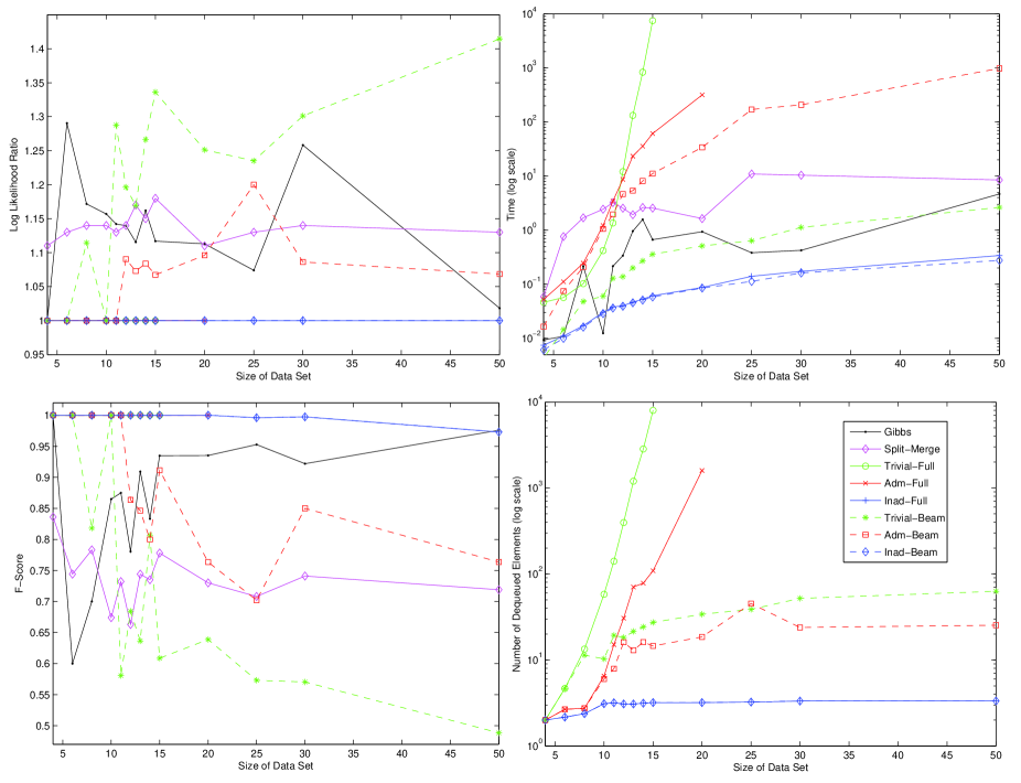
Figure 2: Results on artificial data set; x-axis is always the size of the data set. (UL) y-axis is the ration of the data negative log likelihood to the data negative log likelihood found by exhaustive search (lower is better); (BL) y-axis is f-score (higher is better); (UR) y-axis is computation time in seconds (lower is better); (BR) y-axis is number of elements enqueued during search (lower is better).

Our first set of experiments are on artificial data to demonstrate the scaling properties of the search methods and to compare them directly to Gibbs sampling. For these problems, we generate a data set according to a Gaussian/Gaussian DP mixture model with prior mean zero and prior variance $10$. We generate data sets of increasing size ($N\in\{4,6,8,10,11,12,13,14,15,20,25,30,50\}$). We first run Gibbs sampling and split-merge on each data set. We then run six search algorithms. The first three search algorithms run full search using the three scoring functions described above. The last three search algorithms use the three scoring functions described above, but with a maximum queue size of $10$. For each data set size, we generate $10$ data sets and average results across these.

Comparison between a sampling approach and a non-sampling approach is difficult. We perform our comparison to be as unfair to our proposed approach as possible: i.e., we try to make sampling look as good as possible. We run both samplers as follows. We do fifteen runs of the sampler for 1000 iterations each. The first five are initialized with a single cluster; the second five are initialized with $N$ clusters; the last five are initialized randomly with $\log N$ clusters. For each run, there will be a sample that achieves the highest log likelihood. We choose this iteration as the stopping point. The best of the best log likelihoods over the 15 runs is then reported as the final score. The time reported is the time it took to get to that log likelihood in the single run. That is, the numbers reported are overly optimistic in terms of time, and in line with practice in terms of performance. For the split-merge algorithm [Jain and Neal,2004], we only use the third variant that performs intermediate Gibbs sampling. The other split-merge algorithms fared surprisingly poorly—often losing significantly even to standard Gibbs in terms of log likelihood.

The results of these experiments are shown in Figure 2. The upper-left graph shows a plot of the data negative log likelihood as a function of data set size (lower is better). The negative log likelihoods are presented as a ratio to the log likelihood of the true MAP assignment. Interestingly, both inadmissible search algorithms achieve optimal performance. The beam-based admissible heuristics do worse, and the Gibbs sampler never reaches optimal performance (except on the smallest data set). The split-merge performance is quite variable: sometimes better than Gibbs, sometimes worse.

In the upper-right graph, we plot computation time as a function of data set size. Split-merge is almost always slightly slower than Gibbs. As can be easily seen, the time taken for both admissible heuristics grows quite fast and, at least for the trivial heuristic, becomes intractable after only 10-15 data points. The Trivial-Beam remains reasonably efficient (on par with Gibbs), but also had the worst negative log likelihood performance. The Admissible-Beam is actually reasonably slow because the computation of the heuristic is time-consuming. As expected, the inadmissible heuristic (with or without beam) is always the fastest.

The bottom-left graph shows the f-score (geometric mean of precision and recall) of pair-wise “same cluster or not” decisions for the clustering found by the different algorithms against the ground truth (higher is better). As we can see, the inadmissible heuristic always performs best, while the others vary significantly in performance (Gibbs, for some reason, does quite poorly initially but then improves as the size of the data set increases).

Finally, the bottom-right graph shows (for only the search-based algorithms) the number of states enqueued during search. This corresponds roughly with the upper-right graph (time) but excludes considerations such as the time to compute the heuristic. As expected, the inadmissible heuristic enqueues by far the fewest entries (in fact, for most of these algorithms, the number of elements dequeued by the inadmissible heuristic was between $N$ and $N+5$ for all algorithms, meaning that pure greedy search may be reasonable).

4.2 HANDWRITTEN DATA

For this experiment, we use the handwritten data set from MNIST (specifically, the version assembled by Sam Roweis) consisting of images of numbers (in $28\times 28=784$ dimensions). Following [Kurihara, Welling, and Vlassis,2006], we preprocess the data by centering and spherizing it, then running PCA to obtain a $50$-dimensional representation. This data set consists of $60,000$ images, and thus only the inadmissible heuristic is sufficiently efficient to run (we use a beam of 100, though this turns out to be unnecessarily large). We run on three versions of the data: a $5\%$ subset, a $20\%$ subset and the full set. In all cases, we use $\alpha=1$ and a prior variance of $0.1$.

At the $5\%$ level, search completes in just over $11$ seconds, roughly $270$ data points per second. The algorithm finds a solution using $11$ clusters and achieves a negative log likelihood of $2.04e5$. Running Gibbs on this data set takes roughly $40$ seconds per iteration, and after $100$ iterations achieves a best performance of $2.09e5$. Split-merge obtains a log-likelihood of $2.05e5$, but takes almost two hours to do so. At the $20\%$ level, search completes in just over $105$ seconds ($115$ elements per second) with a final negative log likelihood of $8.02e5$ (and 21 clusters). Gibbs sampling takes roughly $18$ minutes per iteration and find a best solution of $8.34e5$ (after $100$ iterations). Split-merge obtains a solution with negative log likelihood of $8.15e5$ after eight hours. Finally, for the full data set, search completes in just under $15$ minutes (roughly $66$ data points per second) with a score of $3.96e6$ (and 27 clusters). Gibbs takes an egregious $7$ hours per iteration on this data, so we were only able to run $15$ iterations, leading to a best score of $4.2e6$. Split-merge was also to slow to run for more than $15$ iterations, achieving a score of $4.1e6$ after about $7$ days.

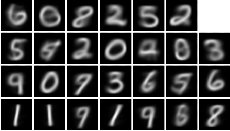
Figure 3: Mean images for clusters found on the full ($60k$ examples) MNIST data set.

In Figure 3, we show the mean image from each cluster found by the search algorithm on the full data set (sorted by cluster size). Qualitatively, these clusters appear quite reasonable. ([Kurihara, Welling, and Vlassis,2006] present a similar figure for variational techniques; however, their model uses a full Gaussian/inverse-Wishart prior while ours only uses a Gaussian and we use a fixed prior variance. One could easily adapt our algorithms to use the full prior, but we do not do so in the experiments reported here.)

4.3 NIPS DOCUMENTS

Finally, to demonstrate the applicability of our algorithm to discrete data, we apply the same model to the set of papers from NIPS 1–12 (assembled by Sam Roweis). This data set consists of $1740$ documents over a vocabulary of roughly $13k$ words. In our model, we drop the top ten words from the vocabulary and retain only the top 1000 from the remainder. For this data, we use the Dirichlet/Multinomial DP mixture model with $\alpha=1$ and a symmetric Dirichlet prior with parameter equal to $10$.

training hidden units error learning weight generalization network weights regression layer algorithm recurrent gradient nodes prediction theorem convergence node student
spike neuron neurons cells synaptic firing cell cortical cortex activity synapses stimulus excitatory orientation inhibitory membrane spikes ocular dominance fig
mixture speech em likelihood image tangent hmm clustering word images pca recognition posterior bayesian speaker gaussian experts kernel cluster classification
chip circuit analog motion image voltage vlsi visual auditory images velocity sound retina intensity optical pulse disparity template pixel silicon
policy reinforcement state controller action control actions robot reward agent mdp learning states sutton policies trajectory planning singh barto rl
object objects units views face image hidden unit visual images recognition attractor activation faces features layer attention feature representations module
bounds threshold polynomial bound theorem depth boolean proof gates lemma dimension tree node concept clause class functions winnow boosting maass
motion head motor visual eeg eye direction subjects stimulus ica movements cells movement cortex velocity cue field parietal vor spatial
word classifiers classifier hmm rbf character recognition training speech mlp characters hybrid user context net hidden layer trained words error
belief evidence similarity posterior bayesian retrieval user propagation hypotheses query concept approximation examples exact images iii image mackay database nodes

Table 1: Most indicative words for each of the ten largest clusters (out of fourteen) of documents from NIPS papers. Sorted by cluster size.

Running DP search (with the inadmissible heuristic) on this data set takes roughly $21$ seconds ($83$ documents per second) and results in fourteen clusters. For each cluster, we extract the top twenty words from the documents assigned to that cluster (“top” as determined by tf-idf score). These are depicted in Table 1 (sorted by cluster size).

We also experiment with alternative orderings of the data set for this problem. When the data is presented in ascending order of marginal likelihood, the resulting log likelihood is $2.4407e6$. When this order is reversed, the resulting log likelihood is $2.4740e6$. Finally, we consider presentations in random order. Over ten such orders, the mean log likelihood is $2.4489e6$ and the variance is $0.0067e6$. (Of all the random passes, only one achieves a higher log likelihood than the default ascending order, and does so with a small gain: $2.4403e6$.) This suggests that the ascending order is a reasonable heuristic.

In comparison the vanilla Gibbs sampling and the split-merge proposals, the search algorithm again performs significantly better. The log likelihood for the best Gibbs clustering on this data was $3.2e6$ and for the split-merge proposals it as $3.0e6$, both taking a little over an hour.

5 PRIOR WORK

Although in this paper we have only compared our search-based technique to straightforward Gibbs sampling, there are other inference techniques for DP mixture models. Still within the context of MCMC, [Xing, Sharan, and Jordan,2004] propose a Metropolis-Hastings sampler that is shown to mix faster than the Gibbs sampler and is only moderately more challenging to implement. An alternative, recent proposal for inference in DP mixture models is to make use of particle filters (sequential MCMC) [Fearnhead,2004]. Particle filters look somewhat like a stochastic beam search algorithm and, as such, are similar in spirit to the approach proposed here.

We are additionally aware of two deterministic approaches to inference in DP mixture models based on variational techniques. The first, due to [Blei and Jordan,2005], employs the stick-breaking construction for the Dirichlet process [Sethuraman,1994] to construct a finite variational distribution for the infinite mixture model. On artificial data, they report on the order of a $100-300$ decrease in time (over Gibbs sampling) with essentially identical held-out data log likelihoods. Very recently, [Kurihara, Welling, and Vlassis,2006] present even more efficient variational algorithm for DP mixture models. In contrast to the method of [Blei and Jordan,2005], the new algorithm employs an infinite variational distribution and a collapsed distribution [Kurihara, Welling, and Teh,2007]. It can be further accelerated (at least in the Gaussian case) by using kd-trees for caching sufficient statistics of the data set.

6 CONCLUSIONS

We have presented an algorithm for finding the MAP clustering for data under a Dirichlet Process mixture model, a task that appears regularly in many practical applications. It has been shown to be extremely efficient (clustering a data set of $60k$ elements in under $15$ minutes in Matlab) and general (we have shown applications both to continuous and discrete data sets). Moreover, for small data sets, we have shown relatively efficient schemes for finding provably optimal solutions to the MAP problem. Our results, especially with the inadmissible scoring function, show that one can obtain a very good approximate MAP solution incredibly quickly. Profiling shows that our main bottleneck is actually optimizing $p(\boldsymbol{c})$ from Section 3.1, not $p(\boldsymbol{x}\textrm{~{}}\arrowvert\textrm{~{}}\boldsymbol{c})$. In the worst case, this optimization is quadratic in the size of the data set, not linear. We are currently investigating ways of making this more efficient.

In comparison to variational approaches to DP mixture models [Blei and Jordan,2005, Kurihara, Welling, and Vlassis,2006], our algorithm is applicable to exactly the same data (exponential family with conjugate priors) and suffers from the same drawback: one cannot easily re-estimate the concentration parameter. However, given the speed of our algorithm, one could easily use multiple runs with Bayesian model selection to find a suitable value. It should be noted that the results presented in papers discussing variational approaches compare to Gibbs sampling in terms of log likelihood and speed. The general result is that the variational approaches obtain similar log likelihoods about $100-300$ times faster. Our results with the inadmissible function show that we can often achieve better results to Gibbs. It is difficult to imagine an algorithm that is more computationally efficient than search with our inadmissible function.

The primary advantage of MCMC techniques over our method is that they produce a true representation of the posterior, provided that they are run for long enough However, if a true sample of the posterior is desired, it would be natural to run our algorithm as an initializer for any MCMC algorithm. This would yield the benefits of a sample from the posterior without requiring that the sampler first find a region of high posterior probability. Additionally, MCMC techniques can be applied to non-conjugate distributions (at least in theory) by using an embedded sampling procedure to estimate the intractable integrals. One could, in principle, use the same methodology within our search framework, though this would obviate many of the speed benefits. An alternative would be to use an efficient deterministic approximation.

Acknowledgments.

Thanks to Andy Carlson and the three anonymous reviewers whose constructive criticism and pointers helped improve this paper.

References

- [Antoniak,1974] Antoniak, Charles E. 1974. Mixtures of Dirichlet processes with applications to Bayesian nonparametric problems. The Annals of Statistics, 2(6):1152–1174, November.
- [Blackwell and MacQueen,1973] Blackwell, David and James B. MacQueen. 1973. Ferguson distributions via Pòlya urn schemes. The Annals of Statistics, 1(2):353–355, March.
- [Blei and Jordan,2005] Blei, David and Michael I. Jordan. 2005. Variational inference for Dirichlet process mixtures. Bayesian Analysis, 1(1):121–144, August.
- [Daumé III and Marcu,2005] Daumé III, Hal and Daniel Marcu. 2005. A Bayesian model for supervised clustering with the Dirichlet process prior. Journal of Machine Learning Research, 6:1551–1577, September.
- [Fearnhead,2004] Fearnhead, Paul. 2004. Particle filters for mixture models with an unknown number of components. Journal of Statistics and Computing, 14:11–21.
- [Ferguson,1973] Ferguson, Thomas S. 1973. A Bayesian analysis of some nonparametric problems. The Annals of Statistics, 1(2):209–230, March.
- [Jain and Neal,2004] Jain, Sonia and Radford M. Neal. 2004. A split-merge Markov Chain Monte Carlo procedure for the Dirichlet process mixture model. Journal of Computational and Graphical Statistics, 13:158–182.
- [Kurihara, Welling, and Teh,2007] Kurihara, Kenichi, Max Welling, and Yee Whye Teh. 2007. Collapsed variational dirichlet process mixture models. In Proceedings of the International Joint Conference on Artificial Intelligence (IJCAI).
- [Kurihara, Welling, and Vlassis,2006] Kurihara, Kenichi, Max Welling, and Nikos Vlassis. 2006. Accelerated variational DP mixture models. In Advances in Neural Information Processing Systems (NIPS).
- [Neal,1998] Neal, Radford M. 1998. Markov chain sampling methods for Dirichlet process mixture models. Technical Report 9815, University of Toronto, Department of Statistics and Department of Computer Science, September.
- [Sethuraman,1994] Sethuraman, Jayaram. 1994. A constructive definition of Dirichlet priors. Statistica Sinica, 4:639–650.
- [Sudderth et al.,2005] Sudderth, Erik, Antonio Torralba, William Freeman, and Alan Willsky. 2005. Describing visual scenes using transformed Dirichlet processes. In Advances in Neural Information Processing Systems (NIPS).
- [Xing, Sharan, and Jordan,2004] Xing, Eric P., Roded Sharan, and Michael I. Jordan. 2004. Bayesian haplotype inference via the Dirichlet process. In Proceedings of the International Conference on Machine Learning (ICML).
- [Xu et al.,2005] Xu, Zhao, Volker Tresp, Kai Yu, Shipeng Yu, and Hans-Peter Kriegel. 2005. Dirichlet enhanced relational learning. In Proceedings of the International Conference on Machine Learning (ICML).