Hot stars and interferometry

Abstract

What is long-baseline optical/IR stellar interferometry? A few years ago, many astronomers might not have been able to answer that question properly. This is today hopefully not the case anymore, because mainstream facilities, such as the VLTI, the Keck-I or the CHARA array, offer now this delicate technique to an astronomer who wants to observe his favourite object at the highest angular resolution available. The large teaching effort on what is interferometry and for what purpose it can be used, together with weak, but already convincing imaging capabilities, make the technique reaching a “mature” state. I will not discuss here the details of the technique, as already many booklets are now published on the subject, but rather describe what makes long-baseline stellar interferometry attractive for the field of hot star astrophysics.

Stars: general

0.1 What do we measure with an interferometer?

Long-baseline optical/IR interferometry measurements are often exclusively considered to be the so-called “visibility” measurement. We need to come back to what this “visibility” is linked to, to understand that it is not the only measurement made available by interferometers. The visibility is related to the so-called spatial coherence function of light, well described in e.g. Haniff (2007); Millour (2008). This coherence function is proportional to the Fourier-transform of the space-distribution of light from the observed object.

What is often called “visibility” is in fact the normalized amplitude of this Fourier-transform. However, a proper definition of “visibility” contains both the amplitude and the phase of this coherence function, and we will see that the phase contains also interesting information for the observation of a hot star.

0.1.1 Visibility

“Visibility”, i.e. the “normalised-amplitude-of-the-Fourier-transform-of-the-space-distribution-of-light-of-an-observed-object” in its common accepted definition, is a number between zero and one. The bigger the object is at a given baseline and wavelength, the lower the visibility is. In the same way, for a given object and wavelength, the bigger the baseline is, the lower the visibility will be. That is why it is often used as a probe of the typical angular size of an object.

On the other hand, the behaviour along wavelength will be somewhat more complicated. As an example, H-band is commonly more sensitive to stellar photosphere, whereas N-band will probe more dusty structures, which are commonly much larger than the stars. The visibility may increase, or decrease with larger wavelength, whether there is a dusty envelope around a star or not. Therefore, the wavelength-dependent behaviour of the visibility is not straightforward and will highly depend on the nature of the object observed.

0.1.2 Phases

Absolute phase measurements with optical interferometry are either very difficult or impossible to achieve due to the Earth’s atmosphere blurring. Therefore, very often, the only available phase measurements are partial, through the closure phase and/or the differential phase.

0.1.3 Closure phase

Closure phase is a phase measurement made available when combining three telescopes in a triangle. Its main advantage is that it is mostly insensitive to any atmospheric effect. Its main drawback is that it measure 1/3 of the whole phase information out of the three baselines available. It is commonly accepted as a probe for “asymmetry” of the object when it is non-zero. However an object can be asymmetric and exhibit a zero closure phase for a given baseline and a given wavelength. Hence a zero closure phase is not always a sign of the object being symmetric. As a summary, closure phase is a tool to probe for asymmetric structures, such as inhomogeneities in circumstellar disks Meilland et al. (2007a), or in the stellar photosphere itself (Domiciano de Souza et al., 2008).

0.1.4 Differential phase

Differential phase is the wavelength-dependent variation of the phase that can be partially reconstructed out of the interferometric measurements, as soon as there is a spectrograph inhere. It provide invaluable phase information as it still contains the wavelength-dependency of the phases in e.g. an emission line (Meilland et al., 2007b), at the cost of loosing the absolute (average) level of the phase on the whole wavelength-range considered. Hence, it is possible to probe the change of asymmetry of an object as a function of wavelength with such a measure (Millour et al., 2007).

0.2 What is the angular size of a massive hot star?

The question how to measure the size of stars has been raised by Fizeau (1851), which induced a series of unsuccessful observations, made by Stephan (1874), and led to an upper limit on the size of stars. It has been only when larger instruments became available that the first star, Betelgeuse, could be resolved by Michelson & Pease (1921). However, until the reborn of interferometry by Labeyrie (1975), only very few stars could have their angular diameters measured. The question whether one can measure the angular size of hot stars with the modern technique of interferometry covers in fact two issues, which are to resolve the stellar photosphere itself, and to resolve the circumstellar envelope or wind, which are sometimes the dominant source of emission at some specific wavelengths.

0.2.1 B-type stars

B-type massive stars have usually a very small angular diameter. This is due to the fact that main-sequence stars have small physical sizes, but can be found close to us, and that giant or supergiant stars are bigger in physical sizes, but are sparser in the Galaxy and hence far away from Earth. An example of such is the closest Be star, $\alpha$ Arae, which has a radius of 4.8R_⊙ and is located at 74 pc from the Earth. Converted in angular diameter, this gives a diameter of 0.6 mas, which is slightly above the capacities in resolution for the VLTI. On the other hand, the disk-like envelope of this star was measured by AMBER to be $\simeq$4 mas in radius, which is well within the possibilities of the VLTI.

A (highly non-exhaustive) list of Be stars and B[e] supergiant stars, observed up to now, is presented in table 1, and shows that for the brightest and closest high mass B-type stars, the stellar photosphere itself is always smaller than 1 mas. On the other hand, the envelope sizes of these stars range from less than 1 mas for the smallest one up to $\approx$10 mas for the largest ones, making possible to image some of them with the current capabilities of the interferometers. This also explains why most of the interferometric studies on massive B-type stars have focused on their circumstellar envelopes and not really on their stellar disk itself.

3      Name      Star ø      Envelope ø      Reference      (mas)      (mas)      B-type stars      $\kappa$ CMa      [0.24]      11      Meilland et al. (2007a)      MWC 297      [0.22]      10      Malbet et al. (2007)      $\alpha$ Arae      [0.6]      8      Meilland et al. (2007b)      HD87643      -      4      Millour et al. (In preparation.)      CPD-52^∘2874      -      3.4      Domiciano de Souza et al. (2007)      $\zeta$ Tau      0.4-[0.5]      2      Gies et al. (2007); Carciofi et al. (2009)      $\kappa$ Dra      0.39      1.72      Gies et al. (2007)      $\delta$ Cen      [0.45]      1.6      Meilland et al. (2008)      $\gamma$ Cas      0.5      1.36      Gies et al. (2007)      $\phi$ Per      0.3      0.51      Gies et al. (2007)      O-type stars      Rigel ($\beta$ Ori)      [2.43]      -      Richichi et al. (2005)      O star of $\gamma^{2}$ Vel      [0.48]      -      Millour et al. (2007)      $\theta^{1}$ Ori C      [0.22]      -      Menten et al. (2007); Simón-Díaz et al. (2006)      WRs, LBVs, etc.      WR star of $\gamma$ Vel      -      [0.3-0.6]      Millour et al. (2007)      $\eta$ Car      -      2.2-3.8      Weigelt et al. (2007)

Table 1: A non-exhaustive list of hot stars observed with interferometry (in near-infrared) and their measured [or estimated] sizes.

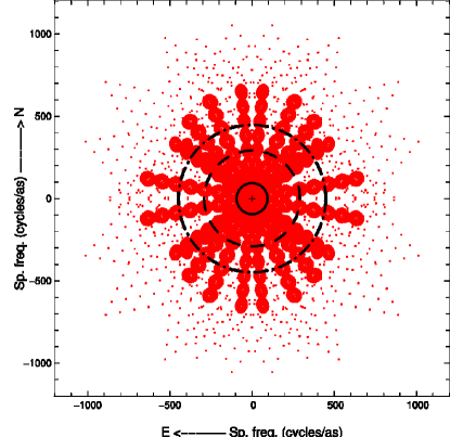
Figure 1: A sketch of the perfect interferometer: it would combine the extreme collecting area of the E-ELT with large baselines, with a set of fixed auxilliary telescopes (ATs), made e.g. using the same segments as in the E-ELT. High fidelity images at an angular resolution of 0.45 mas in K band may be reconstructed in this configuration with only 3 different hour angles ($\approx$3 h of observing time, see UV map on the right). The center circle show the UV frequencies probed by the E-ELT alone, the dashed circle show the same for the VLTI (130 m maximum baseline) and the dash-dotted circle represent the maximum reachable baseline of the VLTI (200 m), with an upgrade of its delay lines.

0.2.2 O-type stars

Among the regions where one can find massive O-type stars, the Orion nebula is maybe one of the closest places, with a distance of $414\pm 7$ pc (Menten et al., 2007). The young B- and O-type stars of the Orion trapezium, and especially $\theta^{1}$ Ori C, are at the origin of the ionization of the famous nebula itself. If one take the expected radius for such a star ($R_{*}=9.9R_{\odot}$ Simón-Díaz et al., 2006), this gives an angular diameter of 0.22 mas. A similar estimate (0.15 mas) can also be found in the CADARS catalog of stellar angular diameters (Pasinetti Fracassini et al., 2001). Other O-type stars are listed in table 1 showing that only Rigel ($\beta$ Ori), which has an angular diameter of 2.43 mas (Richichi et al., 2005), can be resolved with current facilities. This means that very long baselines combined with shorter wavelengths are needed to resolve these stars or their close-by co-rotating wind features (only a few $R_{*}$).

0.2.3 Wolf-Rayet and other exotic-types stars

Wolf-Rayet stars are evolved massive stars, thought to be progenitors of supernovae. They are among the hottest stars with temperatures $\approx$70,000 K and no direct information on the underlying star can be obtained with spectroscopy as its fast ($v_{\infty}\approx 1500-2000$ km$\times$s^-1) and dense wind completely veils the star. Therefore, fundamental parameters such as their luminosity and mass can be accessed through complex radiative transfer models, extensively tested with spectroscopy, but that still need to be checked by direct measurements. Interferometry allows to resolve the line forming regions and probe the models. Also, some WR stars exhibit a large and dusty circumstellar shell that can be probed with interferometry (Millour et al., 2009). Angular diameters of WR stars and their wind are very small (see Table 1), therefore, only circumstellar features are today reachable with interferometry. For LBV stars, the situation is slightly better since their wind is denser and, hence, appear larger.

0.3 Bigger and larger interferometers for the future?

The today’s interferometric facilities have fairly bright limiting magnitudes compared to single dish telescopes. Both the VLTI and Keck-I have extreme limiting magnitudes lying in the 10-11 mag range in the K-band (Kishimoto, Weigelt, private communication). At these limits, expected relative uncertainties will be larger than 10%, which would not be suitable to resolve fainter (and hence smaller) hot stars. More conservative limiting magnitudes ($K=7$ for VLTI with UTs, $K=5$ for VLTI with ATs) are usually adopted. One has to note that the V band limit has also to be taken into account ($V\leq 13.5$ for the VLTI). As an illustration, the reachable number of Wolf-Rayet stars with the offered VLTI performances is about 10.

Another limitation of current facilities is the fact that current baselines are limited to few hundred meters, still making stellar surfaces resolution above the current capacities, as explained in the previous sections. One cannot combine today at the same time large baselines (like in the CHARA array) and large collecting areas (like in the VLTI and the Keck-I).

Having limiting magnitudes fainter than e.g. 15 in K combined with baselines larger than e.g. 300 m would increase the number of potential targets for a given object class from few dozens to many thousands, allowing one to access the statistical aspect of hot stars astrophysics. This might be reached with a combination of higher-throughput facilities and instruments, the generalization of dual field interferometry, and of course larger collectig areas and larger baselines lengths. Sketch of such future facilities have been already described (Labeyrie et al., 1988; Riaud et al., 2001; Vakili et al., 2003), but they all combine relatively small apertures (D$\approx$2 m). Accessing fainter magnitudes might be reached by combining ELTs with interferometry. This might be done via a set of fixed auxilliary telescopes dispatched around an ELT. A sketch of such is shown in Fig. 1.

Q. & A. during the conference:

1. How many stars were oberved with interferometers up to now?

2. This largely depends on the type of objects considered. In total, few thousand stars are reachable with current facilities. $\approx$1500 targets were observed with the VLTI. The raw data can be accessed through the ESO archive for all stars, after a proprietary time of one year. There is also a PTI and Keck-I archive.

3. What future for VLTI in the E-ELT era?

4. The large difference in collecting area (VLTI$\ll$E-ELT) as well as angular resolution (VLTI$\gg$E-ELT) make these two facilities complementary.

References

- Carciofi et al. (2009) Carciofi, A. C., et al. 2009, A&A, In press.
- Domiciano de Souza et al. (2008) Domiciano de Souza, A., et al. 2008, A&A, 489, L5
- Domiciano de Souza et al. (2007) Domiciano de Souza, A. et al. 2007, A&A, 464, 81
- Fizeau (1851) Fizeau, H. 1851, Sur un moyen de déduire les diamètres des étoiles de certains phénomènes d’interférence
- Gies et al. (2007) Gies, D. R., et al. 2007, ApJ, 654, 527
- Haniff (2007) Haniff, C. 2007, New Astronomy Review, 51, 565
- Labeyrie (1975) Labeyrie, A. 1975, ApJ, 196, L71
- Labeyrie et al. (1988) Labeyrie, A., et al. 1988, in ESO Astrophysics Symposia, 29, 669–693
- Malbet et al. (2007) Malbet, F., et al. 2007, A&A, 464, 43
- Meilland et al. (2007a) Meilland, A., et al. 2007a, A&A, 464, 73
- Meilland et al. (2008) Meilland, A., et al. 2008, A&A, 488, L67
- Meilland et al. (2007b) Meilland, A., et al. 2007b, A&A, 464, 59
- Menten et al. (2007) Menten, K. M., et al. 2007, A&A, 474, 515
- Michelson & Pease (1921) Michelson, A. A. & Pease, F. G. 1921, ApJ, 53, 249
- Millour et al. (In preparation.) Millour et al. In preparation., A&A
- Millour (2008) Millour, F. 2008, New Astronomy Review, 52, 177
- Millour et al. (2009) Millour, F., et al. 2009, The Messenger, 135, 26
- Millour et al. (2007) Millour, F., et al. 2007, A&A, 464, 107
- Pasinetti Fracassini et al. (2001) Pasinetti Fracassini, L. E., et al. 2001, A&A, 367, 521
- Riaud et al. (2001) Riaud, P., et al. 2001, Liege International Astrophysical Colloquia, 85–95
- Richichi et al. (2005) Richichi, A., et al. 2005, A&A, 431, 773
- Simón-Díaz et al. (2006) Simón-Díaz, S., et al. 2006, A&A, 448, 351
- Stephan (1874) Stephan, E. 1874, in C. R. Acad. Sci., Vol. 78, 1008
- Vakili et al. (2003) Vakili, F., et al. 2003, SF2A, 365
- Weigelt et al. (2007) Weigelt, G., 2007, et al. A&A, 464, 87