Tunneling times with covariant measurements

Abstract

We consider the time delay of massive, non-relativistic, one-dimensional particles due to a tunneling potential. In this setting the well-known Hartman effect asserts that often the sub-ensemble of particles going through the tunnel seems to cross the tunnel region instantaneously. An obstacle to the utilization of this effect for getting faster signals is the exponential damping by the tunnel, so there seems to be a trade-off between speedup and intensity. In this paper we prove that this trade-off is never in favor of faster signals: the probability for a signal to reach its destination before some deadline is always reduced by the tunnel, for arbitrary incoming states, arbitrary positive and compactly supported tunnel potentials, and arbitrary detectors. More specifically, we show this for several different ways to define “the same incoming state” and ”the same detector” when comparing the settings with and without tunnel potential. The arrival time measurements are expressed in the time-covariant approach, but we also allow the detection to be a localization measurement at a later time.

PACS: 03.65.Db, 03.65.Nk

I Introduction

Questions related to the tunneling phenomenon have been actively studied since the early days of quantum mechanics, and some of them are still not resolved. In the simple case of a massive particle moving in one dimension through a localized (tunnel) potential, the question of the ”time spent in the tunnel” is especially interesting, and has given rise to extensive discussion (see e.g. Hartman ; Kijowski ; Enders ; Steinberg ; Chiao ; Nimtz and the references therein). Some difficulties in dealing with this problem are rooted in the absence of a selfadjoint ”time operator” (“Pauli’s Theorem” Pauli ). Instead, one has to use more general framework of positive operator measures (POMs) Ludwig ; Holevo ; Werner ; Busch . For a survey on time in quantum mechanics, see Muga .

An old observation related to tunneling times is the so called Hartman effect Hartman , which states that the transmitted part of a wave function appears to move faster through the tunnel than the corresponding free state. More precisely, after a long rectangular barrier and for a wave function of narrow momentum distribution, in leading order the transmitted pulse appears at the end of the tunnel instantaneously. Therefore, it has been suggested that this effect means superluminal signal transport Enders ; Nimtz . However, all this is only true for the shape of the wave function disregarding normalization. But obviously, especially for long tunnels, for which the gain in speed would only be noticeable, the transmission probability is exponentially small. So in any attempt to utilize the Hartman effect for a faster signal transmission, we would have to analyze the trade-off between transmission probability and transmission speed.

The main result of this paper is that this trade-off is always trivial: when damping is taken into account, transmission through a tunnel will always slow down the signal. Figures 1 and 2 show a sketch of the result of an arrival time measurement in a possible situation: The arrival time probability density for the transmitted particles peaks earlier than for the free particles. The density may even become larger at some times. But if we look at the integrated density, i.e., the probability for the particles to arrive before a given deadline $t$, plotted here as a function of $t$, then the free particles win.

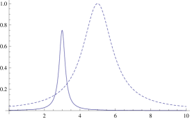
Figure 1: Arrival probability density for free (dashed line) and transmitted (solid line) particles

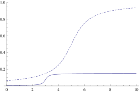
Figure 2: Probability for arrival up to time t for free (dashed line) and transmitted (solid line) particles

This is true in remarkable generality: for any incoming state, any tunnel potential, and any detector. It is even true for several, in general inequivalent approaches to formalizing the rules of this race. Indeed we need to choose a precise notion of arrival detection, of the equality of initial wave functions, and of the equality of detectors for tunneling and free dynamics. The equality of initial states is a non-trivial issue, because the two states are subject to different dynamical evolutions. So at least we need to fix a reference time. For this we have two choices, namely either a fixed time (set to zero by convention), or $t=-\infty$, i.e., asymptotic equality of the incoming states in the sense of scattering theory. In this case we fix the direction from which the particles are coming by choosing input states with positive momentum.

On the detection side, a natural choice is to describe the detectors as covariant arrival time observables Holevo ; Werner . Again this raises the issue of how to compare the two cases, because the covariance condition explicitly depends on the time evolution, and an observable can be covariant with respect to only one of them. Again scattering theory helps, by defining a bijective correspondence between the respective sets of covariant observables: we identify observables, which give the same probability distributions on states coinciding for $t\to+\infty$. This identification is also natural for including finer descriptions of the detection process. For example, we could modify both time evolutions by including an imaginary “optical” potential, resulting in contraction semigroups rather than unitary groups. The loss of normalization is then interpreted as arrival probability. Even more realistically, we could model the detector by a system in a bound state, interacting with the particle through a potential, and getting ionized in the detection process. The ionization time (as measured by a covariant observable on the escaping electron) is then taken as the detection time. It will be shown elsewhere how these ideas lead to special cases of covariant measurements.

In this paper we also look at another way of setting up the finish line for the race: For particles traveling in the positive $x$-direction, any time $t$, and any position $a$ behind (=to the right of) the tunnel, we can replace the event ”the particle has arrived at point $a$ before time $t$” by “the particle is located in the half axis $[a,\infty)$ at time $t$”. The latter statement requires only a position measurement, and hence does not require the theory of arrival times. Although the two statements are not equivalent, and correspond to different effect operators (the first probability is, by definition, increasing as a function of $t$, but the second is not in general increasing), they will be qualitatively similar, and equal in the classical limit. Note that both the arrival times and the localization observables (see e.g. Ali ; Busch ) are represented by positive operator measures, constrained by a covariance condition. In order to emphasize the analogy with arrival times, for which a projective measurement does not exist, we also allow localization observables, which are general positive operator measures (“POM”), rather than just the standard position observable.

To summarize, we are looking at the following three approaches to our problem:

	approach	initial reference time	detection
I	covariant time	$-\infty$	time-covariant
II	localization	$-\infty$	localization
III	time-zero	$0$	localization

The combination of the time-zero initialization with time-covariant measurements is conspicuously absent from this table, because the identification of detectors under different dynamics requires asymptotic scattering theory, which we wanted to avoid in this setting.

There would be more possibilities for the detection, with more realistic detector descriptions, and some of these are now under investigation. Approaches I and II have been discussed in a recent paper by Werner and Ruschhaupt (to be published, see also a conference report by Werner at the 40th Toruń Symposium, June 2008). Here we have added the ”time zero approach”, as well as formulated the treatment in a way that brings the use of positive operator measures and covariance to the front.

II Preliminaries and notations

As mentioned in the introduction, we have three distinct approaches, each formulated in terms of covariant positive operator measures. Because of the covariance property (which we will precisely define shortly below), the mathematical structure of the problem will be the same in each case, once the observable is suitably transformed. More specifically, time observables are defined via time translations and localization observables via space translations; in both cases, the structure is the same in the Hilbert space where the translation generator acts multiplicatively. Accordingly, we will transform into the ”energy representation” $L^{2}([0,\infty),dE)$ for the arrival time case, and into the ”momentum space” $L^{2}(\mathbb{R},dk)$ for the other two cases. Notationally, this is conveniently implemented by defining the relevant basic operators (multiplication in particular) in the generic $L^{2}(\mathbb{R})$, and this is done in the following.

II.1 Basic notations

For any Hilbert space $\mathcal{H}$, we let $\mathcal{L}(\mathcal{H})$ denote the set of bounded operators on $\mathcal{H}$. Let $M$ be the multiplication operator acting in $L^{2}(\mathbb{R})$ as $(M\varphi)(x)=x\varphi(x)$, on its domain of selfadjointness. Let $D$ be the differential operator $i\frac{d}{dx}$, likewise in $L^{2}(\mathbb{R})$. These operators will be used in different forms: in the ”position representation” $L^{2}(\mathbb{R},dx)$, we will put $Q:=M$ and $P:=-D$; they are the standard position and momentum operators. In the ”momentum representation” $L^{2}(\mathbb{R},dk)$, the multiplication operator $M$ represents momentum, and in the ”energy representation” $L^{2}([0,\infty),dE)$ it acts as ”multiplication by energy”.

Let $F\in\mathcal{L}(L^{2}(\mathbb{R}))$ be the Fourier-Plancherel operator, i.e. the unitary operator with

$$(F\varphi)(y):=\frac{1}{\sqrt{2\pi}}\int_{\mathbb{R}}e^{-iyx}\varphi(x)\,dx,\ \ \varphi\in L^{2}(\mathbb{R})\cap L^{1}(\mathbb{R}).$$

The operators $M$ and $D$ are well-known to be connected via the operator equalities

$$D=FMF^{*}=-F^{*}MF.$$ (1)

(See e.g. (Akhiezer, , pp. 106, 112); it will be crucial to get the signs correctly.) We will also denote $\hat{\psi}=F\psi$, and $\check{\psi}=F^{*}\psi$, for $\psi\in L^{2}(\mathbb{R})$. For any operator $A$ in $L^{2}(\mathbb{R})$ (bounded or not), we denote $\hat{A}:=FAF^{*}$, and $\check{A}=F^{*}AF$.

In the physical context, we use the Fourier operator $F$ in the natural way as $F:L^{2}(\mathbb{R},dx)\to L^{2}(\mathbb{R},dk)$, so that the notations $\hat{\psi}$, $\check{\psi}$ are as usual. Also the meaning of $\hat{A}$ and $\check{A}$ should be clear: if $A$ is an operator in the position space, then $\hat{A}$ is the corresponding operator in the momentum space, and if $A$ acts in the momentum space, then $\check{A}$ is how it acts in the position space. In particular, $\hat{Q}=D$ acts as a differential operator in $L^{2}(\mathbb{R},dk)$, while $\hat{P}=M$ is the multiplication.

For any Borel function $f:\mathbb{R}\to\mathbb{C}$, the operator $f(M)$, as defined via the spectral calculus, is simply the multiplication by $f$, on its domain $\left\{\varphi\in L^{2}(\mathbb{R})\mid\int|f(x)\varphi(x)|^{2}\,dx<\infty\right\}$. We let $P_{+}=\chi_{[0,\infty)}(M)$ and $P_{-}=\chi_{(-\infty,0]}(M)$ (where $\chi_{X}$ is the characteristic function of a set $X\subset\mathbb{R}$). Then $P_{\pm}\in\mathcal{L}(L^{2}(\mathbb{R}))$ are projections, and we do the obvious identifications $P_{+}L^{2}(\mathbb{R})=L^{2}([0,\infty))$, $P_{-}L^{2}(\mathbb{R})=L^{2}((-\infty,0])$. Using the above defined notation, we have $\check{P}_{\pm}=F^{*}P_{\pm}F$. Since $F^{2}$ is the parity operator, we also have $\check{P}_{\mp}=I-\check{P}_{\pm}=FP_{\pm}F^{*}=\hat{P}_{\pm}$.

The reason for introducing these projections is that we will frequently need the subspaces of positive and negative momenta. In $L^{2}(\mathbb{R},dk)$, these are just $P_{+}L^{2}(\mathbb{R},dk)=L^{2}([0,\infty),dk)$ and $P_{-}L^{2}(\mathbb{R},dk)=L^{2}((-\infty,0],dk)$, while in the position space $L^{2}(\mathbb{R},dx)$, they are the images of the projections $\check{P}_{\pm}$.

II.2 Covariant observables

Each of the three approaches is formulated in terms of positive operator measures, defined on the Borel $\sigma$-algebra $\mathcal{B}(\mathbb{R})$ of the real line. We proceed to define this concept.

Let $\mathcal{H}$ be a Hilbert space. A set function $E:\mathcal{B}(\mathbb{R})\to\mathcal{L}(\mathcal{H})$ is said to be a positive operator measure (POM) if $E$ is strongly (or, equivalently, weakly) $\sigma$-additive, and $0\leq E(B)\leq I$ for all $B\in\mathcal{B}(\mathbb{R})$. For any pair of vectors $\varphi,\psi\in\mathcal{H}$, and a POM $E:\mathcal{B}(\mathbb{R})\to\mathcal{L}(\mathcal{H})$ we can associate the complex measure $B\mapsto E_{\psi,\varphi}(B):=\langle\psi|E(B)\varphi\rangle$.

A POM will also be called observable, when a quantum system is associated with the Hilbert space $\mathcal{H}$. The physical meaning of this is imported by postulating that for any state operator $\rho$ (i.e. a positive operator of trace one), the number ${\rm Tr}[\rho E(B)]$ is the probability that the measurement of $E$ yields a value from the Borel set $B$, given that the system is prepared into the state $\rho$. Note that here we do not require an observable to be normalized in the sense that $E(\mathbb{R})=I$. The positive operator $I-E(\mathbb{R})$ is simply interpreted as corresponding to the event of ”no detection”.

We will need two kinds of observables, arrival time and localization observables. In the first case the problem of time in quantum mechanics is obviously involved. Without delving into the long history of this question (see the references given in the introduction), we recall that the use of POMs is forced by the fact that there is no selfadjoint operator giving eligible ”time” probability distributions.

A time observable associated with the free evolution $H_{0}:=P^{2}$ is a POM $E:\mathcal{B}(\mathbb{R})\to\mathcal{L}(L^{2}(\mathbb{R},dx))$ satisfying the covariance condition

$$e^{itH_{0}}E(B)e^{-itH_{0}}=E(B+t),\ \ \text{for all }B\in\mathcal{B}(\mathbb{R}),\,t\in\mathbb{R}.$$ (2)

This encodes the minimal requirement that the measurement of $E$ performed at time $t>0$ gives a result from the range $[t_{1},t_{2}]$ with the same probability as the measurement of $E$ at $t=0$ gives a result from the shifted range $[t_{1}+t,t_{2}+t]$.

For an arrival time observable, we additionally require that $E(\mathbb{R})$ is the projection onto the subspace of positive momenta, i.e. $E(\mathbb{R})=\check{P}_{+}$. This is simply because the ”arrivals” are supposed to be coming only from the left, so the negative momentum part is not detected (see Werner for a more general formulation of screen observables.)

In the second (and third) approach, we need localization observables. The standard localization observable is given by the spectral measure $E^{Q}$ of the position operator $Q$. However, in order to emphasize the mathematical similarity of the approaches, we consider general localization observables, i.e. POMs $E:\mathcal{B}(\mathbb{R})\to\mathcal{L}(L^{2}(\mathbb{R},dx))$, satisfying translation covariance and velocity boost invariance:

$$e^{-itP}E(B)e^{itP} =E(B+t), e^{itQ}E(B)e^{-itQ} =E(B),\ \ \text{ for all }~t\in\mathbb{R}.$$ (3)

Such observables have been studied in the context of approximate (or imprecise) position measurements (see e.g. Davies ; Ali ; Busch ; Carmeli ). In particular, they are all known to be of the form $E=\mu*E^{Q}$, where $\mu:\mathcal{B}(\mathbb{R})\to\mathcal{L}(\mathcal{H})$ is a probability measure, and the convolution is defined in terms of the associated complex measures.

II.3 The tunnel potential and scattering in one dimension

Having defined the covariance concepts, we move on consider the tunnel potential. Quite naturally, the essential quantity will turn out to be the transmission amplitude associated with the scattering from the potential. The relevant information will be given in Theorem 1 below.

Let $H_{0}:=P^{2}$ be the free Hamiltonian (in the position representation). For our purposes, a tunnel potential is a (measurable) function $V:\mathbb{R}\to\mathbb{R}$ such that

• $V$ is compactly supported and bounded;

• The Hamiltonian $H=H_{0}+V$ has no eigenvalues (e.g. $V$ is positive).

Condition (i) assures that the tunnel is strictly localized in some interval $(x_{0},x_{1})$, and does not form an impenetrable barrier. The second condition means that it actually acts as a barrier rather than e.g. a well. In order to not to exclude the square barriers typically used in the context of tunneling, we have not required continuity for the potential.

Next we need to recall some basic facts of scattering theory in one dimension. Under the above conditions defining the tunnel potential, the Hamiltonian $H=H_{0}+V$ is selfadjoint, with purely absolutely continuous spectrum $[0,\infty)$. In particular, there are no bound states. The wave operators

$$\Omega_{\pm}=s-\lim_{t\rightarrow\pm\infty}e^{itH}e^{-itH_{0}}$$

exist and asymptotic completeness holds, i.e. $\Omega_{+}(\mathcal{H})=\Omega_{-}(\mathcal{H})=L^{2}(\mathbb{R},dx)$. The operators $\Omega_{\pm}$ are unitary, and the unitary operator $S=\Omega_{-}^{*}\Omega$, which connects incoming and outgoing asymptotics, is called the scattering operator. We have the following intertwining relations.

$$e^{-itH}\Omega_{\pm} =\Omega_{\pm}e^{-itH_{0}}, t\in\mathbb{R};$$ (4)

$$e^{-itH_{0}}S =Se^{-itH_{0}}, t\in\mathbb{R}.$$ (5)

The last equality implies that $S$ commutes with $H_{0}=P^{2}$, and this gives rise to a decomposition of $S$: letting $\mathsf{P}$ denote the parity operator, each of the four operators $\check{P}_{+}S\check{P}_{+}$, $\check{P}_{+}S\check{P}_{-}\mathsf{P}$, $\mathsf{P}\check{P}_{-}S\check{P}_{+}$, and $\mathsf{P}\check{P}_{-}S\check{P}_{-}\mathsf{P}$, acts on $\check{P}_{+}L^{2}(\mathbb{R},dx)$, and commutes with the momentum $P$. The corresponding momentum space operators thus act multiplicatively on $L^{2}([0,\infty),dk)$; we will denote them by

$$T_{r}(\hat{P}) :=\mathsf{P}P_{-}\hat{S}P_{-}\mathsf{P}, R_{l}(\hat{P}) :=\mathsf{P}P_{-}\hat{S}P_{+}\mathsf{P}$$

$$R_{r}(\hat{P}) :=P_{+}\hat{S}P_{-}\mathsf{P}, T_{l}(\hat{P}) :=P_{+}\hat{S}P_{+}.$$

(Recall the notation: in $L^{2}(\mathbb{R},dk)$ the momentum operator is $\hat{P}=M$.) The four functions $T_{l},T_{r},R_{l},R_{r}:[0,\infty)\to\mathbb{C}$ thus defined are measurable, and (essentially) bounded by one. The functions $T_{l}$ and $T_{r}$ are called the coefficients of transmission, while $R_{l}$ and $R_{r}$ are the coefficients of reflection. By denoting

$$\mathsf{S}(k):=\begin{pmatrix}T_{r}(k)&R_{l}(k)\\ R_{r}(k)&T_{l}(k)\end{pmatrix},\ \ k\geq 0,$$

one gets an explicit form for the action of $S$ in the momentum space:

$$\begin{pmatrix}\hat{S}\hat{\psi}(-k)\\ \hat{S}\hat{\psi}(k)\end{pmatrix}=\mathsf{S}(k)\begin{pmatrix}\hat{\psi}(-k)\\ \hat{\psi}(k)\end{pmatrix},\ \ \ k\geq 0,\ \ \hat{\psi}\in L^{2}(\mathbb{R},dk).$$ (6)

The $k$-dependent matrix $\mathsf{S}(k)$, $k\geq 0$, is called the scattering matrix for $H$. It mixes the positive and negative momentum components of the ”initial” asymptotically free state to produce the corresponding ”final” free state, having ”transmitted” and ”reflected” parts.

The structure of transmission and reflection coefficients is investigated via the stationary scattering theory: there exists, for each $k\in\mathbb{R}$, two solutions $\phi_{1}(x,k)$ and $\phi_{2}(x,k)$ of the differential equation

$$-\frac{d^{2}}{dx^{2}}\psi(x)+V(x)\psi(x)=k^{2}\psi(x),$$ (7)

analytically depending on $k$, and satisfying

$$\phi_{1}(x,k) = \begin{cases}R_{l}(k)e^{-ikx}+e^{ikx},&x\leq x_{0}\\ T_{l}(k)e^{ikx},&x\geq x_{1}\end{cases}$$ (8)

$$\phi_{2}(x,k) = \begin{cases}T_{r}(k)e^{-ikx},&x\leq x_{0}\\ R_{r}(k)e^{ikx}+e^{-ikx},&x\geq x_{1}\end{cases},$$ (9)

where $x_{0},x_{1}\in\mathbb{R}$ are any two points such that the support of $V$ is included in $(x_{0},x_{1})$. We refer to DT for the stationary theory. The functions $T_{r}$, $T_{l}$, and $R_{l}$, $R_{r}$ appearing here are exactly the transmission and reflection coefficients we defined via the ”time- dependent” theory.

We need the following properties of the scattering matrix (DT, , Theorem 1). Let $\mathbb{C}_{+}\subset\mathbb{C}$ stand for the open upper half-plane, i.e. $\mathbb{C}_{+}=\{\omega\in\mathbb{C}\mid{\rm Re}(\omega)>0\}$.

Theorem 1.

Let $V$ be a tunnel potential.

• The scattering matrix $\mathsf{S}(k)$ is unitary for all $k\in\mathbb{R}$, $k\mapsto\mathsf{S}(k)$ is continuous, and we have $T:=T_{l}=T_{r}$, $T(-k)=\overline{T(k)}$, $R_{r}(-k)=\overline{R_{r}(k)}$, $R_{l}(-k)=\overline{R_{l}(k)}$.

• The transmission amplitude $T$ can be extended to the upper half plane $\mathbb{C}_{+}$ in such a way that $T$ is continuous in $\mathbb{C}_{+}\cup\mathbb{R}$, analytic in $\mathbb{C}_{+}$, and satisfies $|T(k)|\leq 1$ for all $k\in\mathbb{C}\cup\mathbb{R}$.

Remark 1.

The restriction for compactly supported potentials is not really necessary for the scattering approach; we could just as well use a potential with no bound states, and sufficiently rapid decrease at infinity to ensure that (a) the Hamiltonian is a well-defined selfadjoint operator, (b) wave operators exist and are complete, (c) the stationary theory works (with the relations (8) and (9) understood as ”asymptotically” valid), and (d) the connection between the ”time-dependent” and stationary pictures is secured. Specific conditions for each of these requirements can be found in standard literature (see e.g. Reed1 ; Reed2 ; DT ).

For the ”time zero approach”, which does not directly involve scattering theory, we will use the expansion of the evolution $e^{-itH}\psi$ in terms of the basic solutions $\phi_{i}(\cdot,k)$. Such an expansion is traditionally used in the context of stationary scattering theory; the basic solutions are called ”improper eigenfunctions” of $H$. In general, the existence of the expansion is a highly nontrivial problem, which has a long history (we only mention the old work of Titchmarsh Titchmarsh , as well as some relatively recent papers Christ1 ; Christ2 ; Deift ). We will need the expansion only for tunnel potentials (compactly supported and bounded), for which it is known to hold, according to the references just mentioned. (As in the case of asymptotic completeness, the problems arise mainly for slowly decaying potentials.)

For $\psi$ belonging to the Schwartz space of rapidly decreasing functions, we define

$$(k,\psi)_{i}:=\frac{1}{\sqrt{2\pi}}\int_{\mathbb{R}}\phi_{i}(y,-k)\psi(y)\,dx=\frac{1}{\sqrt{2\pi}}\int_{\mathbb{R}}\overline{\phi_{i}(y,k)}\psi(y)\,dx.$$ (10)

Then

$$(e^{-itH}\psi)(x)=\frac{1}{\sqrt{2\pi}}\int_{-\infty}^{\infty}\frac{1}{2}[(k,\psi)_{1}\phi_{1}(x,k)+(k,\psi)_{2}\phi_{2}(x,k)]e^{-itk^{2}}\,dk.$$ (11)

Note that the absence of bound states is reflected in this expansion.

III Preparing the ”initial state” of the particle before the tunnel

In the introduction we already emphasized the importance of identifying the initial states to be the same in both evolutions. In the first two approaches, the identification is done by means of the scattering theory; for any given vector state $\psi_{0}\in L^{2}(\mathbb{R},dx)$, with $\hat{\psi_{0}}\in L^{2}([0,\infty),dk)$ (i.e. positive momenta), we find $\psi\in L^{2}(\mathbb{R},dx)$ such that $e^{-itH}\psi\sim e^{-itH_{0}}\psi_{0}$ asymptotically at $t\rightarrow-\infty$, in the sense that the difference goes strongly to zero at this limit. This just means $\psi=\Omega_{-}\psi_{0}$. Note that here $\psi_{0}$ is not the initial state, because the ”initial time” is considered to be $t=-\infty$. According to a well-known result called ”scattering into cones” Dollard , this setup means that the particle is initially localized ”far to the left” of the potential at $t\rightarrow-\infty$, and is ”going to the right” at any time $t$.

Obviously, the pure state $\psi_{0}$ can also be replaced by a general state operator $\rho_{0}$. Then the condition of positive momenta is ${\rm Tr}[\rho_{0}\check{P}_{+}]=1$, or, equivalently, $\check{P}_{+}\rho_{0}\check{P}_{+}=\rho_{0}$.

In the ”time zero approach”, we take an interval $(x_{0},x_{1})$ which includes the support of the tunnel potential $V$, and at the initial time $t=0$ we prepare a state $\psi_{0}\in L^{2}((-\infty,x_{0}],dx)$. Then for $t>0$ the tunneled and freely evolved states are simply $e^{-itH}\psi_{0}$ and $e^{-itH_{0}}\psi_{0}$, respectively. We let $P_{{\rm init}}$ denote the projection onto $L^{2}((-\infty,x_{0}],dx)$, so that we can state the initial condition for a general state $\rho_{0}$ as ${\rm Tr}[\rho_{0}P_{{\rm init}}]=1$.

IV The ”detection” of the particle after the tunnel

We describe here in detail the detection method in each of the three schemes; in each case, we end up with two relevant probabilities, corresponding to the tunnel particle and the free particle, respectively.

IV.1 Approach I: arrival time

For an arrival time observable $E$, the number ${\rm Tr}[E((-\infty,t])\rho]$ is interpreted as the probability that a particle whose state is $\rho$ at $t=0$ arrives at a certain point (which depends on $E$) during the time $(-\infty,t]$. As explained in the introduction, the idea is to compare the arrival time probability of a particle moving in the presence of a potential, with the corresponding probability of a freely evolving particle, with initial states identified as above.

For a free particle, an arrival time observable $E_{0}:\mathcal{B}(\mathbb{R})\to\mathcal{L}(\mathcal{H})$ must satisfy the covariance condition (2), and the additional condition that $E(\mathbb{R})=\check{P}_{+}$. As explained before, this means that the observable is only sensitive to positive momenta; particles traveling ”to the left” will not be detected. The correct time observable $E$ for the evolution according to $H$ should satisfy (2) with $H_{0}$ replaced by $H$, because $H$ generates the time translations for this system.

With $E_{0}$ and $E$ chosen this way, and given a pure state $\psi_{0}$ as in the preceding section, with $\psi=\Omega_{-}\psi_{0}$, the arrival probabilities to be compared are of the form $\langle\psi|E((-\infty,t])\psi\rangle$ and $\langle\psi_{0}|E_{0}((-\infty,t])\psi_{0}\rangle$. In order to ensure that the comparison is meaningful, the observables $E$ and $E_{0}$ have to be ”the same after the scattering event”, i.e., at large times $t\rightarrow\infty$. Accordingly, we require that for any given $\varphi_{0}\in\mathcal{H}$,

$$\langle\varphi|E(B)\varphi\rangle=\langle\varphi_{0}|E_{0}(B)\varphi_{0}\rangle,\ \text{ for all }B\in\mathcal{B}(\mathbb{R}),$$

with $\varphi=\Omega_{+}\varphi_{0}$. This just amounts to saying that arrival time probabilities corresponding to the two evolutions should coincide for states which will become asymptotically equal at $t\rightarrow\infty$. This condition is equivalent to the requirement $E(B)=\Omega_{+}E_{0}(B)\Omega_{+}^{*}$. Note that for any arrival time observable $E_{0}$ corresponding to $H_{0}$, the observable $B\mapsto E(B):=\Omega_{+}E_{0}(B)\Omega_{+}^{*}$ indeed satisfies (2) with $H_{0}$ replaced by $H$ because of (4).

Hence, in the end we actually need only the observable $E_{0}$, which satisfies (2); we compare

$$\langle\psi|E((-\infty,t])\psi\rangle=\langle S\psi_{0}|E_{0}((-\infty,t])S\psi_{0}\rangle$$

with

$$\langle\psi_{0}|E_{0}((-\infty,t])\psi_{0}\rangle.$$

Moreover, since $E_{0}((-\infty,t])\leq\check{P}_{+}$, and $\psi_{0}\in\check{P}_{+}L^{2}(\mathbb{R},dx)$, we can simply replace $S$ by the transmission amplitude $\check{P}_{+}S\check{P}_{+}=T(P)$ in the former. This just means that because the observable is only sensitive to positive momenta, it does not ”see” the reflected part of the state. Using an arbitrary state $\rho_{0}$ with ${\rm Tr}[\rho_{0}\check{P}_{+}]=1$, we thus compare

$$\mathbf{p}_{\rm I}(t) :={\rm Tr}[T(P)^{*}E_{0}((-\infty,t])T(P)\rho_{0}],$$

$$\mathbf{p}^{0}_{\rm I}(t) :={\rm Tr}[E_{0}((-\infty,t])\rho_{0}],$$ (12)

where the index ${\rm I}$ refers to this first approach.

IV.2 Approach II: localization measurement

Here we do not have the problem of identifying the observables; we make the same localization measurement $E$ for both tunnel and particle case, at a large preset time $t$. At this time, the corresponding states are $e^{-itH}\psi$ and $e^{-itH_{0}}\psi_{0}$. Here ”large” time means that we are in the asymptotic regime, i.e. we identify $e^{-itH}\psi\sim e^{-itH_{0}}S\psi_{0}$ at $t\rightarrow\infty$, in the sense that the difference goes strongly to zero.

Now the reflected part $\check{P}_{-}S\psi_{0}$ does not contribute to the localization measurement since it ”moves to the left” while we localize in $[a,\infty)$. In the case of sharp localization (corresponding to the spectral measure $E^{Q}$ of $Q$) this is a well-known consequence of the ”scattering into cones” - theorem, and can be derived from the asymptotic form for the free propagator (see e.g. (Reed1, , p. 60)):

$$s-\lim_{t\rightarrow\infty}E^{Q}([a,\infty))e^{-itH_{0}}\check{P}_{-}=0.$$

As we mentioned when introducing the localization observables, each of them is a convolution of the sharp localization $E^{Q}$ with a probability measure. Using this fact, the same limit result is easily proved also for the general case:

Lemma 1.

Let $E:\mathcal{B}(\mathbb{R})\to\mathcal{L}(L^{2}(\mathbb{R},dx))$ be an arbitrary localization observable, and $a\in\mathbb{R}$. Then

$$s-\lim_{t\rightarrow\infty}E([a,\infty))e^{-itH_{0}}\check{P}_{-}=0.$$

Proof.

Suppose that $\varphi\in\check{P}_{-}L^{2}(\mathbb{R},dx)$, $\|\varphi\|=1$, and put $\varphi_{t}=e^{-itH_{0}}\varphi$ for $t\in\mathbb{R}$. Let $\mu:\mathcal{B}(\mathbb{R})\to[0,1]$ be a probability measure, such that $E=\mu*E^{Q}$. For any $\psi\in\mathcal{H}$ let $E_{\psi,\varphi_{t}}$ denote the complex measure $B\mapsto\langle\psi|E(B)\varphi_{t}\rangle$, and define $E^{Q}_{\psi,\varphi_{t}}$ similarly. Then we have $E_{\psi,\varphi_{t}}=\mu*E^{Q}_{\psi,\varphi_{t}}$, so that $E_{\psi,\varphi_{t}}([a,\infty))=(\mu\times E^{Q}_{\psi,\varphi_{t}})(A)$, where $A=\{(x,y)\in\mathbb{R}^{2}\mid x+y\geq a\}$. Let $\epsilon>0$. Since $\mu$ is a finite measure, there exists an $b\in(0,\infty)$ with $\mu\big{(}(-\infty,-b)\cup(b,\infty)\big{)}<\frac{\epsilon}{2}$. Let $t_{0}>0$ be such that for $t\geq t_{0}$ we have $\|E^{Q}([a-b,\infty))\varphi_{t}\|<\frac{\epsilon}{2}$. Then for $t\geq t_{0}$, and any unit vector $\psi\in\mathcal{H}$, we have $|E^{Q}_{\psi,\varphi_{t}}|([a-b,\infty))<\frac{\epsilon}{2}$ (where the $|\cdot|$ stands for the total variation of the measure), and consequently,

$$|E_{\psi,\varphi_{t}}([a,\infty))| \leq (\mu\times|E^{Q}_{\psi,\varphi_{t}}|)(A)$$

$$\leq \mu\big{(}(-\infty,-b)\cup(b,\infty)\big{)}|E^{Q}_{\psi,\varphi_{t}}|(\mathbb{R})+\mu(\mathbb{R})|E^{Q}_{\psi,\varphi_{t}}|([a-b,\infty))<\epsilon.$$

This implies $\|E([a,\infty))\varphi_{t}\|<\epsilon$, so the proof is complete. ∎

Thus, we may identify

$$E([a,\infty))e^{-itH}\psi\sim E([a,\infty))e^{-itH_{0}}S\psi_{0}\sim E([a,\infty))e^{-itH_{0}}T(P)\psi_{0},$$

in the sense of strong asymptotic convergence. Hence, in this second approach, we want to compare the localization probabilities

$$\mathbf{p}_{\rm II}(a) :={\rm Tr}[T(P)^{*}E([a,\infty))T(P)e^{-itH_{0}}\rho_{0}e^{itH_{0}}];$$

$$\mathbf{p}^{0}_{\rm II}(a) :={\rm Tr}[E([a,\infty))e^{-itH_{0}}\rho_{0}e^{itH_{0}}],$$ (13)

for arbitrary states $\rho_{0}$ with ${\rm Tr}[\rho_{0}\check{P}_{+}]=1$.

IV.3 Approach III: time zero

Here we make a sharp localization measurement, with the observable $E^{Q}$, at time $t>0$ corresponding to an interval $[a,\infty)$, where $a\geq x_{1}$. Recall that $t=0$ is the initial time, the support of the potential is contained in $(x_{0},x_{1})$, and the initial state $\rho_{0}$ satisfies ${\rm Tr}[\rho_{0}P_{\rm init}]=1$, where $P_{\rm init}=E^{Q}((-\infty,x_{0}])$. In view of the result (15) below, it will be convenient to put $P_{\rm final}:=E^{Q}([x_{1},\infty))$.

If $\rho_{0}=|\psi_{0}\rangle\langle\psi_{0}|$, where $\psi_{0}$ belongs to the Schwartz space, we can use the expansion (11). Since the support of $\psi_{0}$ is contained in $(-\infty,x_{0}]$, we can express $(\psi_{0},k)_{i}$ in terms of the Fourier transform; indeed, by (8) and (9), as well as Theorem 1 (a), we get

$$(\psi_{0},k)_{1} =\frac{1}{\sqrt{2\pi}}\int_{-\infty}^{x_{0}}\psi_{0}(x)\phi_{1}(x,-k)\,dx=\hat{\psi_{0}}(k)+R_{l}(-k)\hat{\psi_{0}}(-k),$$

$$(\psi_{0},k)_{2} =\frac{1}{\sqrt{2\pi}}\int_{-\infty}^{x_{0}}\psi_{0}(x)\phi_{2}(x,-k)\,dx=T(-k)\hat{\psi_{0}}(-k).$$

The expansion (11) now takes the form

$$(e^{-itH}\psi_{0})(x)=\frac{1}{\sqrt{2\pi}}\int_{-\infty}^{\infty}\frac{1}{2}[(\hat{\psi_{0}}(k)+R_{l}(-k)\hat{\psi_{0}}(-k))\phi_{1}(x,k)+T(-k)\hat{\psi_{0}}(-k)\phi_{2}(x,k)]e^{-itk^{2}}\,dk.$$

Using again the relations (8) and (9) we get, for $x\geq x_{1}$,

$$(e^{-itH}\psi_{0})(x) = \frac{1}{\sqrt{2\pi}}\int_{-\infty}^{\infty}\frac{1}{2}\big{[}\hat{\psi_{0}}(k)T(k)e^{ikx}+\hat{\psi_{0}}(-k)T(-k)e^{-ikx}$$

$$+ [R_{l}(-k)T(k)+T(-k)R_{r}(k)]\hat{\psi_{0}}(-k)e^{ikx}\big{]}e^{-itk^{2}}\,dk$$

$$= \frac{1}{\sqrt{2\pi}}\int_{-\infty}^{\infty}\frac{1}{2}\big{[}\hat{\psi_{0}}(k)T(k)e^{ikx}+\hat{\psi_{0}}(-k)T(-k)e^{-ikx}\big{]}e^{-itk^{2}}\,dk,$$

where the second equality is obtained by Theorem 1 (a). Hence, in this case, the evolution is simply given by

$$(e^{-itH}\psi_{0})(x)=\frac{1}{\sqrt{2\pi}}\int_{-\infty}^{\infty}e^{ikx}T(k)\hat{\psi_{0}}(k)e^{-itk^{2}}\,dk,\,\,\,x\geq x_{1},$$ (14)

or, equivalently,

$$P_{\rm final}e^{-itH}\psi_{0}=P_{\rm final}F^{*}T(\hat{P})e^{-it\hat{P}^{2}}F\psi_{0}.$$

Since the operators $F^{*}$, $T(\hat{P})$, $e^{-it\hat{P}^{2}}$, and $F$ are all bounded, and the Schwartz space functions with support contained in $(-\infty,x_{0}]$ are dense in $L^{2}((-\infty,x_{0}])$, the above relation is equivalent to the operator equality $P_{\rm final}e^{-itH}P_{\rm init}=P_{\rm final}F^{*}T(\hat{P})e^{-itM^{2}}FP_{\rm init}$, i.e.

$$P_{\rm final}e^{-itH}P_{\rm init}=P_{\rm final}T(P)e^{-itH_{0}}P_{\rm init}.$$ (15)

We want to compare the sharp localization probabilities $\mathbf{p}_{\rm III}(a):={\rm Tr}[E^{Q}([a,\infty))e^{-itH}\rho_{0}e^{itH}]$ and $\mathbf{p}^{0}_{\rm III}(a):={\rm Tr}[E^{Q}([a,\infty))e^{-itH_{0}}\rho_{0}e^{itH_{0}}]$, where ${\rm Tr}[\rho_{0}P_{\rm init}]=1$, and $t>0$, $a\geq x_{1}$ are fixed. Using (15), and noting that $P_{\rm init}\rho_{0}P_{\rm init}=\rho_{0}$, $P_{\rm final}E^{Q}([a,\infty))P_{\rm final}=E^{Q}([a,\infty))$, we immediately get

$$\mathbf{p}_{\rm III}(a) ={\rm Tr}[T(P)^{*}E^{Q}([a,\infty))T(P)e^{-itH_{0}}\rho_{0}e^{itH_{0}}];$$

$$\mathbf{p}_{\rm III}^{0}(a) ={\rm Tr}[E^{Q}([a,\infty))e^{-itH_{0}}\rho_{0}e^{itH_{0}}].$$ (16)

Note that although this expression is similar to the one in the above scattering theory with localization - approach, here $\rho_{0}$ has also negative momentum components, and thus also the values of $T$ for negative argument are used.

V A mathematical theorem

By looking at the probabilities (12), (13), and (16) it is clear that the problem of comparison is similar in each case. As we have already pointed out, we only need to transform the covariant observable in each case into the spectral representation of the associated generator, which is $H_{0}=P^{2}$ in the arrival time case, and $P$ in the localization case. Since the spectrum of $H_{0}$ is $[0,\infty)$, while the spectrum of $P$ is $(-\infty,\infty)$, we need to consider both $L^{2}([0,\infty))$ and $L^{2}(\mathbb{R})$. In their respective spectral representations, the operators $H_{0}$ and $P$ act as the multiplication operator $M$.

In order to deal with both cases, we formulate the essential result (Theorem 2 below) for a subset $I\in\mathcal{B}(\mathbb{R})$ (either $\mathbb{R}$ or $[0,\infty)$, in practise), and the corresponding subspace $L^{2}(I)=\chi_{I}(M)L^{2}(\mathbb{R})$. For a Borel function $f:\mathbb{R}\to\mathbb{C}$, this subspace is obviously invariant under the multiplication operator $f(M)$ for any $f:\mathbb{R}\to\mathbb{C}$, this operator being the multiplication by the restriction of $f$ to $I$. For notational simplicity, we will use the symbol $f(M)$ also to denote this restricted operator. Such a restriction will be needed for the transmission amplitude, when we restrict it to positive momenta.

It should be clear from the above discussion that here we do not fix the physical interpretation of $M$; consequently, also the operators $\hat{P}_{\pm}$ will appear in the following lemma without such interpretation. Since these projections are not involved in the statement of Theorem 2 (which is the only thing we need to refer to) they can just be regarded as mathematical auxiliaries in this section.

The following lemma contains the essential mathematical ingredient we need. The symbol $\mathbb{C}_{+}\subset\mathbb{C}$ stands for the upper open half-plane., i.e. $\mathbb{C}_{+}=\{\omega\in\mathbb{C}\mid{\rm Re}(\omega)>0\}$.

Lemma 2.

Let $g:\mathbb{R}\to\mathbb{C}$ be a measurable function, and suppose that $\tilde{g}:\mathbb{C}_{+}\cup\mathbb{R}\to\mathbb{C}$ is an extension of $g$ such that

• $\tilde{g}$ is analytic on $\mathbb{C}_{+}$;

• $|\tilde{g}(\omega)|\leq 1$ for all $\omega\in\mathbb{C}_{+}\cup\mathbb{R}$;

• $\lim_{b\rightarrow 0+}\tilde{g}(a+ib)=g(a)$ for almost all $a\in\mathbb{R}$.

Then

$$g(M)^{*}\hat{P}_{+}g(M)\leq\hat{P}_{+}.$$

Proof.

Put $\mathcal{H}=L^{2}(\mathbb{R})$ for convenience. We first note that it is sufficient to prove

$$g(M)\hat{P}_{-}\mathcal{H}\subset\hat{P}_{-}\mathcal{H},$$ (17)

Indeed, (17) implies $\langle\varphi|g(M)^{*}\hat{P}_{+}g(M)\psi\rangle=\langle g(M)\varphi|\hat{P}_{+}g(M)\psi\rangle=0$ for $\varphi\in\hat{P}_{+}(\mathcal{H})^{\perp}=\hat{P}_{-}(\mathcal{H})$, $\psi\in\mathcal{H}$, that is, $g(M)^{*}\hat{P}_{+}g(M)\mathcal{H}\subset\hat{P}_{+}\mathcal{H}$; this gives $g(M)^{*}\hat{P}_{+}g(M)\leq\hat{P}_{+}$, because $g(M)^{*}\hat{P}_{+}g(M)$ is a positive operator with norm less than one by (ii).

Now $\varphi\in\hat{P}_{-}(\mathcal{H})$ if and only if $F^{*}\varphi$ is supported in $(-\infty,0]$, or equivalently, if and only if $F\varphi$ is supported in $[0,\infty)$. To prove (17), let $\varphi\in\hat{P}_{-}(\mathcal{H})$, and define $\tilde{\varphi}:\mathbb{C}_{+}\to\mathbb{C}$ via

$$\tilde{\varphi}(\omega):=\frac{1}{\sqrt{2\pi}}\int_{\mathbb{R}}e^{i\omega y}(F\varphi)(y)\,dy,\ \ \omega\in\mathbb{C}_{+},$$

where the integral exists because $y\mapsto|e^{i\omega y}|=e^{-{\rm Im}(\omega)y}$ is now square integrable over $[0,\infty)$. Then $\tilde{\varphi}\in H^{+}$, where

$$H^{+}=\left\{h:\mathbb{C}_{+}\to\mathbb{C}\mid h\text{ analytic},\ \sup_{b>0}\int_{\mathbb{R}}|h(a+ib)|^{2}\,da<\infty\right\}$$

is called the Hardy class; see e.g. (Dym, , p. 161-162). According to this reference, the elements $h\in H^{+}$ are characterized as precisely those functions $h:\mathbb{C}_{+}\to\mathbb{C}$ for which there exists a function $f\in L^{2}(\mathbb{R})$ supported on $[0,\infty)$, such that

$$h(\omega)=\frac{1}{\sqrt{2\pi}}\int_{\mathbb{R}}e^{i\omega y}f(y)\,dy,\ \ \omega\in\mathbb{C}_{+}.$$

Here $f$ is recovered via the $L^{2}(\mathbb{R})$-limit $F^{*}f=\lim_{b\rightarrow 0}h_{b}$, where $h_{b}(a):=h(a+ib)$. Since $\tilde{\varphi}\in H^{+}$, the assumptions (i) and (ii) clearly imply that also $\omega\mapsto\tilde{g}(\omega)\tilde{\varphi}(\omega)$ is an element of $H^{+}$. Hence, there exists a $\psi\in\hat{P}_{-}(\mathcal{H})$ with

$$\tilde{g}(\omega)\tilde{\varphi}(\omega)=\frac{1}{\sqrt{2\pi}}\int_{\mathbb{R}}e^{i\omega y}(F\psi)(y)\,dy,\ \ \omega\in\mathbb{C}_{+}.$$

To conclude the proof of (17), we have to show that $\psi=g(M)\varphi$. According to the definition of $H^{+}$, we have $\psi_{b},\varphi_{b}\in L^{2}(\mathbb{R})$ for any $b>0$, where $\psi_{b}(a):=\tilde{g}(a+ib)\tilde{\varphi}(a+ib)$ and $\varphi_{b}(a):=\tilde{\varphi}(a+ib)$. Let $g_{b}$ be the function $a\mapsto\tilde{g}(a+ib)$ for each $b>0$, so that $\psi_{b}=g_{b}(M)\varphi_{b}$, for $b>0$. As mentioned above, we then have the $L^{2}(\mathbb{R})$-limits $\lim_{b\rightarrow 0}\psi_{b}=\psi$ and $\lim_{b\rightarrow 0}\varphi_{b}=\varphi$. Since the family of multiplication operators $\{g_{b}(M)\mid b>0\}$ is uniformly bounded because of (ii), and $g_{b}(M)$ tends strongly to $g(M)$ as $b\rightarrow 0$ (by (iii), (ii) and the dominated convergence), it follows that $\psi=g(M)\varphi$. The proof is complete. ∎

Next we need information on the structure of covariant observables. This is well-known (see e.g. Holevo2 ; Werner ). For the purposes of this paper, it is convenient to state it in the following form, which can be immediately specialized from the general construction procedure, obtained by combining Mackey’s imprimitivity theorem with a dilation argument Werner .

Lemma 3.

Let $I\subset\mathbb{R}$ be a Borel set, and make the usual identification $L^{2}(I)=\chi_{I}(M)L^{2}(\mathbb{R})\subset L^{2}(\mathbb{R})$. Let $E:\mathcal{B}(\mathbb{R})\to\mathcal{L}(L^{2}(I))$ be a positive operator measure with the covariance property

$$e^{-iaM}E(B)e^{iaM}=E(B+a),\ \ \text{for all }B\in\mathcal{B}(\mathbb{R}),\,a\in\mathbb{R}.$$

Then $E$ is of the form

$$E(B)=\Psi(F\chi_{B}(M)F^{*}),\ ~\ \text{for all }B\in\mathcal{B}(\mathbb{R}),$$

where $\Psi:\mathcal{L}(L^{2}(\mathbb{R}))\to\mathcal{L}(L^{2}(I))$ is a positive linear map satisfying

$$\Psi\big{(}f(M)^{*}Af(M)\big{)}=f(M)^{*}\Psi\big{(}A\big{)}f(M),$$

for any bounded Borel function $f:\mathbb{R}\to\mathbb{C}$ and $A\in\mathcal{L}(L^{2}(\mathbb{R}))$.

With this result, the ingredient given by Lemma 2 can be imported into the covariant setting:

Theorem 2.

Let $I\in\mathcal{B}(\mathbb{R})$, and let $E:\mathcal{B}(\mathbb{R})\to\mathcal{L}(L^{2}(I))$ be a POM with the covariance property

$$e^{-iaM}E(B)e^{iaM}=E(B+a),\ \ B\in\mathcal{B}(\mathbb{R}),\,a\in\mathbb{R}.$$

Let $g:\mathbb{R}\to\mathbb{C}$ satisfy the conditions of Lemma 2. Then

$$g(M)^{*}E([a,\infty))g(M)\leq E([a,\infty)),\ \ a\in\mathbb{R}.$$

Proof.

First note that by covariance, $E([a,\infty))$ is unitarily equivalent with $E([0,\infty))$ via the unitary $e^{iaM}$, which commutes with $g(M)$. Hence, it suffices to prove the inequality for $t=0$. To this end, let $\Psi:\mathcal{L}(L^{2}(\mathbb{R})))\to L(L^{2}(I))$ be the map given by the above lemma, corresponding to $E$. Since $g$ is a bounded Borel function, and $\Psi$ is positive and linear, Lemma 2 gives

$$g(M)^{*}E([0,\infty))g(M) = g(M)^{*}\Psi\big{(}FP_{+}F^{*}\big{)}g(M)=\Psi\big{(}g(M)^{*}\hat{P}_{+}g(M)\big{)}$$

$$\leq \Psi\big{(}\hat{P}_{+}\big{)}=E([0,\infty)),$$

and the proof is finished. ∎

Remark 2.

Notice that although the range of all the $E(B)$ are here asserted to be in $L^{2}(I)$, and, consequently, only the restriction $g|_{I}$ appears in the inequality of the above theorem, it is still necessary to have $g$ as a function on the whole $\mathbb{R}$. This is because otherwise we could not move $g(M)$ inside the argument of $\Psi$, and apply Lemma 2.

VI Results

We can now apply Theorem 2 of the preceding section to the three relevant cases, in order to compare the probabilities in (12), (13), and (16).

VI.1 Approach I: arrival time

We pass from ”position representation” to the ”energy representation” by means of the unitary operator $U_{+}F$, where the unitary $U_{+}:L^{2}([0,\infty),dk)\to L^{2}([0,\infty),dE)$ is given by

$$(U_{+}\varphi)(E)=2^{-\frac{1}{2}}E^{-\frac{1}{4}}\varphi(\sqrt{E}),\,\,\,\text{ for all }\varphi\in L^{2}([0,\infty),dk).$$

The transmission amplitude $T(\hat{P})=T(M)$ (which already acts in $L^{2}([0,\infty),dk)$), is transformed into $U_{+}T(M)U_{+}^{*}=T^{\prime}(M)$, where $T^{\prime}:\mathbb{R}\to\mathbb{C}$ is given as $T^{\prime}(E)=T(\sqrt{E})$, and the arrival time observable $E_{0}:\mathcal{B}(\mathbb{R})\to\mathcal{L}(L^{2}(\mathbb{R},dx))$ transforms into the observable $E^{\prime}_{0}:\mathcal{B}(\mathbb{R})\to\mathcal{L}(L^{2}([0,\infty),dE))$, where

$$E^{\prime}_{0}(B)=U_{+}FE_{0}(B)F^{*}U_{+}^{*}.$$

Note that since the range of $E_{0}(B)$ is included in $\check{P}_{+}L^{2}(\mathbb{R},dx)$ (positive momenta), the range of $FE_{0}(B)$ is included in $L^{2}([0,\infty),dk)$, so that this is indeed well-defined. The probabilities in (12) now have the form

$$\mathbf{p}_{\rm I}(t) ={\rm Tr}[T^{\prime}(M)^{*}E_{0}^{\prime}((-\infty,t])T^{\prime}(M)U_{+}\hat{\rho_{0}}U_{+}^{*}],$$

$$\mathbf{p}^{0}_{\rm I}(t) ={\rm Tr}[E_{0}^{\prime}((-\infty,t])U_{+}\hat{\rho_{0}}U_{+}^{*}].$$

Choosing the square root branch

$$\{re^{i\theta}\mid r>0,\,-\pi<\theta\leq\pi\}\ni re^{i\theta}\mapsto\sqrt{r}e^{\tfrac{1}{2}\theta}\in\{re^{i\theta}\mid r>0,\,-\pi/2<\theta\leq\pi/2\},$$

and using Theorem 1 (b), we see that $T^{\prime}=T(\sqrt{\cdot})$ satisfies the conditions of Lemma 2. Due to the intertwining relations $U_{+}e^{itM^{2}}=e^{itM}U_{+}$, $Fe^{itH_{0}}=e^{itM^{2}}F$ (which hold for all $t\in\mathbb{R}$), the observable $E_{0}^{\prime}$ satisfies the covariance condition

$$e^{itM}E_{0}^{\prime}(B)e^{-itM}=E_{0}^{\prime}(B+t),\ \ t\in\mathbb{R},$$

which implies that $B\mapsto E_{0}^{\prime}(-B)$ (and not $E_{0}^{\prime}$ itself) satisfies the covariance condition of Theorem 2. This reflection simply means that the conclusion of Theorem 2 holds for observable $E_{0}^{\prime}$ with the intervals $-[-t,\infty)=(-\infty,t]$, and we get

$$\mathbf{p}_{\rm I}(t)\leq\mathbf{p}^{0}_{\rm I}(t),\ t\in\mathbb{R},$$ (18)

for any state $\rho_{0}$ with ${\rm Tr}[\rho_{0}\check{P}_{+}]=1$. This means that the probability of arrival by the time $t$ is never larger for the tunneled particle.

VI.2 Approach II: localization measurement

Here the application of Theorem 2 is more straightforward: In comparing the probabilities (13), we only need to pass to the momentum representation; define $\hat{E}:\mathcal{B}(\mathbb{R})\to\mathcal{L}(L^{2}(\mathbb{R},dk))$ as $\hat{E}(B)=FE(B)F^{*}$. Because of the intertwining $Fe^{-itP}=e^{-itM}F$, this observable now satisfies the covariance condition of Theorem 2. In addition, $T$ satisfies the conditions of Lemma 2 by Theorem 1 (b), so Theorem 2 immediately gives

$$T(M)^{*}\hat{E}([a,\infty))T(M)\leq\hat{E}([a,\infty)),~\,\,\text{ for all }a\in\mathbb{R}.$$ (19)

Applied to the probabilities (13), this implies

$$\mathbf{p}_{\rm II}(a)\leq\mathbf{p}^{0}_{\rm II}(a),\ ~a\in\mathbb{R},$$

for any state $\rho_{0}$ with ${\rm Tr}[\rho_{0}\check{P}_{+}]=1$. (Recall also that the localization measurement is made at large time $t$; for small $t$, the comparison is just between the transmitted parts.) The result means that the probability of having passed the point $a$ at time $t$ (in the sense of the particular localization used) is never larger for the tunneled particle.

VI.3 Approach III: time zero

Finally, consider the probabilities (16). Since $E^{Q}$ is a localization observable, the inequality (19) immediately applies also to this case, and we get

$$\mathbf{p}_{\rm III}(a)\leq\mathbf{p}^{0}_{\rm III}(a),\ a\geq x_{1},$$

for any state $\rho_{0}$ with ${\rm Tr}[\rho_{0}P_{\rm init}]=1$. This has the same meaning as in the above case, except that here the localization is only understood in the sharp sense, and the time $t$ at which the measurement is performed can be any $t>0$.

Acknowledgment. One of the authors (J. K.) was supported by Finnish Cultural Foundation during the preparation of the manuscript.

References

- (1) N. I. Akhiezer, I. M. Glazman, Theory of linear operator in Hilbert space, Vol I, Dover Publ., New York, 1993.
- (2) S. T. Ali, Stochastic localization, quantum mechanics on phase space and quantum space time, Riv. Nuovo Cimento 8 1-128 (1985).
- (3) P. Busch, M. Grabowski, P. Lahti, Operational Quantum Physics, second ed., Springer, Berlin, 1997.
- (4) M. Büttiker, R. Landauer, Traversal time for tunneling, Phys. Rev. Lett. 49 1739-1742 (1982).
- (5) C. Carmeli, T. Heinonen, A. Toigo, Position and momentum observables on and on , J. Math. Phys. 45 2526-2539 (2004).
- (6) R. Y. Chiao, A. M. Steinberg, Prog. Opt. 37 345 (1997).
- (7) M. Christ, A. Kiselev, WKB asymptotics of generalized eigenfunctions of one-dimensional Schrödinger operators, J. Funct. Anal. 179 426-447 (2001).
- (8) M. Christ, A. Kiselev, WKB and spectral analysis of one-dimensional Schrödinger operators with slowly varying potentials, Comm. Math. Phys. 218 245-262 (2001).
- (9) E. B. Davies, Quantum Theory of Open Systems, Academic Press, London, 1976.
- (10) P. Deift, E. Trubowitz, Inverse scattering on the line, Communications on Pure an Applied Mathematics XXXII 121-251 (1979).
- (11) P. Deift, R. Killip, On the absolutely continuous spectrum of one-dimensional Schrödinger operators with square summable potentials, Comm. Math. Phys. 203 341-347 (1999).
- (12) J. D. Dollard, Scattering into cones I: potential scattering, Comm. Math. Phys. 12 193-203 (1969).
- (13) H. Dym, H. P. McKean, Fourier series and integrals, Academic Press, San Diego, 1972.
- (14) A. Enders, G. Nimtz, On superluminal barrier traversal J. Phys. I France 2 1693-1698 (1992).
- (15) T. E. Hartman, Tunneling of a wave packet J. Appl. Phys. 33 3427-3433 (1962).
- (16) A. S. Holevo, Probabilistic and statistical aspects of quantum theory, North-Holland, Amsterdam, 1982.
- (17) A. S. Holevo, Generalized imprimitivity systems for Abelian groups, Izvestiya VUZ Matematika, 27 49-71 (1983).
- (18) J. Kijowski, On the time operator in quantum mechanics and the Heisenberg uncertainty relation for energy and time, Rep. Math. Phys. 6 361-386 (1974).
- (19) G. Ludwig, Foundations of quantum mechanics, vol I, Springer, Berlin, 1983.
- (20) J. G. Muga, R. Sala Mayato, I. L. Egusquiza (Eds.) Time in Quantum Mechanics, Lecture Notes in Physics, Vol. 734, 2nd Edition, Springer, Berlin, 2008.
- (21) G. Nimtz, W. Heitmann, Superluminal photonic tunneling and quantum electronics, Prog. Quant. Electr. 21 81-108 (1997).
- (22) W. Pauli, General principles of quantum theory, Springer, Berlin, 1980.
- (23) M. Reed, B. Simon, Methods of Modern Mathematical Physics II, Academic Press, San Diego, 1975.
- (24) M. Reed, B. Simon, Methods of Modern Mathematical Physics III, Academic Press, San Diego, 1979.
- (25) A. M. Steinberg, P. G. Kwiat, R. Y. Chiao, Measurement of a single photon tunneling time, Phys. Rev. Lett. 71 708-711 (1993).
- (26) E. C. Titchmarsh, Eigenfunction Expansions, 2nd ed., Oxford University Press, Oxford, 1962.
- (27) R. Werner, Screen observables in relativistic and nonrelativistic quantum mechanics, J. Math. Phys. 27 793-803 (1986).