Coulomb Disorder Effects on ARPES and NQR Spectra in Cuprates

Abstract

The role of Coulomb disorder, either of extrinsic origin or introduced by dopant ions in undoped and lightly-doped cuprates, is studied. We demonstrate that charged surface defects in an insulator lead to a Gaussian broadening of the Angle-Resolved Photoemisson Spectroscopy (ARPES) lines. The effect is due to the long-range nature of the Coulomb interaction. A tiny surface concentration of defects about a fraction of one per cent is sufficient to explain the line broadening observed in Sr₂CuO₂Cl₂, La₂CuO₄, and Ca₂CuO₂Cl₂. Due to the Coulomb screening, the ARPES spectra evolve dramatically with doping, changing their shape from a broad Gaussian form to narrow Lorentzian ones. To understand the screening mechanism and the lineshape evolution in detail, we perform Hartree-Fock simulations with random positions of surface defects and dopant ions. To check validity of the model we calculate the Nuclear Quadrupole Resonance (NQR) lineshapes as a function of doping and reproduce the experimentally observed NQR spectra. Our study also indicates opening of a substantial Coulomb gap at the chemical potential. For a surface CuO₂ layer the value of the gap is of the order of 10 meV while in the bulk it is reduced to the value about a few meV.

I Introduction

During last two decades, the Angle-Resolved Photoemission Spectroscopy (ARPES) has developed to be one of the most important methods in the physics of strongly correlated systems.Damascelli03 Although the mechanism and physics behind the method is well understood, there are still issues remaining open to date. The large ARPES linewidth observed in insulating parent compounds Sr₂CuO₂Cl₂, La₂CuO₄, and Ca₂CuO₂Cl₂ is one of such problems. Already in the first experiments with Sr₂CuO₂Cl₂, wells95 ; Poth97 it has been demonstrated that while the quasiparticle dispersion is well described by the extended t-J model, Toh00 ; sushkov97 the quasiparticle width about 0.4 eV is difficult to reconcile with the predictions of this model alone. Similar broad spectra were later observed in La₂CuO₄ Ino2000 ; Yoshida03 ; Yoshida07 and in Ca₂CuO₂Cl₂ Shen04 ; Shen07 . Interestingly, this broadening is not quite universal: while the linewidth in Sr₂CuO₂Cl₂ and La₂CuO₄ is about 0.40-0.45 eV, it is only about 0.25 eV in Ca₂CuO₂Cl₂, possibly indicating an extrinsic origin of the effect. Another important observation was made in Ref. Shen04, : the quasiparticle lines display a Gaussian shape which is difficult to understand in terms of quasiparticle damping resulting typically in lineshapes of the Lorentzian form.

Evolution of the ARPES lineshapes with doping has also been studied intensively.Ino2000 ; Yoshida03 ; Yoshida07 ; Shen04 ; Shen07 At doping as small as $3\%$, the lineshape has already changed dramatically: a narrow peak of a Lorentzian shape is found to emerge from a shoulder-like broad background, with the intensity roughly proportional to doping.

The doping dependence of the ⁶³Cu Nuclear Quadrupole Resonance (NQR) spectrum in La_2-xSr_xCuO₄imai93 ; Singer02 displays a totally different behavior. The NQR line is very narrow in the parent compound; the effect of doping is to broaden and shift the spectra to higher frequency. Since NQR is a local probe of hole density, the broad spectrum indicates a very inhomogeneous hole density profile in the bulk of the sample, which is a consequence of the intrinsic disorder due to random La $\to$ Sr substitutions Singer02 .

An explanation of the broad ARPES lines in undoped cuprates was suggested in Ref. Shen04, . According to this scenario, the strong interactions between holes and optical phonons lead to the Franck-Condon broadening of the spectral functions. A detailed numerical study of a single hole in the t-J model coupled to optical phonons Mishchenko04 has confirmed that by appropriate tuning of the hole-phonon coupling one can properly reproduce the ARPES spectra (see also Ref. Gunnarsson08, for a review). In the Franck-Condon broadening picture, multiple phonon subbands are generated by a photoexcited hole and the observed broad ARPES line corresponds to the hole-phonon incoherent background. The narrow quasiparticle line still exists, but it is practically invisible due to strongly suppressed quasiparticle residue.

While the electron-phonon mechanism enhanced by correlation effects in Mott systems Mishchenko04 ; Gunnarsson08 is able to explain broad ARPES lines in insulating cuprates, some questions remain to be clarified. As noticed in Ref. Prelovsek06, , strong suppression of quasiparticle peak due to Franck-Condon mechanism implies also a drastic enhancement of a hole effective mass from its ”bare value” $m^{*}\approx 2m_{e}$ calculated within the t-J model. The resulting large mass polarons are then readily trapped by defects, e.g., by a negatively charged Sr dopant ion due to Coulomb attraction. For such a strong localization on atomic scales, the antiferromagnetic order would survive up to a very high doping level (similar to the case of Zn substitution), which contradicts the experimental data. In fact, the hole localization length in a lightly doped La₂CuO₄ ($x\leq 0.01$) is known to be about 10$\AA$ corresponding to a moderate mass $m^{*}\approx 2m_{e}$ (see Refs. Chen91, ; Kastner98, ). Recent calculations filipps07 suggest that nonlocal nature of electron-phonon interaction and longer-range hoppings may help to resolve the above difficulties. To reach a conclusive picture, however, further theoretical studies of the electron-phonon mechanism in cuprates at finite density of holes are required.

In the present paper we consider a different mechanism for broadening of the ARPES spectra. The mechanism is based on Coulomb disorder effects. There are two distinct kinds of Coulomb defects under consideration. The first kind is related to the doping mechanism, where random La $\to$ Sr substitutions create (negatively charged) Coulomb defects in the bulk. Bulk density of these defects is equal to the Sr concentration and hence equal to the doping level $x$.

The second kind of defects are surface defects. We assume that cleaving the crystal creates some surface Coulomb defects that are unrelated to doping, and each surface defect has either positive or negative elementary charge. The presence of surface defects (e.g., missing surface ions) is physically plausible, and, in fact, they are observable with a scanning tunneling microscope (STM) Koh07 ; Han04 . Denoting density of positive defects by $C$, we assume that negative defects have the same density to fulfil the charge neutrality condition. While the value of $C$ is material sensitive and not known a priori, we will demonstrate that a concentration about a fraction of one per cent is already sufficient to explain observed ARPES broadening in undoped compounds. One may argue that the emergence of a narrow quasiparticle peak upon doping disfavors the disorder picture, since disorder is also enhanced upon doping.Mishchenko04 However, interactions between holes induce nontrivial screening of impurities and dramatically reduce the effect of disorder on the ARPES spectra at finite doping. We find that the screening effects lead to the onset of narrow quasiparticle peaks already at doping as small as 1%. Moreover, we will examine the effect of hole-hole interactions on the density of states (DOS), where we recover the well-known results of localization theory,SE ; AAP and discuss their implication on transport properties of lightly doped La_2-xSr_xCuO₄. ando02 ; Ando95 ; Boebinger96 Within the same model and approximations, we also address the disorder effects on NQR spectra and find a good description of the experimental data.

Structure of the paper is as follows. In section II, we consider insulating undoped compounds and calculate effect of surface Coulomb defects on ARPES spectra. In section III, we consider doped compounds and calculate effect of bulk Coulomb defects on NQR spectra. Section IV highlights the effect of interactions on the bulk DOS. Evolution of ARPES spectra with doping is calculated in section V, where both surface and bulk Coulomb defects are taken into account simultaneously. In the case of doped compounds (Sections III, IV and V) one must consider screening of the long range Coulomb interaction by mobile holes, which is done numerically by performing many-body Hartree-Fock simulations. It is noticed that we do not consider a superconducting pairing in the present paper. Our primary goal here is to analyse role of the Coulomb disorder. Therefore, we concentrate on single particle properties and on the long range Coulomb interactions only.

II ARPES lineshape in an insulator: broadening by surface Coulomb defects

We first consider the ARPES spectrum in the undoped insulating case, where a single hole is injected into the cleaved surface of, e.g., La₂CuO₄. Coulomb potential energy of the hole at position ${\bf r}$ due to interaction with surface defects is

$$U({\bm{r}})=\sum_{l}\frac{eq_{l}}{\epsilon_{s}\sqrt{|{\bm{r}}-{\bm{r}}_{l}|^{2}+a_{d}^{2}}}\ .$$ (1)

Here $e$ is charge of the hole (elementary charge) and $q_{l}=\pm e\times q$ is charge of the defect. Eventually we will take $q=1$, but now we keep $q$ as a parameter for general Coulomb disorder. We assume that the defect is located at distance $a_{d}$ above the CuO₂ plane, and ${\bm{r}}_{l}$ is the 2D position of the defect.

Note that we use electromagnetic units, $1/4\pi\epsilon_{0}=1$, and the effective surface dielectric constant is BT

$$\epsilon_{s}=\frac{1}{2}(\epsilon+1)\ ,$$ (2)

where $\epsilon$ is effective bulk dielectric constant. According to Ref. Chen91, the bulk dielectric constant is slightly anisotropic $\epsilon_{c}\sim 30$, $\epsilon_{ab}\sim 40$. In this case the effective bulk constant in Eq. (2) reads as BT $\epsilon=\sqrt{\epsilon_{ab}\epsilon_{c}}$. As a representative value for cuprates, we will use $\epsilon=40$ for the bulk dielectric constant throughout the paper.

The lattice spacing of planar Cu’s is set to be unity, $a_{0}\approx 3.8\AA\to 1$, and hence the concentration of surface Coulomb defects $C_{-}=C_{+}=C$ is measured in units of the number of defects per Cu site. In the limit of low defect concentration, the potential energy constructed by Eq. (1) varies slowly as a function of position ${\bm{r}}$, and one can define a distribution function $P(U)$ as the probability to find a given value of $U$. As $C_{-}=C_{+}$, the average value of $U$ is zero, ${\overline{U}}=\int UP(U)dU=0$. It is instructive to calculate the root mean square deviation from zero, $\omega_{0}^{2}={\overline{U^{2}}}=\int U^{2}P(U)dU$. Squaring Eq. (1) and averaging over random positions of defects we find

$$\omega_{0}^{2}=\left(\frac{e^{2}}{\epsilon_{s}a_{0}}\right)^{2}q^{2}2C\int_{0}^{L}\frac{2\pi rdr}{r^{2}+a_{d}^{2}}\ ,$$ (3)

where $L$ is the long distance (infrared) cutoff. Thus,

$$\omega_{0} = V\sqrt{4\pi C\ln\left(\frac{L}{a_{d}}\right)}\ ,$$ (4)

$$V = \frac{qe^{2}}{\epsilon_{s}a_{0}}\approx q\times 190meV\;,$$ (5)

where $V$ fixes the energy scale. For purely random distribution of Coulomb defects the infrared cutoff $L$ is equal to the radius of the incident photon beam (assuming that the radius is smaller than the sample size). In principle one can also imagine that due to some reason related to the cleaving process there is a long distance correlation between Coulomb defects. In this case the infrared cutoff is equal to the corresponding correlation length. Fortunately, the dependence of $\omega_{0}$ on the infrared cutoff is very weak. For instance, $\omega_{0}$ for $L=1mm$ differs from that for $L=1\mu m$ only by 30%. It is worth mentioning that the infrared logarithmic divergence of the integral in Eq. (3) is a consequence of the long range nature of the unscreened Coulomb interaction.

It is also instructive to study the spatial correlator of the potential, $\langle U({\bm{r}})U(0)\rangle$. Clearly, there is a structure in the correlator at a distance about average separation between defects, $r\sim 1/\sqrt{C}$. However, the most interesting behavior is at distances $1/\sqrt{C}\ll r\ll L$. A straightforward calculation similar to (3) yields that in this regime

$$\frac{\langle U({\bm{r}})U(0)\rangle}{\langle U^{2}(0)\rangle}\approx\frac{\ln\left(\frac{L}{r}\right)}{\ln\left(\frac{L}{a_{d}}\right)}\;,$$ (6)

thus the potential varies slowly at the scale comparable with the infrared cutoff.

Now we calculate the entire distribution function of the potential,

$$P(\omega)=\langle\delta(\omega-U({\bm{r}}))\rangle\ ,$$ (7)

where $\langle...\rangle$ denotes averaging over the observation point or, alternatively, averaging over distribution of defects. We choose to put the observation point at the origin and perform averaging over distribution of defects, hence Eq. (1) becomes $U(0)=\sum_{i}\frac{V}{R_{i}}-\sum_{j}\frac{V}{R_{j}}$, where $i$ enumerates positive defects and $j$ enumerates negative ones, and $R=\sqrt{{\bm{r}}^{2}+a_{d}^{2}}$ is the distance measured in units of lattice spacing. From Eq. (7) one obtains

$$P(\omega)=\frac{1}{2\pi}\int_{-\infty}^{+\infty}dte^{i\omega t}\langle\prod_{i}e^{-i\frac{V}{R_{i}}t}\prod_{j}e^{+i\frac{V}{R_{j}}t}\rangle\ .$$ (8)

All defects are distributed independently, therefore

$$\langle\prod_{i}e^{-i\frac{V}{R_{i}}t}\prod_{j}e^{+i\frac{V}{R_{j}}t}\rangle=\langle e^{-i\frac{V}{R}t}\rangle_{\bm{r}}^{N_{+}}\langle e^{i\frac{V}{R}t}\rangle_{\bm{r}}^{N_{-}}\ ,$$ (9)

where $N_{+}$ and $N_{-}$ are total numbers of positive and negative defects and $\langle...\rangle_{\bm{r}}$ denotes averaging over the defect position. Let us denote by $N$ the total number of sites in the square lattice, therefore

$$\langle e^{\mp i\frac{V}{R}t}\rangle_{\bm{r}}=1-\frac{I_{\pm}}{N}\ ,$$ (10)

where

$$I_{\pm}=\int d^{2}r\left(1-\exp\left\{\mp i\frac{V}{R}t\right\}\right)\ .$$ (11)

When deriving (10) we keep in mind that $\frac{1}{N}\int d^{2}r=1$. Hence

$$\langle e^{\mp i\frac{V}{R}t}\rangle_{\bm{r}}^{N_{\pm}}=\left(1-\frac{I_{\pm}}{N}\right)^{N_{\pm}}\to e^{-CI_{\pm}}\ .$$ (12)

Here we have taken into account that concentration of defects is $C=N_{+}/N=N_{-}/N$. Hence, Eq. (9) is transformed to

$$\langle\prod_{i}e^{-i\frac{V}{R_{i}}t}\prod_{j}e^{+i\frac{V}{R_{j}}t}\rangle=e^{-C\left(I_{+}+I_{-}\right)}$$

$$=\exp\left\{-2C\int d^{2}r\left(1-\cos{\frac{Vt}{R}}\right)\right\}\ .$$ (13)

To evaluate the integral with logarithmic accuracy, we expand $\cos{\frac{Vt}{R}}$ at $\frac{Vt}{R}\ll 1$, obtaining

$$2C\int d^{2}r\left(1-\cos{\frac{Vt}{R}}\right)\approx 2\pi CV^{2}t^{2}\int_{0}^{L}\frac{rdr}{r^{2}+a_{d}^{2}}$$

$$=2\pi CV^{2}t^{2}\ln\frac{L}{a_{d}}\ .$$ (14)

Substituting Eqs. (II) and (II) into Eq. (8) and performing integration over $t$, we find the Gaussian distribution for the potential:

$$P(\omega)=\frac{1}{\sqrt{2\pi}\omega_{0}}e^{-\omega^{2}/2\omega_{0}^{2}}\ ,$$ (15)

where $\omega_{0}$ is given by Eq. (4). Hence the half width of the potential distribution is

$$\Gamma=\sqrt{8\ln{(2)}}\omega_{0}=4\sqrt{2\pi\ln{(2)}\ln\left(\frac{L}{a_{d}}\right)}\times\sqrt{C}\times V\ .$$ (16)

A numerical simulation, that statistically includes 100 defect configurations for system of size $\frac{L}{a_{d}}\geq 10$, shows a remarkable consistency between the potential generated by Eq. (1) and its analytical distribution, Eq. (15), with the width (16). Note that one should be cautious about the numerical value of $a_{d}$. Since it is the effective short range cutoff of the Coulomb potential, it must also include the size of Zhang-Rice singlet which is about one lattice constant. The precise value of $a_{d}$ will be discussed in the Sec. III, but now we take $a_{d}=3.8\AA\to 1$. The width of potential distribution in Sr₂CuO₂Cl₂, La₂CuO₄, and Ca₂CuO₂Cl₂ can then be estimated by choosing $q=1$ and $L=1mm$, which results in

$$\Gamma = 250\ meV\ \ \ \ \ \ \mbox{at}\ \ \ C\approx 0.002$$

$$\Gamma = 450\ meV\ \ \ \ \ \ \mbox{at}\ \ \ C\approx 0.006\ .$$ (17)

We suggest that Eq. (15) is exactly the ARPES line broadening function with the half-width given by Eqs. (16) and (II). This can be understood as follows: In the photoemission process a single hole is injected in the top layer of the insulator, and there are two mechanisms for the line broadening in the presence of disorder. The first one is the direct scattering of the hole from individual defect, which is the short range mechanism and therefore its contribution to the broadening is proportional to the first power of concentration of defects. We expect that this mechanism is negligible because of the low concentration of defects. The second mechanism is due to the fact that different holes are injected in different parts of the sample which have different potentials. Spectral functions are then broadened due to the potential distribution (15). Contribution of this mechanism to broadening is proportional to the square root of concentration of defects, and, moreover, it is logarithmically enhanced, see Eq. (16).

The above picture is supported by numerical calculations that we going to discuss now. To construct a model that can properly describe a hole motion in undoped cuprates we first notice that there are different length scales in the problem: (i) The scale of the order of 1-2 lattice spacing. Strong correlations, such as excitations of multiple virtual magnons, occur at this scale. (ii) The scale about average separation between Coulomb defects $\sim 1/\sqrt{C}$. Scattering from defects takes place at this scale. (iii) The scale of $1/\sqrt{C}\ll r\ll L$, where logarithmically enhanced variations of the potential develop. Regarding the point (i), we do not treat here the strong correlations explicitly, but adopt the effective dressed hole dispersion after quantum fluctuations at short distances (i) are included. It is known that dispersion of the dressed hole has minima at points $(\pm\pi/2,\pm\pi/2)$, and is approximately isotropic around these points sushkov97 . The band width of the dressed hole is about $2J$, where $J\approx 130$ meV is the superexchange in the t-J model, although we do not directly employ the t-J formalism. Hereafter we set energy units

$$J=130\ meV\to 1\ .$$ (18)

To imitate dispersion of the dressed hole we consider spinless fermions on a 2D square lattice. The Hamiltonian reads as

$$H_{t}=\sum_{\langle ij\rangle}t^{\prime\prime}c^{{\dagger}}_{i}c_{j}\;,$$ (19)

where $c_{i}^{{\dagger}}$ is the hole operator at site $i$, and $t^{\prime\prime}$ denotes the next-next-nearest-neighbor hopping on the square lattice. The Hamiltonian (19) yields the following dispersion

$$\epsilon_{\bf k}=2t^{\prime\prime}(\cos 2k_{x}+\cos 2k_{y})\;.$$ (20)

The dispersion is isotropic around minima at points $(\pm\pi/2,\pm\pi/2)$ as shown in Fig. 1.

Figure 1: Dispersion minima of the spinless fermion generated by Hamiltonian (19).

We choose $t^{\prime\prime}=0.25$ to reproduce the realistic hole bandwidth as obtained from the t-J model. Notice that in the original t-J model formalism, there are four half-pockets inside magnetic Brillouin zone, and each pocket has two pseudospins;sushkov97 in the present model we consider four full pockets inside the full Brillouin zone with spinless fermions, hence the number of ${\it charge}$ degrees of freedom is exactly the same. Clearly our model does not have a momentum dependence of the quasiparticle residue, especially its suppression outside of magnetic Brillouin zone due to strong correlations.sushkov97 However, the important point is that the Coulomb interaction remains unchanged whatever the value of the residue is. This is because the charge is conserved even though holes are heavily dressed.

The hole-defect interaction due to Coulomb potential in Eq. (1) reads, after we set $J\to 1$ and $a_{0}\to 1$, as follows:

$$H_{h-d}=\sum_{l,i}\frac{Q^{s}_{l}}{\sqrt{|{\bf R}_{l}-{\bf r}_{i}|^{2}+a_{d}^{2}}}\;c^{{\dagger}}_{i}c_{i}\;,$$ (21)

with a dimensionless ”charge” value

$${Q}^{s}_{l}=\pm\frac{V}{J}\approx\pm 1.5\ .$$ (22)

The superscript “s” stands for “surface”. This yields the full Hamiltonian

$$H=H_{t}+H_{h-d}\;,$$ (23)

which can be easily diagonalized on a finite size cluster where positive and negative defects with concentration $C$ each are randomly distributed. The ARPES experiments measure the electron spectral function which can be calculated exactly using the cluster eigenstates and eigenenergies. Denoting the hole energy as $\epsilon$ and the electron energy as $\omega$, we have $\omega=-\epsilon$, and hence

$$A({\bf k},\epsilon) = \sum_{n}|\langle{\bf k}|n\rangle|^{2}\delta(\epsilon-E_{n})$$

$$= \frac{1}{\pi}\sum_{n}\left|\sum_{i}e^{i{\bf k}\cdot{\bf r}_{i}}\alpha_{n}({\bm{r}}_{i})\right|^{2}\frac{\eta}{(\epsilon-E_{n})^{2}+\eta^{2}}\;,$$

$$A({\bf k},\omega) = A({\bf k},-\epsilon)\;,$$ (24)

where $\alpha_{n}({\bm{r}}_{i})=\langle i|n\rangle$ is the coordinate representation of the $n-$th eigenstate, $H|n\rangle=E_{n}|n\rangle$, and $\eta=0.01$ is the artificial broadening of discrete energy spectrum. Note that the artificial broadening $\eta=0.01=1.3$ meV is much smaller than any physical contribution to the width considered in the present work. Therefore $\eta$ is just a technical mean to stabilize the numerical procedure and does not contribute to physical broadening. We perform diagonalization in a $36\times 36$ cluster with periodic boundary conditions, where the distance $|{\bf R}_{l}-{\bf r}_{i}|$ is chosen to be the shortest distance on the torus. A statistical averaging over $100$ disorder configurations is performed.

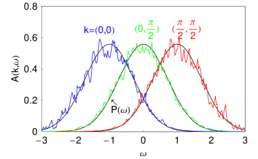
Figure 2: (Color online) ARPES spectral function (II) for $36\times 36$ cluster averaged over 100 random realizations of Coulomb disorder. Concentration of defects is $C=0.6\%$. Values of momenta are ${\bm{k}}=(\pi/2,\pi/2)$, $(0,\pi/2)$, and $(0,0)$. Smooth lines correspond to energy dispersion $\omega=-\epsilon_{\bf k}$ [with $\epsilon_{\bf k}$ given by Eq. (20)], broadened according to Eqs. (15), (16), and (5). In these equations, we set $L=36/\sqrt{\pi}$ and $a_{d}=1$.

Fig. 2 shows the resulting ARPES spectral function at three different momenta ${\bm{k}}=(\pi/2,\pi/2)$, $(0,\pi/2)$, $(0,0)$ together with the analytical distribution (15) of the Coulomb potential $P(\omega)$. In this pedagogical example where the cluster size is certainly smaller than size of experimental samples, we choose $C=0.6\%$. There is an excellent agreement of the line shape and the line width between $P(\omega)$ and $A({\bf k},\omega)$ in all three momenta. This confirms our statement that Eq. (15) describes a Gaussian broadening of ARPES spectra in an insulator due to surface Coulomb defects, and implies that according to Eq. (II), the concentration of $0.6\%$ surface defects (for one charge species) is sufficient to explain the observed broadening in La₂CuO₄, and $0.2\%$ is sufficient for Ca₂CuO₂Cl₂. It is worth mentioning that this broadening is a fairly general mechanism that works not only for Mott insulators, it is also valid for usual band insulators.

How one can check experimentally validity of the suggested broadening mechanism? There are a few “handles” in Eq. (16): the infrared cutoff $L$, the ultraviolet cutoff $a_{d}$, the density $C$ and the potential $V$ of the defects. One can vary $a_{d}$ by probing deeper layers (e.g., using different photon energies): for the top layer $a_{d}=1$, for the second one $a_{d}=4.4$, for the third layer $a_{d}=7.8$, etc. Therefore the width for the second layer must be by 5-6% smaller than the width for the top one, the width for the third layer is further reduced by 2-3%. These are rather small effects. Another possible “handle” is the infrared cutoff $L$. It is natural to assume that $L$ is equal to the radius of the incident photon beam. In this case focusing/defocusing of the beam changes the width accordingly. For instance, the radius variation from $L=1\mu m$ to $L=1mm$ gives rise to a sizable variation of the width by  30%. It can be noticed, however, that the width is most sensitive to the amount and the nature of defects, so systematic studies of the width variation as a function of the surface quality might be useful.

III Spectrum of Copper Nuclear Quadrupole Resonance

In this section we examine the effect of Coulomb disorder on the NQR spectrum. Doping dependence of ⁶³Cu NQR in La_2-xSr_xCuO₄ has been studied in detail in Refs. imai93, and Singer02, , which show that in the undoped parent compound the NQR spectrum is comprised of a very narrow line (centered at frequency $33.05$ MHz at T=600 K). The spectrum is shifted to higher frequency upon hole doping, with a line width roughly proportional to doping. Since NQR is a local probe of real space hole distribution, Haase04 the broad spectrum indicates a very inhomogeneous profile of hole density. Singer02 Another interesting feature is that NQR spectra in doped samples show a double structure: a secondary hump (the ”B-line”) appears at a frequency higher than the broad main line. The origin of the B-line is attributed to the Cu sites that are directly underneath the Sr substitutions. We will show the experimental data and compare it with our results later in this section.

The NQR spectrum is obtained by calculating the hole density distribution which is spatially nonuniform due to disorder. The model used in the previous section is modified here as follows. Since NQR is a bulk sensitive measurement the surface defects are not relevant, and disorder effect is solely due to the Coulomb potential of randomly distributed Sr-dopants. The total number of out-of-plane Sr ions is equal to that of the holes, as suggested by the doping mechanism of La_2-xSr_xCuO₄, and each Sr-defect brings about a negative charge. The concentration of negative defects is therefore equal to doping, and no positive defects are present. Further, the strength of Coulomb interaction is reduced comparing to the surface case, because the bulk dielectric constant is larger: $\epsilon\simeq 2\epsilon_{s}$, see Eq. (2). We denote the effective dimensionless charge in bulk as

$$Q \approx \frac{0.5V}{J}\approx 0.75\;,$$ (25)

which is half of the surface dimensionless charge $Q^{s}$, Eq. (22). The interaction of a hole with Sr ions is then

$$H_{h-Sr} = \sum_{l,i}{\cal U}_{li}c^{{\dagger}}_{i}c_{i}\;,$$

$${\cal U}_{li} = -\frac{Q}{\sqrt{|{\bf R}_{l}-{\bf r}_{i}|^{2}+a_{d}^{2}}}\;.$$ (26)

Similarly, the Coulomb interaction between holes is described by

$$H_{int} = \sum_{ij}U_{ij}c^{{\dagger}}_{i}c_{i}c^{{\dagger}}_{j}c_{j}\ ,$$

$$U_{ij} = \frac{Q}{\sqrt{|{\bf r}_{i}-{\bf r}_{j}|^{2}+a^{2}_{d}}}\;,$$ (27)

where we use the same cutoff $a_{d}=1$ to represent the size of the Zhang-Rice singlet.

We further consider the effect of multilayer screening in bulk of La_2-xSr_xCuO₄ that contains a periodic structure of CuO₂ layers along $c$-axes. The electric field of a charge in a particular layer is substantially screened and deformed by the other layers, as shown schematically in Fig. 3, due to their large polarizability.

Figure 3: Screening of in-plane Coulomb interaction by other layers. Dashed lines shows electric field of an in-plane charge bent due to a large polarizability of “other layers”.

In principle, one needs to perform a self-consistent calculation that includes multiple layers to account for this effect. Unfortunately, such a calculation is too expensive computationally. However, one can consider the following two limiting cases where analytical descriptions are available. The first case is that at extremely small doping, the polarizability of other layers is negligible, hence we recover the single layer formulae in Eqs. (III) and (III). The second case is that at sufficiently large doping, the high polarizability implies that the electric field generated from one layer is practically perpendicular to the surface of its nearest layers as it is shown in Fig. 3. In this case, one can simply apply the method of image to account for the screening due to other layers, by assuming that each layer is placed between two highly polarizable media. The interactions described in Eqs. (III) and (III) are then replaced by Ho09

$${\cal U}_{li} \to -Q\left(\frac{1}{\sqrt{|{\bf R}_{l}-{\bf r}_{i}|^{2}+a_{d}^{2}}}\right.$$

$$\left.+\sum_{n=1}^{\infty}\frac{2(-1)^{n}}{\sqrt{|{\bf R}_{l}-{\bf r}_{i}|^{2}+(2nd)^{2}}}\right)\ ,$$

$$U_{ij} \to Q\left(\frac{1}{\sqrt{|{\bf r}_{i}-{\bf r}_{j}|^{2}+a_{d}^{2}}}\right.$$ (28)

$$\left.+\sum_{n=1}^{\infty}\frac{2(-1)^{n}}{\sqrt{|{\bf r}_{i}-{\bf r}_{j}|^{2}+(2nd)^{2}}}\right)\;,$$

where $d=13.2\AA\to 3.5$ is the separation between layers. The crossover between these two limiting cases corresponds to the situation when the in-plane dielectric constant due to holes is equal to the ionic dielectric constant, which takes place at $x\approx 1\%$.Chen91 Since we are interested in the range of $x\geq 1\%$, relevant to the NQR data discussed below, Eq. (III) is applied to all finite doping cases in our simulations. Accuracy of this approximation is somewhat questionable at $x=1\%$, but it is fairly reasonable at higher dopings.

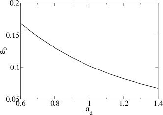
Figure 4: The hole-Sr binding energy as a function of the short-range cutoff $a_{d}$. We recall that we set $J=1$. The interlayer screening is taken into account according to Eq. (III).

Here we give more details about the choice of $a_{d}$, under the condition that the multilayer screening has been accounted for via Eq. (III). The main reason for this short range cutoff is the size of the Zhang-Rice singlet, which a priori yields $a_{d}\approx 1$. On the other hand, the value of $a_{d}$ should properly restore the binding energy of a single hole trapped around a Sr ion, which is known to be $\epsilon_{b}\sim 10\ \mbox{meV}\sim 0.1J$.kotov07 To estimate $\epsilon_{b}$, we assume that there exists a large enough doping range where multilayer screening takes place via Eq. (III), while the doping is still small enough that the in-plane hole-hole interaction can be ignored, and diagonalize the Hamiltonian $H=H_{t}+H_{h-Sr}$ with only one Sr present. The resulting binding energy versus $a_{d}$ is shown in Fig. 4, where we found that $a_{d}=1$ indeed gives the correct binding energy. For extremely low doping $x\ll 1\%$, we adopt the unscreened potential Eq. (III) without considering other layers, and found that $a_{d}=1$ gives $\epsilon_{b}\approx 0.23J\approx 30$ meV. This demonstrates the importance of the multilayer screening at doping $x\geq 1\%$. The value $a_{d}=1$ is adopted throughout this work.

The full Hamiltonian

$$H=H_{t}+H_{h-Sr}+H_{int}$$ (29)

can be diagonalized by the following analysis. The dimensionless parameter that characterizes the strength of interaction in a 2D Coulomb gas isAshcroft

$$r_{s}=\frac{m^{*}e^{2}}{\epsilon\hbar^{2}\sqrt{\pi n}}\approx\frac{0.36}{\sqrt{\pi x}}\ .$$ (30)

We see that even at $x=2\%$ the value of $r_{s}$ is still small $r_{s}\approx 1.4$. Moreover, the multilayer screening introduced in Eq. (III) further reduces this value to $r_{s}\to 1$. Therefore, we are safely in the weak coupling regime where the Hartree-Fock treatment is adequate. Notice that the hole dynamics are certainly strongly correlated at the length scale about a few lattice spacing. These are Hubbard or t-J model correlations which result in the dispersion of dressed holes, Eq. (20). Here the term ”weak coupling” refers to the long range Coulomb interaction between holes at the length scale $\geq 1/\sqrt{x}$, where the effect of the short-range strong correlations is already taken care of by adopting the dispersion (20). The Hartree-Fock decomposition is then applied to the hole-hole interaction

$$H_{int}\to\sum_{ij}U_{ij}\langle c^{{\dagger}}_{i}c_{i}\rangle c^{{\dagger}}_{j}c_{j}-\sum_{ij}U_{ij}\langle c^{{\dagger}}_{i}c_{j}\rangle c^{{\dagger}}_{j}c_{i}\;.$$ (31)

The diagonalization is again done in a $36\times 36$ cluster with periodic boundary conditions (torus). Expectation values $\langle c^{{\dagger}}_{i}c_{i}\rangle$ and $\langle c^{{\dagger}}_{i}c_{j}\rangle$ can be calculated by

$$\langle c^{{\dagger}}_{i}c_{i}\rangle = \sum_{n}|\alpha_{n}(i)|^{2}f(E_{n})\ ,$$

$$\langle c^{{\dagger}}_{i}c_{j}\rangle = \sum_{n}\alpha_{n}(i)^{*}\alpha_{n}(j)f(E_{n})\ ,$$ (32)

where

$$f(E_{n})=\frac{1}{e^{(E_{n}-\mu)/T}-1}$$ (33)

is the Fermi-Dirac distribution.

To determine the macroscopic chemical potential in our simulation, we adopt the following procedure. The chemical potential at either zero or finite temperature in each defect configuration is determined via the charge neutrality condition, i.e. the number of negative defects is equal to the number of holes. The average value of the chemical potential, denoted by $\mu$, is then calculated out of 100 defect configurations taken. We then shift the entire energy spectrum of each particular configuration in such a way that the chemical potential of the configuration is equal to this mean value $\mu$, which is the macroscopic chemical potential.

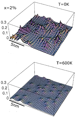
Figure 5: (Color online) Plots of the hole density in a CuO₂ layer deep in the bulk, for a particular realization of random Sr positions, at doping $x=0.02$ and two different temperatures $T=0$ and 600 K. The length scale 5 nm ($\approx 13a_{0}$) is shown.

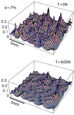
Figure 6: (Color online) Plots of the hole density in a CuO₂ layer deep in the bulk, for a particular realization of random Sr positions, at doping $x=0.07$ and two different temperatures $T=0$ and 600 K.

Hole density plots $n_{i}=\langle c^{{\dagger}}_{i}c_{i}\rangle$ for particular realizations at $x=0.02$ and $x=0.07$ are shown in Figs. 5 and 6, respectively, for two different temperatures $T=0$ and $T=600$ K. One sees very inhomogeneous density profiles, with a characteristic length scale of the order of a few nanometers. Similar nanoscale charge inhomogeneities, that closely resemble the STM images of underdoped cuprates (see, e.g., Refs. Koh07, , Koh04, ), have been also reported in previous studies Wan01 ; Wan02 ; Zho07 . Interestingly, we find that increasing temperature substantially reduces the inhomogeneity (compare upper and lower panels in Figs. 5 and 6). This has consequences for NQR spectra which we address in the following.

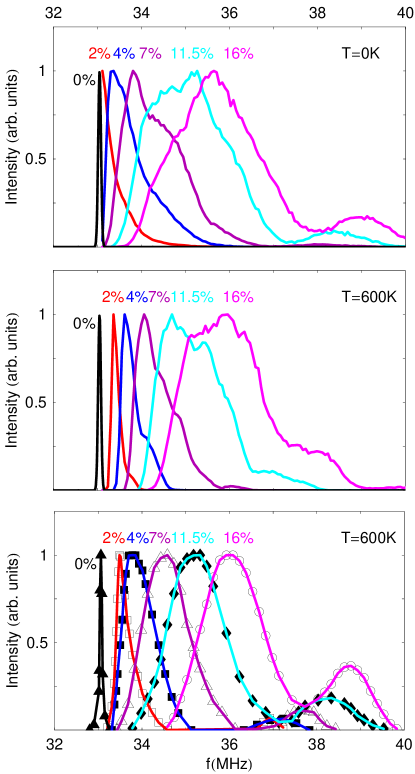
Figure 7: (Color online) The calculated (upper and middle panels) and experimental Singer02 (lower panel) ⁶³Cu NQR spectra in La_2-xSr_xCuO₄ at different doping levels $x$= 0.02, 0.04, 0.07, 0.115, and 0.16. The narrow line at $f=33.05MHz$ imai93 corresponds to the parent compound, $x=0$. Apart from broadening of the spectra, doping results also in a high-frequency structure similar to the “B-line” observed in the experiment Singer02 . Note that linewidth at T=600 K is smaller than that at zero temperature.

The NQR frequency at a particular site $i$ is related to the hole density $n_{i}$ byHaase04

$$\nu_{i}\approx(33.05+19\cdot n_{i})MHz\ .$$ (34)

Thus, the entire NQR spectrum, which effectively sums over all sites in the sample, is proportional to the probability distribution of the hole density ${\cal P}(n)$, up to a constant shift 33.05 MHz corresponding to the parent compound imai93 . Calculated NQR spectra for $T=0$ and $T=600$ K are presented in the upper and in the middle panels of Fig. 7, respectively. The experimental plots of Refs. Singer02, and imai93, for La_2-xSr_xCuO₄ at different dopings and T=600 K are shown in the lower panel for comparison. One sees that the shift and the broadening of the spectrum upon doping are well reproduced by the theory, with the linewidth consistent with experimental data. Surprisingly, the agreement is reasonable even at 16% doping which is certainly too large for our low doping theory. The mechanism that narrows the linewidth with temperature Singer02 is also understood: increasing temperature reduces the spatial inhomogeneity of density profile, as shown in Figs. 5 and 6, which results in a narrower probability distribution ${\cal P}(n)$, and hence the narrower NQR spectrum (compare the upper and the middle panels in Fig. 7). Although our simple model does not take into account the direct action of the Sr ion Coulomb field on the nearest Cu nuclei, which is believed to be the main origin of the high frequency ”B-line”,Singer02 in our numerics we do see a shoulder-like structure emerging at high frequency. A detailed investigation shows that this structure is associated with holes that are trapped around local potential minimum due to occasionally clustered $2$ to $3$ Sr defects. We suspect that these trapped holes, albeit not the main reason for the ”B-structure”, can have a certain contribution to it. The most important point here is that the main line is well understood in our model, which properly captures the hole density distribution and the screening effects in presence of Sr defects.

IV Density of states and Anderson localization in $\mbox{CuO}_{2}$ layer in the bulk

In this section we address the issue of the bulk DOS in presence of disorder, and relation of the DOS to the normal state dc electrical conductivity. It is known that La_2-xSr_xCuO₄ exhibits the variable range hopping conductance at small doping $x<0.055$;Kastner98 ; ando02 . This indicates a strong localization of holes by Sr Coulomb potential. It has been suggested that the onset of superconductivity at $x>0.055$ is due to percolation of the bound states. sushkov05 The hole density plots shown in Figs. 5 and 6 support this suggestion: the hole density at $x=0.02$ $(T=0)$ vanishes in large areas of the system, signaturing a highly localized density profile, while the density at $x=0.07$ $(T=0)$ is nonzero practically everywhere in the system, so wave functions are highly overlapped.

To study the problem in more detail, we have calculated the 2D density of states, $\rho(\epsilon)$, via the standard definition:

$$\rho(\epsilon)=\frac{1}{N}\sum_{n}\delta(\epsilon-E_{n})\;.$$ (35)

Fig. 8 shows the DOS calculated using the eigenenergies of Eq. (29) and fixing the chemical potential as described in the previous section. One sees clearly a full reduction of DOS at the chemical potential as expected by the Coulomb gap theory in 2D systems SE . The size of the gap is about $\Delta_{C}\sim 2.0-2.5$ meV at $x=0.02$ and it decreases to about $1.5-2.0$ meV at $x=0.07$. We define $\Delta_{C}$ such that the total width of the gap structure in DOS is $2\Delta_{C}$ as indicated in the lower panel of Fig. 10. Importantly, the gap smoothly evolves through the percolation point $x=0.055$. This implies that for single particle dynamics the system remains an Anderson insulator even after percolation. Probably at even larger doping, $x>0.1$, the Coulomb gap smoothly evolves to the logarithmic reduction of DOS corresponding to the weak localization theory.AAP Unfortunately, we are not able to trace this crossover because the relatively small size of the cluster, 36$\times$36, limits our accuracy of the gap calculation at the level $\sim 1$ meV. The insulating behavior across the percolation point $x=0.055$ obtained in the present calculation agrees perfectly with the experimental data Ando95 ; Boebinger96 where the in-plane resistivity, measured in a very strong magnetic field that destroys superconductivity, shows an insulating behaviour below $\sim 50$ K for a wide doping range up to $x\approx 15\%$.

The DOS displayed in Fig. 8 exhibits oscillations above chemical potential. These oscillations is a byproduct of the finite size of the cluster. Maxima of the DOS correspond to degenerate states with dispersion (20) on the $36\times 36$ torus. The oscillations must certainly disappear in the thermodynamics limit. However, oscillations of this kind also have an interesting physical meaning. In particular, the $x=0.02$ plot in Fig. 8 indicates that while the quantum states near the chemical potential are strongly localized, the high-energy states well above the chemical potential are quite extended with a mean free path exceeding the size of the cluster used. Similarly, the smeared oscillations in Fig. 8, $x=0.07$ indicate that the mean free path is comparable with or less than the cluster size.

Figure 8: The hole DOS in $\mbox{CuO}_{2}$ layer deep in the bulk at dopings $x=0.02$ and $x=0.07$. DOS vanishes at the chemical potential indicating the Coulomb gap which gradually decreases with doping.

V Evolution of ARPES spectra with doping, and Density of States in the Surface $\mbox{CuO}_{2}$ layer

To study the evolution of ARPES spectrum upon doping, we apply the above Hartree-Fock treatment and interlayer screening picture to the top CuO₂ plane near the surface. The ARPES linewidth is determined now by a combined action of two types of disorder: the surface defects, as described by $H_{h-d}$ in Sec. II, and a randomly distributed Sr-dopant ions described by $H_{h-Sr}$ in Sec. III. To be specific, we fix here the concentration of positively/negatively charged surface defects to be $C_{+}=C_{-}=C=0.6\%$, as required to fit the ARPES linewidth in La₂CuO₄, see Eq. (II). We assume that concentration $C$ is independent on Sr-doping since it is determined by the surface properties unrelated to doping. Total concentration for negatively charged defects is then $x+C=x+0.6\%$, counting both Sr-dopants and the negatively charged surface defects. Dimensionless charge $Q^{s}$ is again described by Eq. (22), which is twice of its bulk value $Q$ due to the reduced dielectric constant (2) on the surface. Consequently, this enhances the disorder effects on the surface as we will see below. The multilayer screening of the interactions on a cleaved surface is also different from that in the bulk, Eq. (III), because even though other planes are still considered as highly polarizable, and hence the method of image is still valid for $x\geq 1\%$, the cleaved surface is now considered as located at a distance $d$ above a polarizable media, see Fig. 9, instead of being sandwiched between two polarizable slabs. Collecting all these effects, we have

$$H_{h-d}+H_{h-Sr} = \sum_{l,i}{\cal U}_{li}c^{{\dagger}}_{i}c_{i}\;,$$ (36)

where a disorder potential, originating either from surface or Sr defects located at position ${\bf R}_{l}$, is given by

$${\cal U}_{li} \to \pm Q^{s}\left(\frac{1}{\sqrt{|{\bf R}_{l}-{\bf r}_{i}|^{2}+a_{d}^{2}}}\right.$$ (37)

$$\left.\;\;\;\;+\frac{-1}{\sqrt{|{\bf R}_{l}-{\bf r}_{i}|^{2}+(2d)^{2}}}\right)\;.$$

The difference between $H_{h-d}$ and $H_{h-Sr}$ is only in the sign of $Q^{s}$: $H_{h-Sr}$ potential is always attractive and has charge $-Q^{s}$, while its sign in $H_{h-d}$ depends on charge of the surface defect which can be either positive or negative. Similarly, the hole-hole interaction reads as

$$H_{int} = \sum_{ij}U_{ij}c^{{\dagger}}_{i}c_{i}c^{{\dagger}}_{j}c_{j}\;,$$ (38)

$$U_{ij} \to Q^{s}\left(\frac{1}{\sqrt{|{\bf r}_{i}-{\bf r}_{j}|^{2}+a_{d}^{2}}}+\frac{-1}{\sqrt{|{\bf r}_{i}-{\bf r}_{j}|^{2}+(2d)^{2}}}\right).$$

We then diagonalize the full Hamiltonian

$$H=H_{t}+H_{h-d}+H_{h-Sr}+H_{int}$$ (39)

following the Hartree-Fock treatment described in Eqs. (31) to (33). The procedure described in Sec. III is again applied to determine the macroscopic chemical potential.

Figure 9: Screening of in-plane Coulomb interaction in the top layer by other layers underneath. Dashed lines shows electric field of an in-plane charge bent due to polarization of “other layers”.

First, we discuss DOS obtained from the numerical diagonalization. Fig. 10 shows the calculated DOS for the top CuO₂ layer, where one clearly sees a Coulomb gap of the order of $\Delta_{C}\sim 0.1J\sim 10$ meV opening at the chemical potential. Comparing the result with the bulk DOS shown in Fig. 8, we see a significant difference which is due to enhanced dimensionless charge $Q^{s}$: a 2D Coulomb gap scales approximately as $Q^{2}$, see Ref. SE, .

There are no sizable oscillations of the DOS in Fig. 10. This means that the hole mean free path even well above the chemical potential is much smaller than the cluster size.

Notice that values of the chemical potential on the surface, Fig. 10, are somewhat different from those in the bulk, Fig. 8. This difference is a byproduct of our approximations. A tiny surface charging energy and/or a tiny surface lattice deformation due to La $\to$ Sr substitutions can tune up the surface chemical potential from its bulk value. Due to these effects, which are not taken into account in the present model, we cannot compare the calculated chemical potential with experimental values. Although these effects can shift the chemical potential and overall energy scales, they do not influence the wave functions and the shape of DOS.

Figure 10: The hole DOS in the surface $\mbox{CuO}_{2}$ layer at dopings $x=0.02$ and $x=0.07$. DOS vanishes at the chemical potential indicating the Coulomb gap $\Delta_{C}$. The size of the gap, $\Delta_{C}\sim 10$ meV, is larger than that in the bulk (see Fig. 8).

Now, we turn to the ARPES spectra at finite dopings. The spectral functions are again calculated by using the eigenstates and eigenenergies given by exact diagonalization. Notice that at finite doping and zero temperature only states above chemical potential are considered. This is because we are working in the hole representation, while ARPES spectrum is associated with the electron spectral function, therefore only states occupied by electrons $E_{n}>\mu$ should be summed over in Eq. (II). It is also convenient to shift origin of the momentum to the dispersion minimum $(\pi/2,\pi/2)$,

$${\bf k}=(\pi/2,\pi/2)+{\bf p}\;,$$ (40)

and present the spectral function in terms of ${\bf p}$. In our model $A({\bf p},\omega)$ is roughly symmetric around the dispersion minimum, $A({\bf p},\omega)\approx A(|{\bf p}|,\omega)$. In addition, because of the $36\times 36$ finite cluster size, we can only calculate certain discrete values of momentum, ${\bf p}=\frac{\pi}{18}(m,n)$, where m,n are integers. On the other hand, the doping level $x$ can be varied continuously. In Fig. 11, we present spectral functions calculated for the following momenta in the nodal direction

$${\bf p}_{0} = 0\ ,$$

$${\bf p}_{1} = \left(\frac{\pi}{18},\frac{\pi}{18}\right)\ ,$$

$${\bf p}_{2} = \left(\frac{2\pi}{18},\frac{2\pi}{18}\right)\ ,$$

$${\bf p}_{3} = \left(\frac{3\pi}{18},\frac{3\pi}{18}\right)\ ,$$ (41)

and for $x=0.01\ -\ 0.11$. Surprisingly, we see very narrow lines with the width of the order $\Gamma\sim 0.2J\sim 30$ meV, in spite of the very strong disorder. This is certainly due to the Coulomb screening of both the surface defects and Sr dopant potentials. This residual “small” width $\Gamma\sim 30$ meV is due to the hole scattering from the residual (locally unscreened) part of the random potential. Remarkably, the residual width is quite universal, it is practically independent of doping. On a qualitative level, this (somewhat unexpected) observation can be understood as a result of two opposite trends: On the one hand, more Sr-doping increases amount of disorder but, at the same time, adding more holes reduces an effective scattering amplitude on each Sr-defect because of better screening. Within the present low energy effective theory, which is valid up to energies $E\sim J\sim 100-200$meV, the residual width is also energy/momentum independent.

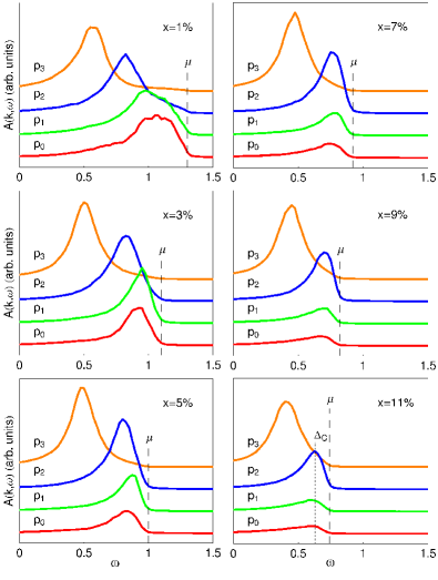
Figure 11: (Color online) The electron spectral function $A({\bf k},\omega)$ at doping levels $x=0.01,0.03,0.05,0.07,0.09,0.11$ calculated for momenta ${\bf p}_{0}$, ${\bf p}_{1}$, ${\bf p}_{2}$, ${\bf p}_{3}$ specified in Eq. (V). The Coulomb gap $\Delta_{C}$ is highlighted in the $x=0.11$ plot.

Finally, the evolution of the small Fermi surface upon doping can be considered. We first notice that in the homogeneous case the dispersion is given by Eq. (20). Hence the Fermi momentum $p_{F}$ and the doping $x$ are related as

$$x=\frac{p_{F}^{2}}{\pi}\;,$$ (42)

if doping is small and the dispersion is roughly parabolic. Therefore, $p_{F}=p_{1}$ at $x\approx 0.02$ and $p_{F}=p_{2}$ at $x\approx 0.08$. Interestingly, the relation (42) remains qualitatively correct even in the presence of strong disorder. This can be seen by the following analysis that extracts the Fermi momentum: We know that without disorder, the ARPES intensity at $p$ below $p_{F}$ vanishes at any finite doping, since the momentum is inside hole Fermi surface and no electron with this momentum can be excited. Therefore, the ARPES intensities at this momentum (red curves) in Fig. 11 are nonzero only because of disorder. The intensity decays very quickly when doping is increasing. We found that maxima of spectral functions are never exactly at the chemical potential, as one would expect in a system without disorder. Instead, we see that the maximum of each line gets closer to the chemical potential as doping is increased, but stops at an energy scale $\Delta_{C}\sim 0.1J\sim 10$ meV below the chemical potential. This is clearly due to the Coulomb gap opening in the DOS, as shown in Fig. 10, which suppresses the spectral function within $\mu-\Delta_{C}<\epsilon<\mu$ and shifts the maximum. The maximum of the $p=p_{1}$ line (green curves) approaches its rightmost position $\mu-\Delta_{C}$ at $x\approx 0.03$, so at this doping we say the ”Fermi surface” crosses the momentum $p=p_{1}$. Similarly, the maximum of the $p=p_{2}$ line (blue curves) approaches its rightmost position at $x\approx 0.09$, hence the Fermi surface crosses $p=p_{2}$ at this doping. Following this procedure, we can identify the ”Fermi momentum” at each doping, which can be compared with the experiments, although only discrete values at ${\bf p}=\frac{\pi}{18}(m,n)$ can be identified.

It should be stressed that our aim here is to study the Coulomb disorder and its influence on the quasiparticle peak. Strong (Hubbard or t-J model) correlations are taken into account only via effective dispersion (20) of the holon. In all other respects we disregard the spin degrees of freedom. Therefore, we do not reproduce the asymmetry of the ARPES spectral function $A({\bf p},\omega)$ with respect to the boundary of the magnetic Brillouin zone, and also strongly underestimate the ARPES intensity below the quasiparticle peaks, seen in the experiment as a pronounced ”hump” structure. In spite of these drawbacks, the theory allows us to address the issue of evolution of the quasiparticle peak with disorder/doping. In particular, our theory explains why the ARPES lines in doped cuprates are relatively narrow in spite of the very strong Coulomb disorder. Ino2000 ; Yoshida03 ; Yoshida07 ; Shen04 ; Shen07

Another interesting result obtained in this section is the predicted Coulomb gap $\sim 10$ meV in density of states that could be observed by surface sensitive probes like the STM and ARPES. In fact, the gap features of this scale are present in the STM data for underdoped cuprates (see, e.g., Ref. Koh04, ), and are typically attributed to the (local) pairing gap; the Coulomb gap might be an additional origin of these low-energy structures.

VI Conclusions

In this paper, a comprehensive study of Coulomb disorder effects in undoped and lightly-doped cuprates is performed, and the main results can be summarized as follows.

1. We have demonstrated that a very small amount of surface Coulomb defects leads to a dramatic broadening of ARPES spectrum in insulators. In particular, a concentration of defects about just a fraction of 1% is sufficient to explain observed ARPES line widths in La₂CuO₄ and Ca₂CuO₂Cl₂. The broadened spectrum displays a Gaussian shape, consistent with experiments. Shen04 In the end of section II we have discussed possible ways to check the suggested broadening mechanism experimentally.

2. Doping process, e.g., random substitutions La $\to$ Sr in La_2-xSr_xCuO₄, intrinsically creates strong inhomogeneity in the system. By performing Hartree-Fock calculations, we show that due to the strong Coulomb screening, ARPES lines obtain a very narrow width ($\Gamma\sim 30-40$ meV) as soon as doping is higher than $\sim 1\%$, in spite of the very strong disorder. These results provide a natural explanation for why the ARPES spectra undergo radical changes – from very broad Gaussian to narrow quasiparticle peaks – upon just a few percent doping of parent compounds. The residual “small” width $\Gamma\approx 30-40$ meV is due to the hole scattering from the residual (locally unscreened) part of the random potential. The residual width is quite universal, it is practically independent of doping/energy/momentum.

3. The calculation of the surface density of states demonstrates that the top CuO₂ layer of La_2-xSr_xCuO₄ is always in the Anderson localization regime, and we predict the Coulomb gap of the order of $\sim 10$ meV which could be observed with STM and/or ARPES experiments.

4. The calculation of the bulk density of states also shows the Coulomb gap of the order of a few meV. The gap evolves smoothly through the percolation point $x=0.055$. Hence the system remains in the Anderson localization regime, and this explains the insulating behavior observed in transport properties at high magnetic fields. Ando95 ; Boebinger96

5. Considering Sr-doping induced disorder in La_2-xSr_xCuO₄, we find a very inhomogeneous hole density profile which yields a broad NQR spectrum. The calculated doping and temperature dependencies of NQR lineshapes are consistent with experiments.

Altogether, the results reported here highlight a significant role played by Coulomb disorder effects in cuprates. In particular, screening of Coulomb defects (either of extrinsic origin or introduced by dopant ions) results in a dramatic evolution of physical properties upon doping. In this work, we focused mostly on the charge degrees of freedom, accounting for underlying magnetic correlations merely via a properly renormalized dispersion of the mobile holes. It remains a challenge to incorporate the magnetic degrees of freedom into the model explicitly, exploring thereby the coupled charge and spin dynamics in cuprates at short length scales.

VII acknowledgments

Useful discussions with L.P. Ho, A. Fabricio Albuquerque, C.J. Hamer, J. Oitmaa, and T. Valla are acknowledged. We would like to thank P.M. Singer and T. Imai for sharing and discussion of their NQR data. G.Kh. thanks the School of Physics and Gordon Godfrey fund, UNSW, for kind hospitality. O.P.S. thanks the MPI Stuttgart for kind hospitality. Numerical calculation is done by the facilities of University of Florida High Performance Cluster.

References

- (1) A. Damascelli, Z. Hussain, and Z.-X. Shen, Rev. Mod. Phys. 75, 473 (2003).
- (2) B.O. Wells, Z.-X. Shen, A. Matsuura, D.M. King, M.A. Kastner, M. Greven, and R.J. Birgeneau, Phys. Rev. Lett. 74, 964 (1995).
- (3) J.J.M. Pothuizen, R. Eder, N.T. Hien, M. Matoba, A.A. Menovsky, and G.A. Sawatzky, Phys. Rev. Lett. 78, 717 (1997).
- (4) T. Tohyama and S. Maekawa, Supercond. Sci. Technol. 13, R17 (2000).
- (5) O.P. Sushkov, G.A. Sawatzky, R. Eder, and H. Eskes, Phys. Rev. B 56, 11769 (1997).
- (6) A. Ino, C. Kim, M. Nakamura, T. Yoshida, T. Mizokawa, Z.-X. Shen, A. Fujimori, T. Kakeshita, H. Eisaki, and S. Uchida, Phys. Rev. B 62, 4137 (2000).
- (7) T. Yoshida, X.J. Zhou, T. Sasagawa, W.L. Yang, P.V. Bogdanov, A. Lanzara, Z. Hussain, T. Mizokawa, A. Fujimori, H. Eisaki, Z.-X. Shen, T. Kakeshita, and S. Uchida, Phys. Rev. Lett. 91, 027001 (2003).
- (8) T. Yoshida, X.J. Zhou, D.H. Lu, S. Komiya, Y. Ando, H. Eisaki, T. Kakeshita, S. Uchida, Z. Hussain, Z.-X. Shen, and A. Fujimori, J. Phys. Condens. Matter 19, 125209 (2007).
- (9) K.M. Shen, F. Ronning, D.H. Lu, W.S. Lee, N.J.C. Ingle, W. Meevasana, F. Baumberger, A. Damascelli, N.P. Armitage, L.L. Miller, Y. Kohsaka, M. Azuma, M. Takano, H. Takagi, and Z.-X. Shen, Phys. Rev. Lett. 93, 267002 (2004).
- (10) K.M. Shen, F. Ronning, W. Meevasana, D.H. Lu, N.J.C. Ingle, F. Baumberger, W.S. Lee, L.L. Miller, Y. Kohsaka, M. Azuma, M. Takano, H. Takagi, and Z.-X. Shen, Phys. Rev. B 75, 075115 (2007).
- (11) T. Imai, C.P. Slichter, K. Yoshimura, and K. Kosuge, Phys. Rev. Lett. 70, 1002 (1993).
- (12) P.M. Singer, A.W. Hunt, and T. Imai, Phys. Rev. Lett. 88, 047602 (2002).
- (13) A.S. Mishchenko and N. Nagaosa, Phys. Rev. Lett. 93, 036402 (2004).
- (14) O. Gunnarsson and O. Rosch, J. Phys.: Condens. Matter 20, 043201 (2008).
- (15) P. Prelovsek, R. Zeyher, and P. Horsch, Phys. Rev. Lett. 96, 086402 (2006).
- (16) C.Y. Chen, R.J. Birgeneau, M.A. Kastner, N.W. Preyer, and T. Thio, Phys. Rev. B 43, 392 (1991).
- (17) M.A. Kastner, R.J. Birgeneau, G. Shirane, and Y. Endoh, Rev. Mod. Phys. 70, 897 (1998).
- (18) G. De Filippis, V. Cataudella, A.S. Mishchenko and N. Nagaosa, Phys. Rev. Lett. 99, 146405 (2007).
- (19) Y. Kohsaka, C. Taylor, K. Fujita, A. Schmidt, C. Lupien, T. Hanaguri, M. Azuma, M. Takano, H. Eisaki, H. Takagi, S. Uchida, and J.C. Davis, Science 315, 1380 (2007).
- (20) T. Hanaguri, C. Lupien, Y. Kohsaka, D.-H. Lee, M. Azuma, M. Takano, H. Takagi, and J.C. Davis, Nature 430, 1001 (2004).
- (21) B.I. Shklovskii and A.L. Efros, Electronic properties of doped semiconductors (Springer-Verlag, Berlin, New York, 1984).
- (22) B.L. Altshuler, A.G. Aronov, and P.A. Lee, Phys. Rev. Lett. 44, 1288 (1980).
- (23) Y. Ando, K. Segawa, S. Komiya, and A.N. Lavrov, Phys. Rev. Lett. 88, 137005 (2002).
- (24) Y. Ando, G.S. Boebinger, A. Passner, T. Kimura, and K. Kishio, Phys. Rev. Lett. 75, 4662 (1995).
- (25) G.S. Boebinger, Y. Ando, A. Passner, T. Kimura, M. Okuya, J. Shimoyama, K. Kishio, K. Tamasaku, N. Ichikawa, and S. Uchida, Phys. Rev. Lett. 77, 5417 (1996).
- (26) V.V. Batygin, I.N. Toptygin, Problems in electrodynamics (Academic Press, London, New York, 1978).
- (27) J. Haase, O.P. Sushkov, P. Horsch, and G.V.M. Williams, Phys. Rev. B 69, 094504 (2004).
- (28) L.H. Ho, A.P. Micolich, A.R. Hamilton, and O.P. Sushkov, arXiv:0904.3786.
- (29) V.N. Kotov, O.P. Sushkov, M.B. Silva Neto, L. Benfatto, and A.H. Castro Neto, Phys. Rev. B 76, 224512 (2007).
- (30) N.W. Ashcroft, N.D. Mermin, Solid state physics (Holt, Rinehart and Winston, New York, 1976).
- (31) Y. Kohsaka, K. Iwaya, S. Satow, T. Hanaguri, M. Azuma, M. Takano, and H. Takagi, Phys. Rev. Lett. 93, 097004 (2004).
- (32) Q.-H. Wang, J. H. Han, and D.-H. Lee, Phys. Rev. B 65, 054501 (2001).
- (33) Z. Wang, J. R. Engelbrecht, S. Wang, and H. Ding, and S.H. Pan, Phys. Rev. B 65, 064509 (2002).
- (34) S. Zhou, H. Ding, and Z. Wang, Phys. Rev. Lett. 98, 076401 (2007).
- (35) O.P. Sushkov and V.N. Kotov, Phys. Rev. Lett. 94, 097005 (2005).