SPINODAL INSTABILITIES IN NUCLEAR MATTER IN A STOCHASTIC RELATIVISTIC MEAN-FIELD APPROACH

Abstract

Spinodal instabilities and early growth of baryon density fluctuations in symmetric nuclear matter are investigated in the basis of stochastic extension of relativistic mean-field approach in the semi-classical approximation. Calculations are compared with the results of non-relativistic calculations based on Skyrme-type effective interactions under similar conditions. A qualitative difference appears in the unstable response of the system: the system exhibits most unstable behavior at higher baryon densities around $\rho_{b}=0.4~{}\rho_{0}$ in the relativistic approach while most unstable behavior occurs at lower baryon densities around $\rho_{b}=0.2~{}\rho_{0}$ in the non-relativistic calculations

I Introduction

Spinodal instability provides a possible dynamical mechanism for fragmentation of a hot piece of nuclear matter produced in heavy-ion collisions. Small amplitude density fluctuations grow rapidly and lead to break-up of the system into an ensemble of clusters R1 . In coming years, experimental investigations of multi-fragmentation reactions in neutron rich nuclear system will provide further understanding of isospin dependence of nuclear matter equation of state at low densities. In theoretical side, extensive investigations of spinodal instabilities have been carried out in the basis of stochastic transport models R2 ; R3 ; R4 ; R5 ; R6 . In particular, the recently proposed stochastic mean-field approach provides a useful tool for a description of dynamics of density fluctuations in the spinodal region R7 . It has been demonstrated that the stochastic mean-field approach incorporates the one-body dissipation and the associated fluctuation mechanism in accordance with the quantal-dissipation fluctuation relation. The approach gives rise to the same result for dispersion of one-body observables that was obtained in a variational approach in a previous work R8 . Furthermore, in recent studies R9 ; R10 by projecting onto macroscopic variables, we deduce transport coefficients for energy dissipation and nucleon exchange in low-energy heavy-ion collisions, which have the similar form with those familiar from the phenomenological nucleon exchange model R11 . These investigations provide a strong support for the fact that the stochastic mean-field approach is a powerful tool for describing low energy nuclear collisions and spinodal dynamics.

In a recent work, we studied the early development of spinodal dynamics of nuclear matter in the basis of the stochastic mean-field approach by employing density-dependent Skyrme-type effective interactions R12 . In the present work, we carry out a similar investigation of early development of density fluctuations in spinodal region of nuclear matter by employing the stochastic extension of the relativistic mean-field theory R13 ; R14 . It has been shown in recent years that the nuclear many-body system is in principal a relativistic system driven by dynamics of large relativistic attractive scalar and repulsive vector fields. Both fields are not much smaller than the nucleon mass and therefore the average nuclear field should be described by Dirac equation. For large components of Dirac spinors, two fields nearly cancel each other leading to relatively small attractive mean field. The small components add up leading to a very large spin orbit term, which is known since early days of nuclear physics. Relativistic models have been used with great success to describe nuclear structure. In recent years, the approach has also been applied for description of nuclear dynamics extended in the framework of time-dependent covariant density functional theory R15 ; R16 . A number of investigations have been carried out on spinodal instabilities in nuclear matter employing relativistic mean-field approaches R17 ; R18 ; R19 . In this work, we consider the stochastic extension of the relativistic mean-field theory in the semi-classical approximation. As illustrated in the non-relativistic limit, stochastic extension of the mean-field theory provides a powerful approach for investigating dynamics of density fluctuations. Employing the stochastic extension of the relativistic mean-field approach, we investigate not only spinodal instabilities but also the early development of density fluctuations in symmetric nuclear matter.

In Section 2, we briefly describe the stochastic extension of the relativistic mean-field theory in the semi-classical approximation. In Section 3, we calculate early growth of baryon density fluctuations, growth rates and phase diagram of dominant modes in symmetric nuclear matter. Conclusions are given in Section 4.

II STOCHASTIC RELATIVISTIC MEAN-FIELD THEORY

The stochastic mean-field approach is based on a very appealing stochastic model proposed for describing deep-inelastic heavy-ion collisions and sub-barrier fusion R20 ; R21 ; R22 . In that model, dynamics of relative motion is coupled to collective surface modes of colliding ions and treated in a classical framework. The initial quantum zero point and thermal fluctuations are incorporated into the calculations in a stochastic manner by generating an ensemble of events according to the initial distribution of collective modes. In the mean-field evolution, coupling of relative motion with all other collective and non-collective modes are automatically taken into account. In the stochastic extension of the mean-field approach, the zero point and thermal fluctuations of the initial state are taken into account in a stochastic manner, in a similar manner presented in refs. R20 ; R21 ; R22 . The initial fluctuations, which are specified by a specific Gaussian random ensemble, are simulated by considering evolution of an ensemble of single-particle density matrices. It is possible to incorporate quantal and thermal fluctuations of the initial state into the relativistic mean-field description in a similar manner.

In refs. R23 ; R24 , the authors derived a relativistic Vlasov equation from the Walecka model in the local density and the semi-classical approximation. In the Walecka model, interaction between nucleons are mediated by a scalar meson with mass $m_{s}$ and a vector meson with mass $m_{\textrm{v}}$, with respective fields denoted as $\phi$ and $V_{\mu}$. Introducing phase space distribution function $f(\vec{r},\vec{p},t)$ for the nucleons, following relativistic Vlasov equation has been obtained ,

$$\frac{\partial}{\partial t}f(\vec{r},\vec{p},t)+\vec{\textrm{v}}\cdot\vec{\nabla}_{r}f(\vec{r},\vec{p},t)-\vec{\nabla}_{r}h(\vec{r},\vec{p})\cdot\vec{\nabla}_{p}f(\vec{r},\vec{p},t)=0.$$ (1)

where $\vec{\textrm{v}}=\vec{p}^{*}/e^{*}$ and $h=e^{*}+g_{\textrm{v}}V_{0}$. The coupling constants of the mesons and the nucleon are denoted by $g_{s}$ and $g_{\textrm{v}}$, for the scalar and the vector mesons, respectively. In these expressions, $\vec{p}^{*}=\vec{p}-g_{\textrm{v}}\vec{V}$ and $e^{*}=(\vec{p}^{*2}+M^{*2})^{1/2}$ with $M^{*}=M-g_{\textrm{s}}\phi$. The nucleon mass is denoted by $M$. In the mean-field approximation, the meson fields are treated as classical fields and their evolutions are determined by the field equations,

$$\left[\frac{\partial^{2}}{\partial{t}^{2}}-\nabla^{2}+m_{\textrm{s}}^{2}\right]\phi(\vec{r},t)=g_{\textrm{s}}\rho_{\textrm{s}}(\vec{r},t)$$ (2)

and

$$\left[\frac{\partial^{2}}{\partial{t}^{2}}-\nabla^{2}+m_{\textrm{v}}^{2}\right]V_{\textrm{v}}(\vec{r},t)=g_{\textrm{v}}\rho_{\textrm{v}}(\vec{r},t).$$ (3)

In these expressions, the baryon density $\rho_{0}(\vec{r},t)=\rho_{\textrm{b}}(\vec{r},t)$, the scalar density $\rho_{\textrm{s}}(\vec{r},t)$, and the current density $\vec{\rho}_{\textrm{v}}(\vec{r},t)$ can be expressed in terms of phase-space distribution function as follows,

$$\rho_{\textrm{b}}(\vec{r},t)=\gamma\int\frac{d^{3}p}{(2\pi)^{3}}f(\vec{r},\vec{p},t),$$ (4)

$$\rho_{\textrm{s}}(\vec{r},t)=\gamma\int\frac{d^{3}p}{(2\pi)^{3}}\frac{M^{*}}{e^{*}}f(\vec{r},\vec{p},t),$$ (5)

and

$$\vec{\rho}_{\textrm{v}}(\vec{r},t)=\gamma\int\frac{d^{3}p}{(2\pi)^{3}}\frac{\vec{p}^{*}}{e^{*}}f(\vec{r},\vec{p},t)$$ (6)

where $\gamma=4$ is the spin-isospin degeneracy factor. The original Walecka model gives a nuclear compressibility that is much larger than the one extracted from the giant monopole resonances in nuclei. It also leads to an effective nucleon mass which is smaller than the value determined from the analysis of nucleon-nucleon scattering. In order to have a model which allows different values of nuclear compressibility and the nucleon effective mass, it is possible to improve the Walecka model by including the self-interaction of the scalar mesons or by considering density dependent coupling constants. However, in the present exploratory work, we employ the original Walecka model without including the self interaction of the scalar meson.

In the stochastic mean-field approach an ensemble $\{f^{\lambda}(\vec{r},\vec{p},t)\}$ of the phase-space distributions is generated in accordance with the initial fluctuations, where $\lambda$ indicates the event label. In the following for simplicity of notation, since equations of motions do not change in the stochastic evolution, we do not use the event label $\lambda$ for the phase-space distributions and also on the other quantities. However it is understood that the phase-space distribution, scalar meson and vector meson fields are fluctuating quantities. Each member of the ensemble of phase-space distributions evolves by the same Vlasov R1 equation according to its own self-consistent mean-field, but with different initial conditions. The main assumption of the approach in the semi- classical representation is the following: In each phase-space cell, the initial phase-space distribution $f(\vec{r},\vec{p},0)$ is a Gaussian random number with its mean value determined by $\overline{f(\vec{r},\vec{p},0)}=f_{0}(\vec{r},\vec{p})$, and its second moment is determined by R7 ; R12

$$\overline{f(\vec{r},\vec{p},0)f(\vec{r}^{\prime},\vec{p}^{\prime},0)}=(2\pi)^{3}\delta(\vec{r}-\vec{r}^{\prime})\delta(\vec{p}-\vec{p}^{\prime})f_{0}(\vec{r},\vec{p})[1-f_{0}(\vec{r},\vec{p})]$$ (7)

where the overline represents the ensemble averaging and $f_{0}(\vec{r},\vec{p})$ denotes the average phase-space distribution describing the initial state. In the special case of a homogenous initial state, it is given by the Fermi-Dirac distribution $f_{0}(p)=1/[\exp(e_{0}^{*}-\mu_{0}^{*})/T+1]$. In this expression $\mu_{0}^{*}=\mu_{0}-(g_{\textrm{v}}/m_{\textrm{v}})^{2}\rho_{\textrm{b}}^{0}$ where $\mu_{0}$ is the chemical potential and $\rho_{\textrm{b}}^{0}$ is the baryon density in the homogenous initial state.

In this work, we investigate the early growth of density fluctuations in the spinodal region in symmetric nuclear matter. For this purpose, it is sufficient to consider the linear response treatment of dynamical evolution. The small amplitude fluctuations of the phase-space distribution $\delta f(\vec{r},\vec{p},t)=f(\vec{r},\vec{p},t)-f_{0}(\vec{p})$ around an equilibrium state $f_{0}(\vec{p})$ are determined by the linearized Vlasov equation,

$$\frac{\partial}{\partial t}\delta f(\vec{r},\vec{p},t)+\vec{\textrm{v}}_{0}\cdot\vec{\nabla}_{r}\delta f(\vec{r},\vec{p},t)-\vec{\nabla}_{r}\delta h(\vec{r},\vec{p},t)\cdot\vec{\nabla}_{p}f_{0}(p)=0.$$ (8)

In these expression the local velocity is $\vec{\textrm{v}}_{0}=\vec{p}/e^{*}_{0}$ with $e^{*}_{0}=\sqrt{\vec{p}^{2}+M^{*2}_{0}}$, $M_{0}^{*}=M-g_{\textrm{s}}\phi_{0}$, and small fluctuations of mean-field Hamiltonian is given by,

$$\delta h(\vec{r},\vec{p},t)=-\frac{M_{0}^{*}}{e_{0}^{*}}g_{\textrm{s}}\delta\phi(\vec{r},t)+g_{\textrm{v}}\delta V_{0}(\vec{r},t)-\frac{g_{\textrm{v}}}{e_{0}^{*}}\vec{p}\cdot\delta\vec{V}(\vec{r},t)$$ (9)

The small fluctuations of the scalar and vector mesons are determined by the linearized field equations,

$$\left[\frac{\partial^{2}}{\partial{t}^{2}}-\nabla^{2}+m_{\textrm{s}}^{2}\right]\delta\phi(\vec{r},t)=g_{\textrm{s}}\delta\rho_{\textrm{s}}(\vec{r},t)$$ (10)

and

$$\left[\frac{\partial^{2}}{\partial{t}^{2}}-\nabla^{2}+m_{\textrm{v}}^{2}\right]\delta\vec{V}_{\textrm{v}}(\vec{r},t)=g_{\textrm{v}}\delta\vec{\rho}_{\textrm{v}}(\vec{r},t).$$ (11)

III EARLY GROWTH OF DENSITY FLUCTUATIONS

III.1 Spinodal Instabilities

In this section, we employ the stochastic relativistic mean-field approach in small amplitude limit to investigate spinodal instabilities in symmetric nuclear matter. We can obtain the solution of linear response equations (7)-(11) by employing the standard method of one-sided Fourier transform in time R25 . It is also convenient to introduce the Fourier transform of the phase-space distribution in space,

$$\delta\tilde{f}(\vec{k},\vec{p},\omega)=\int_{0}^{\infty}dte^{i\omega t}\int_{-\infty}^{\infty}d^{3}re^{-i\vec{k}\cdot\vec{r}}f(\vec{r},\vec{p},t).$$ (12)

This leads to,

$$\delta\tilde{f}(\vec{k},\vec{p},\omega)=\left(\frac{M_{0}^{*}}{e_{0}^{*}}\tilde{g}_{\textrm{s}}^{2}\delta\tilde{\rho}_{\textrm{s}}(\vec{k},\omega)-\tilde{g}_{\textrm{v}}^{2}\delta\tilde{\rho}_{\textrm{b}}(\vec{k},\omega)+\tilde{g}_{\textrm{v}}^{2}\frac{\vec{p}}{e_{0}^{*}}\cdot\delta\tilde{\vec{\rho}}_{\textrm{v}}(\vec{k},\omega)\right)\frac{\vec{k}\cdot\vec{\nabla}_{p}f_{0}(p)}{\omega-\vec{\textrm{v}}_{0}\cdot\vec{k}}+i\frac{\delta\tilde{f}(\vec{k},\vec{p},0)}{\omega-\vec{\textrm{v}}_{0}\cdot\vec{k}}$$

where $\delta\tilde{f}(\vec{k},\vec{p},0)$ denotes the Fourier transform of the initial fluctuations, and we use the short hand notation, $\tilde{g}_{\textrm{s}}^{2}=g_{\textrm{s}}^{2}/(k^{2}+m_{\textrm{s}}^{2})$, $\tilde{g}_{\textrm{v}}^{2}=g_{\textrm{v}}^{2}/(k^{2}+m_{\textrm{v}}^{2})$. In this expression, the fluctuations of the meson fields are expressed in terms of Fourier transforms of the scalar density $\delta{\rho}_{s}(\vec{r},t)$, the baryon density $\delta{\rho}_{b}(\vec{r},t)$ and the current density $\delta\vec{{\rho}}_{\textrm{v}}(\vec{r},t)$ fluctuations by employing the field equations (10)-(11). In Eq. (III.1) only the initial fluctuations of the phase-space distribution $\delta\tilde{f}(\vec{k},\vec{p},0)$ is kept, but the initial fluctuations associated with the scalar and the vector fields are neglected. In the spinodal region since it is expected to have a small contribution, we neglect the frequency terms in the propagators, i.e., $-\omega^{2}+k^{2}+m_{\textrm{s}}^{2}\approx k^{2}+m_{\textrm{s}}^{2}$ and $-\omega^{2}+k^{2}+m_{\textrm{{v}}}^{2}\approx k^{2}+m_{\textrm{v}}^{2}$. Small fluctuations of the baryon density, the scalar density and the current density are related to the fluctuation of phase-space distribution function $\delta\tilde{f}(\vec{k},\vec{p},\omega)$ according to,

$$\delta\tilde{\rho}_{\textrm{b}}(\vec{k},\omega) = \gamma\int\frac{d^{3}p}{(2\pi)^{3}}\delta\tilde{f}(\vec{k},\vec{p},\omega),$$ (14)

$$\delta\tilde{\rho}_{\textrm{s}}(\vec{k},\omega) = \gamma\int\frac{d^{3}p}{(2\pi)^{3}}\left[\delta\left(\frac{M^{*}}{e^{*}}\right)f_{0}(p)+\frac{M_{0}^{*}}{e_{0}^{*}}\delta\tilde{f}(\vec{k},\vec{p},\omega)\right]$$

$$= \gamma\int\frac{d^{3}p}{(2\pi)^{3}}\left[\left(\tilde{g}_{\textrm{v}}^{2}\frac{M_{0}^{*}}{e_{0}^{*3}}\vec{p}\cdot\delta\vec{\tilde{\rho}}_{\textrm{v}}(\vec{k},\omega)-\tilde{g}_{\textrm{s}}^{2}\frac{p^{2}}{e_{0}^{*3}}\delta\tilde{\rho}_{\textrm{s}}(\vec{k},\omega)\right)f_{0}(p)+\frac{M_{0}^{*}}{e_{0}^{*}}\delta\tilde{f}(\vec{k},\vec{p},\omega)\right]$$

and

$$\delta\vec{\tilde{\rho}}_{\textrm{v}}(\vec{k},\omega)=\gamma\int\frac{d^{3}p}{(2\pi)^{3}}\left[\delta\left(\frac{\vec{p}^{*}}{e^{*}}\right)f_{0}(p)+\frac{\vec{p}}{e_{0}^{*}}\delta\tilde{f}(\vec{k},\vec{p},\omega)\right]$$

$$= \gamma\int\frac{d^{3}p}{(2\pi)^{3}}\left[\left(\tilde{g}_{\textrm{v}}^{2}\frac{\vec{p}}{e_{0}^{*3}}\vec{p}\cdot\delta\vec{\tilde{\rho}}_{\textrm{v}}(\vec{k},\omega)-\tilde{g}_{\textrm{v}}^{2}\frac{\delta\vec{\tilde{\rho}}_{\textrm{v}}(\vec{k},\omega)}{\epsilon_{0}^{*}}+\tilde{g}_{\textrm{s}}^{2}\frac{M_{0}^{*}}{e_{0}^{*3}}\vec{p}~{}\delta\tilde{\rho}_{\textrm{s}}(\vec{k},\omega)\right)f_{0}(p)+\frac{\vec{p}}{\epsilon_{0}^{*}}\delta\tilde{f}(\vec{k},\vec{p},\omega)\right].$$

Multiplying both sides of Eq. (III.1) by $M_{0}^{*}/e^{*}_{0}$, 1, $\vec{p}/e^{*}_{0}$ and integrating over the momentum, we deduce a set of coupled algebraic equations for the small fluctuations of the scalar density, the baryon density and the current density, which can be put in to a matrix form. Here we investigate spinodal dynamics of the longitudinal unstable modes. For longitudinal modes the current density oscillates along the direction of propagation, $\delta\vec{\tilde{\rho}}_{\textrm{v}}(\vec{k},\omega)=\delta\tilde{\rho}_{\textrm{v}}(\vec{k},\omega)\hat{k}$. Then, for the longitudinal modes, the set of equations become,

$$\left(\begin{array}[]{ccc}A_{1}&A_{2}&A_{3}\\ B_{1}&B_{2}&B_{3}\\ C_{1}&C_{2}&C_{3}\\ \end{array}\right)\left(\begin{array}[]{c}\delta\tilde{\rho}_{\textrm{v}}(\vec{k},\omega)\\ \delta\tilde{\rho}_{\textrm{s}}(\vec{k},\omega)\\ \delta\tilde{\rho}_{\textrm{b}}(\vec{k},\omega)\\ \end{array}\right)=i\left(\begin{array}[]{c}\tilde{S}_{\textrm{b}}(\vec{k},\omega)\\ \tilde{S}_{\textrm{s}}(\vec{k},\omega)\\ \tilde{S}_{\textrm{v}}(\vec{k},\omega)\\ \end{array}\right)$$ (17)

where the element of the coefficient matrix are defined according to,

$$\left(\begin{array}[]{ccc}A_{1}&A_{2}&A_{3}\\ B_{1}&B_{2}&B_{3}\\ C_{1}&C_{2}&C_{3}\\ \end{array}\right)=\left(\begin{array}[]{ccc}-\tilde{g}_{\textrm{v}}^{2}\chi_{\textrm{v}}(\vec{k},\omega)&-\tilde{g}_{\textrm{s}}^{2}\chi_{s}(\vec{k},\omega)&1+\tilde{g}_{\textrm{v}}^{2}\chi_{\textrm{b}}(\vec{k},\omega)\\ -\tilde{g}_{\textrm{v}}^{2}\tilde{\chi}_{\textrm{v}}(\vec{k},\omega)&1+\tilde{g}_{\textrm{s}}^{2}\tilde{\chi}_{\textrm{s}}(\vec{k},\omega)&+\tilde{g}_{\textrm{v}}^{2}\chi_{\textrm{s}}(\vec{k},\omega)\\ 1+\tilde{g}_{\textrm{v}}^{2}\tilde{\chi}_{\textrm{b}}(\vec{k},\omega)&-\tilde{g}_{\textrm{s}}^{2}\chi_{\textrm{v}}(\vec{k},\omega)&+\tilde{g}_{\textrm{v}}^{2}\chi_{\textrm{v}}(\vec{k},\omega)\\ \end{array}\right).$$ (18)

In this expression, $\chi_{\textrm{b}}(\vec{k},\omega),\chi_{\textrm{s}}(\vec{k},\omega)$ and $\chi_{\textrm{v}}(\vec{k},\omega)$ denote the long wavelength limit of relativistic Lindhard functions associated with baryon, scalar and current density distribution functions,

$$\left(\begin{array}[]{c}\chi_{\textrm{v}}(\vec{k},\omega)\\ \chi_{\textrm{s}}(\vec{k},\omega)\\ \chi_{\textrm{b}}(\vec{k},\omega)\\ \end{array}\right)=\gamma\int\frac{d^{3}p}{(2\pi\hbar)^{3}}\left(\begin{array}[]{c}\vec{p}\cdot\hat{k}/e_{0}^{*}\\ M_{0}^{*}/e_{0}^{*}\\ 1\\ \end{array}\right)\frac{\vec{k}\cdot\vec{\nabla}_{p}f_{0}(p)}{\omega-\vec{\textrm{v}}_{0}\cdot\vec{k}},$$ (19)

and the stochastic source terms are determined by

$$\left(\begin{array}[]{c}\tilde{S}_{\textrm{b}}(\vec{k},\omega)\\ \tilde{S}_{\textrm{s}}(\vec{k},\omega)\\ \tilde{S}_{\textrm{v}}(\vec{k},\omega)\\ \end{array}\right)=\gamma\int\frac{d^{3}p}{(2\pi)^{3}}\left(\begin{array}[]{c}1\\ M_{0}^{*}/e_{0}^{*}\\ \vec{p}\cdot\hat{k}/e_{0}^{*}\\ \end{array}\right)\frac{\delta\tilde{f}(\vec{k},\vec{p},0)}{\omega-\vec{\textrm{v}}_{0}\cdot\vec{k}}$$ (20)

Other three elements of the coefficient matrix in Eq. (18) are given by,

$$\tilde{\chi}_{\textrm{s}}(\vec{k},\omega)=\gamma\int\frac{d^{3}p}{(2\pi)^{3}}\left[\frac{p^{2}}{e_{0}^{*3}}f_{0}(p)-\frac{M_{0}^{*2}}{e_{0}^{*2}}\frac{\vec{k}\cdot\vec{\nabla}_{p}f_{0}(p)}{\omega-\vec{\textrm{v}}_{0}\cdot\vec{k}}\right],$$ (21)

$$\tilde{\chi}_{\textrm{v}}(\vec{k},\omega)=\gamma\int\frac{d^{3}p}{(2\pi)^{3}}\vec{p}\cdot\hat{k}\left[\frac{M_{0}^{*}}{e_{0}^{*2}}\frac{\vec{k}\cdot\vec{\nabla}_{p}f_{0}(p)}{\omega-\vec{\textrm{v}}_{0}\cdot\vec{k}}\right],$$ (22)

and

$$\tilde{\chi}_{\textrm{b}}(\vec{k},\omega)=\gamma\int\frac{d^{3}p}{(2\pi)^{3}}\left[\frac{e_{0}^{*2}-(\vec{p}\cdot\hat{k})^{2}}{e_{0}^{*3}}f_{0}(p)-\frac{(\vec{p}\cdot\hat{k})^{2}}{e_{0}^{*2}}\frac{\vec{k}\cdot\vec{\nabla}_{p}f_{0}(p)}{\omega-\vec{\textrm{v}}_{0}\cdot\vec{k}}\right].$$ (23)

We obtain the solutions by inverting the algebraic matrix equation, which gives for the baryon density fluctuations,

$$\delta\tilde{\rho}_{B}(\vec{k},\omega)=i\frac{D_{1}\tilde{S}_{\textrm{b}}(\vec{k},\omega)+D_{2}\tilde{S}_{\textrm{s}}(\vec{k},\omega)+D_{3}\tilde{S}_{\textrm{v}}(\vec{k},\omega)}{\varepsilon(\vec{k},\omega)}$$ (24)

where $D_{1}=B_{1}C_{2}-B_{2}C_{1}$, $D_{2}=C_{1}A_{2}-C_{2}A_{1}$ and $D_{3}=A_{1}B_{2}-A_{2}B_{1}$ and the quantity $\varepsilon(\vec{k},\omega)=A_{3}D_{1}+B_{3}D_{2}+C_{3}D_{3}$ denotes the susceptibility.

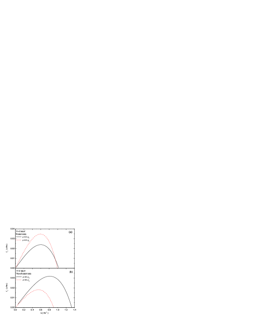
Figure 1: Growth rates of unstable modes as a function of wave numbers in the spinodal region at baryon densities $\rho_{\textrm{b}}=0.2~{}\rho_{0}$ and $\rho_{\textrm{b}}=0.4~{}\rho_{0}$ at temperature $T=5MeV$, (a) relativistic calculations, and (b) non-relativistic calculations.

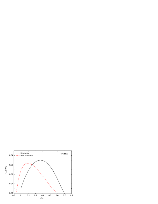
Figure 2: Growth rates of the most unstable modes as function of baryon density in spinodal region at temperature $T=5MeV$ in relativistic calculations (solid line) and in non-relativistic calculations (dashed line).

The evolution in time is determined by taking the inverse Fourier transformation in time, which can be calculated with the help of residue theorem R24 . Keeping only the growing and decaying collective poles, we find,

$$\delta\tilde{\rho}_{\textrm{b}}(\vec{k},t)=\delta\rho_{\textrm{b}}^{+}(\vec{k})e^{+\Gamma_{k}t}+\delta\rho_{\textrm{b}}^{-}(\vec{k})e^{-\Gamma_{k}t}$$ (25)

Here, the amplitudes of baryon density fluctuations associated with the growing and decaying modes at the initial instant are given by,

$$\delta\rho_{\textrm{b}}^{\mp}(\vec{k})=-\left\{\frac{D_{1}\tilde{S}_{\textrm{b}}(\vec{k},\omega)+D_{2}\tilde{S}_{\textrm{s}}(\vec{k},\omega)+D_{3}\tilde{S}_{\textrm{v}}(\vec{k},\omega)}{\partial\varepsilon(\vec{k},\omega)/\partial\omega}\right\}_{\omega=\mp i\Gamma_{k}}$$ (26)

The growth and decay rates of the modes are obtained from the dispersion relations, $\varepsilon(\vec{k},\omega)=0$, i.e. from the roots of susceptibility. Solutions for the scalar density fluctuations $\delta\tilde{\rho}_{\textrm{s}}(\vec{k},\omega)$ and the current density $\delta\tilde{\rho}_{\textrm{v}}(\vec{k},\omega)$ fluctuations can be expressed in a similar manner. In the original Walecka model, there are four free parameters, coupling constants and meson masses. The binding energy per nucleon at saturation density determines the ratios of coupling constants to masses. The standard values of the ratios $g_{\textrm{v}}^{2}(M/m_{\textrm{v}})^{2}=273.8$ and $g_{\textrm{s}}^{2}(M/m_{\textrm{s}})^{2}=357.4$ give binding energy per nucleon $15.75~{}MeV$ at saturation density R13 ; R14 . These ratios lead to an effective nucleon mass $M_{0}^{*}=0.541M$ and a compressibility of $540~{}MeV$ at the saturation density. In numerical calculations, we take for the vector meson mass $m_{\textrm{v}}=783~{}MeV$, and for the scalar meson mass, $m_{\textrm{s}}=500~{}MeV$. As an example, the upper panel in Fig. 1 shows the growth rates of unstable modes as a function of wave number in the spinodal region corresponding to the initial baryon density $\rho_{\textrm{b}}=0.2~{}\rho_{0}$ and $\rho_{\textrm{b}}=0.4~{}\rho_{0}$ at a temperature $T=5~{}MeV$. The lower panel of Fig. 1 illustrates the dispersion relations obtained in the non-relativistic approach with an effective Skyrme force R12 . Although direct comparison of these calculations is rather difficult, we observe there are qualitative differences in both calculations. The range of most unstable modes in relativistic calculations is concentrated around $k=0.6~{}fm^{-1}$ in both densities, while most unstable modes shift towards larger wave numbers around $k=0.8~{}fm^{-1}$ at density $\rho_{\textrm{b}}=0.2~{}\rho_{0}$ towards smaller wave numbers around $k=0.5~{}fm^{-1}$ at density $\rho_{\textrm{b}}=0.4~{}\rho_{0}$. Growth rates of most unstable modes at density $\rho_{\textrm{b}}=0.4~{}\rho_{0}$ in relativistic calculations are nearly factor of two larger than those results obtained in the non-relativistic calculations, while at low density $\rho_{\textrm{b}}=0.2~{}\rho_{0}$ the growth rates are smaller in relativistic calculations. Fig. 2 illustrates growth rates of the most unstable modes as a function of density in both relativistic and non-relativistic approaches. We observe the qualitative difference in the unstable response of the system: the system exhibits most unstable behavior at higher densities around $\rho_{\textrm{b}}=0.4~{}\rho_{0}$ in the relativistic approach while most unstable behavior occurs in the non-relativistic calculations at lower densities around $\rho_{\textrm{b}}=0.2~{}\rho_{0}$. As an example of phase diagrams, Fig. 3 shows the boundary of spinodal region for the unstable mode of wavelength $\lambda=9.0~{}fm$. Again, we observe that the unstable behavior shifts towards higher densities in relativistic calculations.

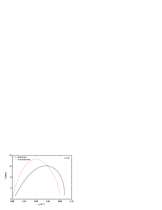
Figure 3: Boundary of spinodal region in baryon density-temperature plane for the unstable mode with wavelengths $\lambda=9~{}fm$ in relativistic calculations (solid line) and in non-relativistic calculations (dashed line).

III.2 Growth of Density fluctuations

In this section, we calculate the early growth of baryon density fluctuations in nuclear matter. Spectral intensity of density correlation function $\tilde{\sigma}_{\textrm{bb}}(\vec{k},t)$ is related to the variance of Fourier transform of baryon density fluctuation according to,

$$\tilde{\sigma}_{\textrm{bb}}(\vec{k},t)(2\pi)^{3}\delta(\vec{k}-\vec{k}^{\prime})=\overline{\delta\tilde{\rho}_{\textrm{b}}(\vec{k},t)\delta\tilde{\rho}_{\textrm{b}}^{*}(\vec{k}^{\prime},t)}$$ (27)

We calculate the spectral function using the solution (25) and the expression (7) for the initial fluctuations to give,

$$\tilde{\sigma}_{\textrm{bb}}(\vec{k},t)=\frac{E_{\textrm{b}}^{+}(\vec{k})}{|[\partial\epsilon(\vec{k},\omega)/\partial\omega]_{\omega=i\Gamma_{k}}|^{2}}(e^{2\Gamma_{k}t}+e^{-2\Gamma_{k}t})+\frac{2E_{\textrm{b}}^{-}(\vec{k})}{|[\partial\epsilon(\vec{k},\omega)/\partial\omega]_{\omega=i\Gamma_{k}}|^{2}}$$ (28)

where

$$E_{\textrm{b}}^{\mp}(\vec{k}) = |D_{1}|^{2}K_{11}^{\mp}+|D_{2}|^{2}K_{22}^{\mp}\mp|D_{3}|^{2}K_{33}^{\mp}+2D_{1}D_{2}K_{12}^{\mp}$$ (29)

with

$$K_{11}^{\mp}=\gamma^{2}\int\frac{d^{3}p}{(2\pi)^{3}}\frac{\Gamma_{k}^{2}\mp(\vec{\textrm{v}}_{0}\cdot\vec{k})^{2}}{[\Gamma_{k}^{2}+(\vec{\textrm{v}}_{0}\cdot\vec{k})^{2}]^{2}}f_{0}(p)[1-f_{0}(p)],$$ (30)

$$K_{22}^{\mp}=\gamma^{2}\int\frac{d^{3}p}{(2\pi)^{3}}\left(\frac{M_{0}^{*}}{e^{*}_{0}}\right)^{2}\frac{\Gamma_{k}^{2}\mp(\vec{\textrm{v}}_{0}\cdot\vec{k})^{2}}{[\Gamma_{k}^{2}+(\vec{\textrm{v}}_{0}\cdot\vec{k})^{2}]^{2}}f_{0}(p)[1-f_{0}(p)],$$ (31)

$$K_{33}^{\mp}=\gamma^{2}\int\frac{d^{3}p}{(2\pi)^{3}}\left(\frac{\vec{p}\cdot\vec{k}}{e^{*}_{0}}\right)^{2}\frac{\Gamma_{k}^{2}\mp(\vec{\textrm{v}}_{0}\cdot\vec{k})^{2}}{[\Gamma_{k}^{2}+(\vec{\textrm{v}}_{0}\cdot\vec{k})^{2}]^{2}}f_{0}(p)[1-f_{0}(p)],$$ (32)

and

$$K_{12}^{\mp}=\gamma^{2}\int\frac{d^{3}p}{(2\pi)^{3}}\frac{M_{0}^{*}}{e^{*}_{0}}\frac{\Gamma_{k}^{2}\mp(\vec{\textrm{v}}_{0}\cdot\vec{k})^{2}}{[\Gamma_{k}^{2}+(\vec{\textrm{v}}_{0}\cdot\vec{k})^{2}]^{2}}f_{0}(p)[1-f_{0}(p)].$$ (33)

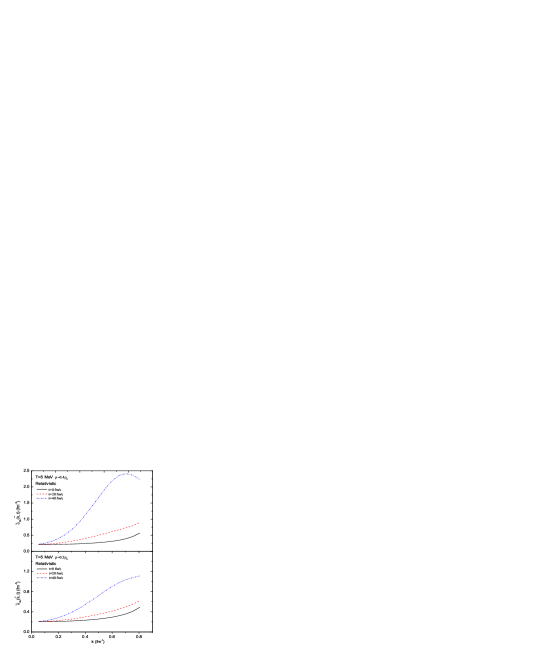
Figure 4: Spectral intensity $\tilde{\sigma}_{\textrm{b}}(\vec{k},t)$ of baryon density correlation function as a function of wave number at times $t=0$, $t=20~{}fm/c$ and $t=40~{}fm/c$ at temperature $T=5~{}MeV$ in relativistic calculations at density (a) $\rho_{\textrm{b}}=0.2~{}\rho_{0}$ and (b) $\rho_{\textrm{b}}=0.4~{}\rho_{0}$.

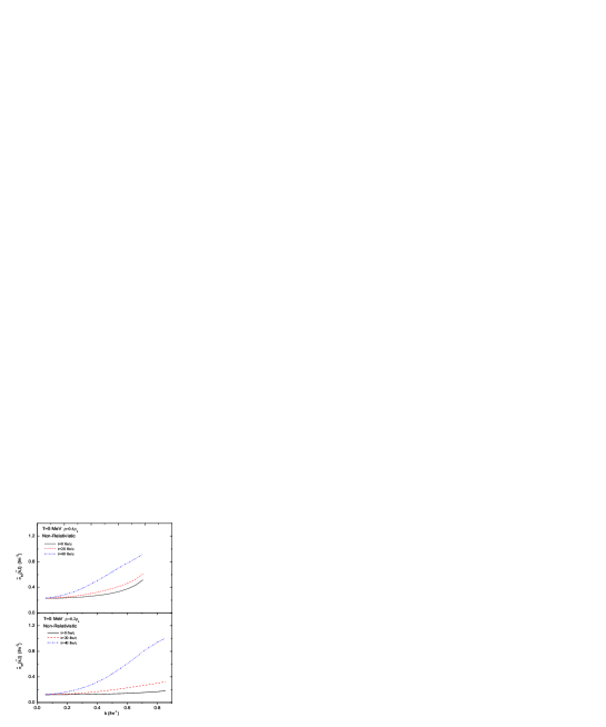
Figure 5: Same as figure 4 in non-relativistic calculations.

Upper and lower panels of Fig. 4 show the spectral intensity of the baryon density correlation function as a function of wave number at times $t=0$, $t=20~{}fm/c$ and $t=40~{}fm/c$ at temperature $T=5~{}MeV$ in relativistic calculations at densities $\rho_{\textrm{b}}=0.2~{}\rho_{0}$ and $\rho_{\textrm{b}}=0.4~{}\rho_{0}$, respectively. We observe that the largest growth occurs over the range of wave numbers corresponding to the range of dominant unstable modes. Spectral intensity in the vicinity of most unstable modes of $k=0.6~{}fm^{-1}$ grows about a factor of ten at density $\rho_{\textrm{b}}=0.2~{}\rho_{0}$ and about a factor of six at density $\rho_{\textrm{b}}=0.4~{}\rho_{0}$ during the time interval of $t=40~{}fm/c$. Fig. 5 shows the similar information calculated in non-relativistic approaches. We notice that at density $\rho_{\textrm{b}}=0.2~{}\rho_{0}$ the behavior of spectral intensity is rather similar in relativistic and non-relativistic approache. However, at higher density $\rho_{\textrm{b}}=0.4~{}\rho_{0}$, the spectral intensity grows slower in the non-relativistic calculations than those obtained in the relativistic approach. We note that in determining time evolution $\delta\rho_{\textrm{b}}(\vec{k},t)$ with the help of the residue theorem, there are other contributions arising form the non-collective pole of the susceptibility $\varepsilon(\vec{k},\omega)$ and from the poles of source terms $\tilde{S}_{\textrm{v}}(\vec{k},\omega)$, $\tilde{S}_{\textrm{s}}(\vec{k},\omega)$ and $\tilde{S}_{\textrm{b}}(\vec{k},\omega)$. These contributions, in particular towards the short wavelengths, i.e. towards higher wave numbers, are important at the initial stage, however they damp out in a short time interval R25 . Since, we do not include effects from non-collective poles, we terminate the spectral in Fig. 5 at a cut-off wave number $k_{c}~{}\approx~{}0.7~{}fm^{-1}~{}-~{}0.8~{}fm^{-1}$. Consequently, the expression (28) provides a good approximation for $\tilde{\sigma}_{bb}(\vec{k},t)$ in the long wavelength regime below $k_{c}$.

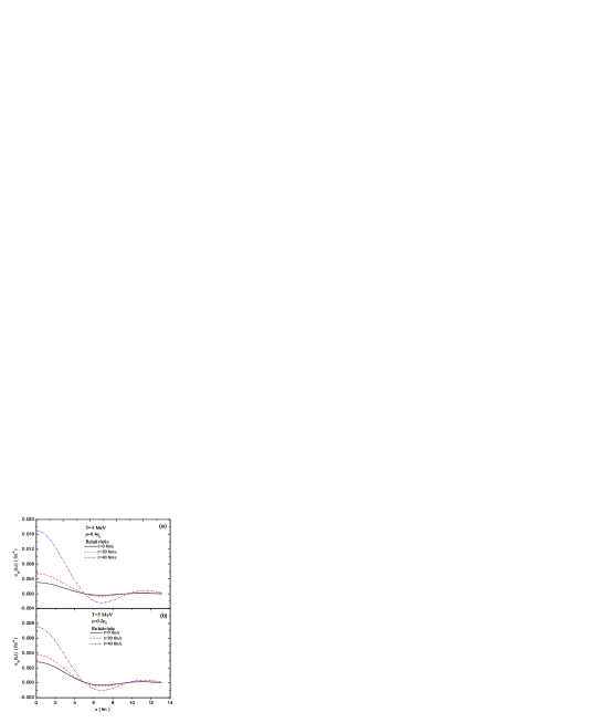
Figure 6: Baryon density correlation function $\sigma_{\textrm{b}}(x,t)$ as a function of distance $x=|\vec{r}-\vec{r}^{\prime}|$ between two space points at times $t=0$, $t=20~{}fm/c$ and $t=40~{}fm/c$ at temperature $T=~{}5$ MeV in relativistic calculations at density (a) $\rho_{\textrm{b}}=0.2~{}\rho_{0}$ and (b) $\rho_{\textrm{b}}=0.4~{}\rho_{0}$.

Local baryon density fluctuations $\delta\rho_{\textrm{b}}(\vec{r},t)$ are determined by the Fourier transform of $\delta\rho_{\textrm{b}}(\vec{k},t)$. Equal time correlation function of baryon density fluctuations as a function of distance between two space locations can be expressed in terms of the spectral intensity as,

$$\sigma_{\textrm{bb}}(|\vec{r}-\vec{r}^{\prime}|,t)=\overline{\delta n{\textrm{b}}(\vec{r},t)\delta n_{\textrm{b}}(\vec{r}^{\prime},t)}=\int\frac{d^{3}k}{(2\pi)^{3}}e^{i\vec{k}\cdot\vec{r}}\tilde{\sigma}_{\textrm{bb}}(\vec{k},t).$$ (34)

The baryon density correlation function carries useful information about the unstable dynamics of the matter in the spinodal region. As an example, the upper and lower panels of Fig. 6 illustrates the baryon density correlation function as a function distance between two space points at times $t=0$, $t=20~{}fm/c$, and $t=40~{}fm/c$ at temperature $T=~{}5$ MeV in relativistic calculations at densities $\rho_{\textrm{b}}=0.4~{}\rho_{0}$ and $\rho_{\textrm{b}}=0.2~{}\rho_{0}$, respectively. Complementary to the dispersion relation, correlation length of baryon density fluctuations provides an additional measure for the size of the primary fragmentation pattern. We can estimate the correlations length of baryon density fluctuations as the width of the correlation function at at half maximum. From the figure, we estimate that the correlation length is about the same at both densities and temperatures around $3.0~{}fm$, which is consistent with the dispersion relation presented in Fig. 1. Baryon density fluctuations grow faster at $\rho_{\textrm{b}}=0.4~{}\rho_{0}$ than $\rho_{\textrm{b}}=0.2~{}\rho_{0}$. Fig. 7 shows the similar information calculated in the non-relativistic approach R12 . The correlation length is around $3.0~{}fm$ at $\rho_{\textrm{b}}=0.4~{}\rho_{0}$ and $3.0~{}fm$ at the lower density $\rho_{\textrm{b}}=0.2~{}\rho_{0}$. However, unlike the relativistic calculations, the baryon density fluctuations grow faster at lower density $\rho_{\textrm{b}}=0.2~{}\rho_{0}$ than at $\rho_{\textrm{b}}=0.4~{}\rho_{0}$, which is consistent result presented in Fig. 2.

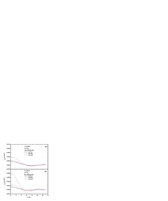
Figure 7: Same as figure 6 in non-relativistic calculations.

IV CONCLUSIONS

It has been demonstrated in recent publications R7 ; R9 ; R10 ; R12 that the stochastic mean-field approach incorporates both the one-body dissipation and the associated fluctuation mechanism in a manner consistent with the fluctuation-dissipation theorem of non-equilibrium statistical mechanics. Therefore the approach provides a powerful tool for investigating dynamics of density fluctuations in low-energy nuclear collisions. In a similar manner, it is possible to develop an extension of the relativistic mean-field theory by incorporating the initial quantal zero point fluctuations and thermal fluctuations of density in a stochastic manner. In this work, by employing the stochastic extension of the relativistic mean-field approach, we investigate spinodal instabilities in symmetric nuclear matter in the semi-classical framework. We determine the growth rates of unstable collective modes at different initial densities and temperatures. Stochastic approach also allows us to calculate early development of baryon density correlation functions in spinodal region, which provides valuable complementary information about the emerging fragmentation pattern of the system. We compare the results with those obtained in non-relativistic calculations under similar conditions. Our calculations indicate a qualitative difference in behavior in the unstable response of the system. In the relativistic approach, the system exhibits most unstable behavior at higher baryon densities around $\rho_{\textrm{b}}=0.4~{}\rho_{0}$, while in the non-relativistic calculations most unstable behavior occurs at lower baryon densities around $\rho_{\textrm{b}}=0.2~{}\rho_{0}$. In the present exploratory work, we employ the original Walacka model without self-interaction of scalar meson. The qualitative difference in the unstable behavior may be partly due to the fact that the original Walecka model leads to a relatively small value of nucleon effective mass of $M^{*}=0.541M$ and a large nuclear compressibility of $540~{}MeV$. On the other hand, the Skyrme interaction that we employ in non-relativistic calculations gives rise to a compressibility of $201~{}MeV$ R12 . It will be interesting to carry out further investigations of spinodal dynamics in symmetric and charge asymmetric nuclear matter by including self-interaction of the scalar meson and also including the rho meson in the calculations. Inclusion of the self-interaction of scalar meson allows us to investigate spinodal dynamics over a wide range of nuclear compressibility and nuclear effective mass. We also note by working in the semi-classical framework, we neglect the quantum statistical effects on the baryon density correlation function, which become important at lower temperatures and also at lower densities.

References

• (1) Ph. Chomaz, M. Colonna and J. Randrup, Phys. Rep. 389 (2004) 263.
• (2) S. Ayik, M. Colonna and Ph. Chomaz, Phys. Lett. B353 (1995) 417.
• (3) B. Jacquot, S. Ayik, Ph. Chomaz and M. Colonna, Phys. Lett. B383 (1996) 247.
• (4) B. Jacquot, M. Colonna, S. Ayik and Ph. Chomaz, Nucl. Phys. A617 (1997) 356.
• (5) M. Colonna, Ph. Chomaz and S. Ayik, Phys. Rev. Lett. 88 (2002) 122701.
• (6) V. Baran, M. Colonna, M. Di Tora and A. B. Larionov, Nucl. Phys. A632 (1998) 287.
• (7) S. Ayik, Phys. Lett. B 658 (2008) 174.
• (8) R. Balian and M. Veneroni, Phys. Lett. B 104 (1982) 121.
• (9) S. Ayik, K. Washiyama and D. Lacroix, Phys. Rev. C 79 (2009) 0546606.
• (10) K. Washiyama, S. Ayik and D. Lacroix, submitted to Phys. Rev. Lett. (2009)
• (11) H. Feldmeier, Rep. Prog. Phys. 50 (1987) 915
• (12) S. Ayik, N. Er, O. Yilmaz and A. Gokalp, Nucl. Phys. A 812 (2008) 44.
• (13) P. Ring, Prog. Part. Nucl. Phys. 37 (1996) 193.
• (14) B. D. Serot and J. D. Walecka, Int. J. Mod. Phys. E 6 (1997) 515.
• (15) D. Vretenar, H. Berghammer and P. Ring, Nucl. Phys. A 581 (1995) 679.
• (16) D. Vretenar, A. V. Afanasjev, G. A. Lalazissis and P. Ring, Phys. Rep. 409 (2005) 101.
• (17) S. S. Avancini, L. Brito, D. P. Menezes and C. Providencia, Phys. Rev. C 71 (2005) 044323.
• (18) A. M. Santos, L. Brito and C. Providencia, Phys. Rev. C 77 (2008) 045805.
• (19) C. Ducoin, C. Providencia , A. M. Santos, L. Brito and Ph. Chomaz, Phys. Rev. C 78 (2005) 055801.
• (20) C. H. Dasso, T. Dossing, and H. C. Pauli, Z. Phys. A 289 (1979) 395 .
• (21) H. Esbensen, A. Winther, R. A. Broglia, and C. H. Dasso, Phys. Rev. Lett. 41 (1978) 296.
• (22) C. H. Dasso, Proc. Second La Rapida Summer School on Nuclear Physics, eds. M. Lozano and G. Madurga, World Scientific, Singapore, 1985.
• (23) C. M. Ko, Q. Li and R. Wang, Phys. Rev. Lett. 59 (1987) 1084
• (24) E. M. Lifshitz and P.L. Pitaevskii, ”Physical Kinetics”, Pergamon, 1981.
• (25) P. Bozek, Phys. Lett. B 383 (1996) 121.