Branes in the $M_{D}\times M_{d^{+}}\times M_{d^{-}}$ Compactification of type II string on $S^{1}/Z_{2}$ and their cosmological applications

Abstract

In this paper, we study the implementation of brane worlds in type II string theory. Starting with the NS/NS sector of type II string, we first compactify the $\left(D+d_{+}+d_{-}\right)$-dimensional spacetime, and reduce the corresponding action to a D-dimensional effective action, where the topologies of $M_{d_{+}}$ and $M_{d_{-}}$ are arbitrary. We further compactify one of the $(D-1)$ spatial dimensions on an $S^{1}/Z_{2}$ orbifold, and derive the gravitational and matter field equations both in the bulk and on the branes. Then, we investigate two key issues in such a setup: (i) the radion stability and radion mass; and (ii) the localization of gravity, and the corresponding Kaluza-Klein (KK) modes. We show explicitly that the radion is stable and its mass can be in the order of $GeV$. In addition, the gravity is localized on the visible brane, and its spectrum of the gravitational KK towers is discrete and can have a mass gap of $TeV$, too. The high order Yukawa corrections to the 4-dimensional Newtonian potential is exponentially suppressed, and can be negligible. Applying such a setup to cosmology, we obtain explicitly the field equations in the bulk and the generalized Friedmann equations on the branes.

I Introduction

Brane worlds have been studied extensively in the past decade branes , following Horava and Witten’s (HW) ideas HW96 , where gauge fields of the standard model (SM) are confined on two 9-branes located at the end points of an $S^{1}/Z_{2}$ orbifold. Out of the 9-spatial dimensions of the branes, six are compactified on a very small scale close to the fundamental one. A 5-dimensional effective theory of the 11-dimensional HW heterotic M-Theory on $S^{1}/Z_{2}$ was worked out explicitly by Lukas et al LOSW99 , and shown that the radion is stable LSS05 ; WGW08 , and its mass is of the order of $0.1\;GeV$ WGW08 . In addition, the corresponding tensor perturbations were also studied, and found that the gravity is localized in the visible (TeV) brane WGW08 . The spectrum of the gravitational Kaluza-Klein (KK) towers is discrete, and the mass gap can be in the order of $TeV$. The corrections to the 4-dimensional Newtonian potential, due to the high order KK modes, are exponentially suppressed, and are consistent with observations WGW08 . In such a setup, the long standing hierarchy problem, namely the large difference in magnitudes between the Planck and electroweak scales, may be potentially resolved by combining the large extra dimension ADD98 , warped-factor RS1 and brane-tension coupling Cline99 mechanisms. One of the most attractive features of the model, similar to the RS1 model RS1 , is that it might be soon explored by LHC DHR00 . For critical reviews of the brane worlds and some open issues, we refer readers to branes .

Another important application of brane worlds is to the cosmological constant problem wen . In the 4-dimensional spacetimes, there exists Weinberg’s no-go theorem for the adjustment of the cosmological constant. However, in higher dimensional spacetimes, the 4-dimensional vacuum energy on the brane does not necessarily give rise to an effective 4-dimensional cosmological constant. Instead, it may only curve the bulk, while leaving the brane still flat CEG01 , whereby Weinberg’s no-go theorem is evaded. Along this vein, the cosmological constant problem was studied in the framework of brane worlds in 5-dimensional spacetimes 5CC and 6-dimensional supergravity 6CC . However, it was soon realized that in the 5-dimensional case hidden fine-tunings are required For00 . In the 6-dimensional case such fine-tunings may not be needed, but it is still not clear whether loop corrections can be as small as expected Burg07 .

In addition, by adding an Einstein-Hilbert term to the brane action, Dvali, Gabadadze and Porrati (DGP) DGP showed that gravity can be altered at immense distances, due to the slow leakage of gravity off our 3-dimensional universe into bulk. It should be noted that the DGP model has only one 3-brane, and the spacetime in the direction perpendicular to the brane is usually infinitely large, in contrast to the RS1 model, where two orbifold branes form the boundary in the transverse direction of the branes, although later Randall and Sundrum proposed another model (RS2), in which only one brane exists RS2 . A remarkable feature of the DGP model is that it gives rise to a late cosmic acceleration of the universe, without the introduction of dark energy Def . It must be noted that, despite of this great success, the DGP model, as well as its hybrids, is usually plagued with the problem of ghost ghost1 ; ghost2 , in addition to the problem of the consistency with observations Hu08 ; GIW09 .

It should also be noted that the RS1, RS2 and DGP brane worlds, as well as their generalizations branes , are phenomenological models, and how to implement them into string/M theory is still an open question, despite of some important efforts along this direction Ben99 ; Chen06 . Such an implementation turns out to be extremely difficult, as one would expect, given the complexity of the theory. It was exactly because of this that most of the previous works on brane worlds are phenomenological, and should be considered only as an intermediary bridge between observations and fundamental theory.

Lately, as part of the efforts of implementing the RS1 model into string/M theory, the orbifold branes and their applications to cosmology were studied systematically in the framework of both the Horava-Witten heterotic M-Theory GWW07 ; WGW08 and string theory WS07 ; WSVW08 ; WS08 on $S^{1}/Z_{2}$. From the point of view of pure numerology, it was found that the 4D effective cosmological constant can be cast in the form,

$$\rho_{\Lambda}=\frac{\Lambda_{4}}{8\pi G_{4}}=3\left(\frac{R}{l_{pl}}\right)^{\alpha_{R}}\left(\frac{M}{M_{pl}}\right)^{\alpha_{M}}M_{pl}^{4},$$ (1.1)

where $R$ denotes the typical size of the extra dimensions, $M$ the energy scale of string or M theory, and $(\alpha_{R},\alpha_{M})=(10,16)$ for string theory WS07 and $(\alpha_{R},\alpha_{M})=(12,18)$ for the HW heterotic M Theory GWW07 . In both cases, it can be shown that for $R\simeq 10^{-22}\;m$ and $M\simeq 1\;TeV$, we obtain $\rho_{\Lambda}\sim\rho_{\Lambda,ob}\simeq 10^{-47}\;GeV^{4}$. In contrast to that in Einstein’s theory, the domination of this term is only temporary. Due to the interaction of the bulk and the brane, the universe will be in its decelerating expansion phase again, whereby all problems connected with a far future de Sitter universe Fish ; KS00 are resolved. This feature was also found in the DGP model DGP . Therefore, a late transient acceleration of the universe seems to be a generic feature of brane worlds.

It was also showed that the radion is stable, and its mass is about $10^{-1}$ GeV in the Horava-Witten heterotic M-Theory WGW08 and $10^{-2}$ GeV in the string theory WS08 . The gravity is localized on the visible (TeV) brane. The spectrum of the gravitational KK towers is discrete with a mass gap that can be in the order of TeV. The high order Yukawa corrections to the 4-dimensional effective Newtonian potential are exponentially suppressed.

In this paper, we shall continuously work along the direction of implementing the RS1 model RS1 into string/M theory. In particular, In Sec. II, starting with the Neveu-Schwarz/Neveu-Schwarz (NS/NS) sector of type II string, we first consider the compactification of the $\left(D+d_{+}+d_{-}\right)$-dimensional spacetime on two manifolds $M_{d_{+}}$ and $M_{d_{-}}$, where the topologies of $M_{d_{+}}$ and $M_{d_{-}}$ are unspecified. This opens the possibility of having the dilaton and modulus fields non-zero potentials (masses), which is in contrast to the toroidal compactification considered in WS07 ; WSVW08 ; WS08 , in which these scalar fields are always massless LWC00 ; BW06 ; TW09 . After reducing the action to an effective $D$-dimensional one, we further compactify one of the $(D-1)$ spatial dimensions on an $S^{1}/Z_{2}$ orbifold. Lifting it to the original spacetime, they represent $(D+d_{+}+d_{-}-2)$-dimensional orbiford branes. The corresponding gravitational and matter field equations both in the bulk and on the branes are derived separately in Sec. III, while in Sec. IV such developed formulas are applied to cosmology by setting $D=5=d_{+}+d_{-}$. In particular, the generalized Friedmann equations are given explicitly on the branes. In Sec. V the radion stability and radion mass are studied, while in Sec. VI, the tensor perturbations are investigated. It is found that the radion stable, and the gravity is localized on the visible brane. Both the radion mass and the mass gap of the gravitational KK towers can be in the order of $TeV$, by properly choosing the free parameters presented in the model. The high order Yukawa corrections to the 4-dimensional Newtonian potential, due to the high order KK modes, is exponentially suppressed, and can be negligible. The paper is ended with Sec. VII, in which we summarize our main results and present some remarks to the future work.

To have this paper as much independent as possible, for the sake of reader’s convenience, some parts might be repeated from our previous studies of the problems, although we try to limit these to their minimum.

Before proceeding further, we would like to note that, to have a late time accelerating universe from string/M-Theory, Townsend and Wohlfarth townsend invoked a time-dependent compactification of pure gravity in higher dimensions with hyperbolic internal space to circumvent Gibbons’ non-go theorem gibbons . Their exact solution exhibits a short period of acceleration. The solution is the zero-flux limit of spacelike branes ohta . If non-zero flux or forms are turned on, a transient acceleration exists for both compact internal hyperbolic and flat spaces wohlfarth . Other accelerating solutions by compactifying more complicated time-dependent internal spaces can be found in string .

II The Model

In this section, we consider the compactification of the NS/NS sector in ($D+d_{+}+d_{-}$)-dimensions, and obtain an effective $D$-dimensional action. Then, we compactify one of the $(D-1)$ spatial dimensions by introducing two orbifold branes as the boundaries along this compactified dimension.

II.1 Compactification of the NS/NS sector

Let us consider the NS/NS sector in ($D+d_{+}+d_{-}$)-dimensions, $\hat{M}_{N}=M_{D}\times{\cal{M}}_{d_{+}}\times{\cal{M}}_{d_{-}}$, where ${\cal{M}}_{d_{+}}$ and ${\cal{M}}_{d_{-}}$ are $d_{+}$ and $d_{-}$ dimensional spaces, respectively, and $N\equiv D+d_{+}+d_{-}$. To have our formulas as much applicable as possible, we shall not specify the topologies of these spaces. The action takes the form LWC00 ; BW06 ; MG07 ,

$$\hat{S}_{N} = -\frac{1}{2\kappa^{2}_{N}}\int{d^{N}x\sqrt{\left|\hat{g}_{N}\right|}e^{-\hat{\Phi}}}$$ (2.1)

$$\times\left\{{\hat{R}}_{N}[\hat{g}]+\left(\hat{\nabla}\hat{\Phi}\right)^{2}-\frac{1}{12}{\hat{H}}^{2}\right\},\;\;\;$$

where $\hat{\nabla}$ denotes the covariant derivative with respect to $\hat{g}^{AB}$ with $A,B=0,1,...,N-1$, and $\hat{\Phi}$ is the dilaton field. The NS three-form field $\hat{H}_{ABC}$ is defined as

$$\hat{H}_{ABC} = 3\partial_{[A}\hat{B}_{BC]}$$ (2.2)

$$= \partial_{A}\hat{B}_{BC}+\partial_{B}\hat{B}_{CA}+\partial_{C}\hat{B}_{AB},$$

where the square brackets imply total antisymmetrization over all indices, and

$$\hat{B}_{CD}=-\hat{B}_{DC},\;\;\;\partial_{A}\hat{B}_{CD}\equiv\frac{\partial\hat{B}_{CD}}{\partial{x^{A}}}.$$ (2.3)

The constant $\kappa^{2}_{N}$ denotes the gravitational coupling constant, defined as

$$\kappa^{2}_{N}=8\pi G_{N}=\frac{1}{M_{N}^{N-2}},$$ (2.4)

where $G_{N}$ and $M_{N}$ denote, respectively, the $N$-dimensional Newtonian constant and Planck mass.

In this paper we consider the $N$-dimensional spacetimes described by the metric,

$$d{\hat{s}}^{2}_{N} = \hat{g}_{AB}dx^{A}dx^{B}$$ (2.5)

$$= \tilde{g}_{ab}\left(x\right)dx^{a}dx^{b}+e^{\sqrt{\frac{2}{d_{+}}}\psi_{+}(x)}h^{+}_{ij}\left(z_{+}\right)dz^{i}_{+}dz^{j}_{+}$$

$$+e^{\sqrt{\frac{2}{d_{-}}}\psi_{-}(x)}h^{-}_{pq}\left(z_{-}\right)dz_{-}^{p}dz_{-}^{q},$$

where $\tilde{g}_{ab}(x)$ is the metric on $M_{D}$, parametrized by the coordinates $x^{a}$ with $a,b,c=0,1,...,D-1$, $h^{+}_{ij}\left(z_{+}\right)$ the metric on the compact space ${\cal{M}}_{d_{+}}$ with coordinates $z_{+}^{i}$, where $i,j=D,D+1,...,D+d_{+}-1$, and $h^{-}_{ij}\left(z_{-}\right)$ the metric on the compact space ${\cal{M}}_{d_{-}}$ with coordinates $z_{-}^{p}$, where $p,q=D+d_{+},D+d_{+}+1,...,N-1$.

We assume that the daliton field $\hat{\Phi}$ is function of $x^{a}$, and the flux $\hat{B}_{CD}$ is block diagonal,

$$\left(\hat{B}_{CD}\right) = \left(\matrix{{B}_{ab}(x)&0&0\cr 0&e^{\xi_{+}(x)}B_{ij}\left(z_{+}\right)&0\cr 0&0&e^{\xi_{-}(x)}B_{pq}\left(z_{-}\right)}\right).$$

Then, it can be shown that the non-vanishing components of $\hat{H}_{ABC}$ are

$$\hat{H}_{abc} = {H}_{abc}=3\partial_{[a}{B}_{bc]},$$

$$\hat{H}_{ijk} = e^{\xi_{+}}H_{ijk}=3e^{\xi_{+}}\partial_{[i}{B}_{jk]},$$

$$\hat{H}_{pqr} = e^{\xi_{-}}H_{pqr}=3e^{\xi_{-}}\partial_{[p}{B}_{qr]},$$

$$\hat{H}_{aij} = B_{ij}e^{\xi_{+}}\tilde{\nabla}_{a}{\xi_{+}},$$

$$\hat{H}_{apq} = B_{pq}e^{\xi_{-}}\tilde{\nabla}_{a}{\xi_{-}},$$ (2.7)

where $\tilde{\nabla}_{a}$ denotes the covariant derivative with respect to $\tilde{g}^{ab}$. On the other hand, we also have

$${\hat{R}}_{N}[\hat{g}] = \tilde{R}_{D}[\tilde{g}]+e^{-\sqrt{\frac{2}{d_{+}}}\psi_{+}}R_{d_{+}}\left[h^{+}\right]$$ (2.8)

$$+e^{-\sqrt{\frac{2}{d_{-}}}\psi_{-}}R_{d_{-}}\left[h^{-}\right]$$

$$-2\tilde{g}^{ab}\tilde{\nabla}_{a}\tilde{\nabla}_{b}Q-\frac{(d_{+}+1)}{2}\left(\tilde{\nabla}\psi_{+}\right)^{2}$$

$$-\frac{(d_{-}+1)}{2}\left(\tilde{\nabla}\psi_{-}\right)^{2}$$

$$-\sqrt{d_{+}d_{-}}\left(\tilde{\nabla}\psi_{+}\right)\left(\tilde{\nabla}\psi_{-}\right),$$

where

$$Q\equiv\sqrt{\frac{d_{+}}{2}}\;\psi_{+}+\sqrt{\frac{d_{-}}{2}}\;\psi_{-}.$$ (2.9)

Making the following conformal transformations,

$$g_{ab}=\Omega^{2}\tilde{g}_{ab},\;\;\;\Omega=e^{\frac{Q-\hat{\Phi}}{D-2}},$$ (2.10)

we find that

$$\tilde{R}_{D}[\tilde{g}] = \Omega^{2}\left\{R_{D}[g]+2(D-1)\Box\ln\Omega\right.$$

$$\left.-(D-2)(D-1)\left(\nabla\ln\Omega\right)^{2}\right\},$$

$$\tilde{g}^{ab}\tilde{\nabla}_{a}\tilde{\nabla}_{b}Q = \Omega^{2}\left(\Box{Q}\right.$$ (2.11)

$$\left.-(D-2)\left(\nabla{Q}\right)\left(\nabla\ln\Omega\right)\right),$$

where $\Box\equiv g^{ab}\nabla_{a}\nabla_{b}$, and ${\nabla}_{a}$ denotes the covariant derivative with respect to ${g}^{ab}$. Then, combining Eqs.(2.8) and (II.1), we obtain

$$\sqrt{\left|\hat{g}_{N}\right|}e^{-\hat{\Phi}}\left\{{\hat{R}}_{N}[\hat{g}]+\left(\hat{\nabla}\hat{\Phi}\right)^{2}-\frac{1}{12}{\hat{H}}^{2}\right\}$$

$$=\sqrt{\left|{g}_{D}{h^{+}}{h^{-}}\right|}\left\{R_{D}[g]+e^{-2\frac{Q-\hat{\Phi}}{D-2}}\left(e^{-\sqrt{\frac{2}{d_{+}}}\psi_{+}}R_{d_{+}}\right.\right.$$

$$\left.+e^{-\sqrt{\frac{2}{d_{-}}}\psi_{-}}R_{d_{-}}-\frac{1}{12}{\hat{H}}^{2}\right)+\frac{2}{D-2}\Box{Q}$$

$$-\frac{2(D-1)}{D-2}\Box{\hat{\Phi}}-\frac{1}{D-2}\left(\nabla{\left(Q-\hat{\Phi}\right)}\right)^{2}$$

$$\left.-\frac{1}{2}\left(\nabla\psi_{+}\right)^{2}-\frac{1}{2}\left(\nabla\psi_{-}\right)^{2}\right\},$$ (2.12)

where

$$\hat{H}^{2} = e^{\frac{6\left(Q-\hat{\Phi}\right)}{D-2}}H^{2}$$ (2.13)

$$+3e^{\frac{2\left(Q-\hat{\Phi}\right)}{D-2}}\left(e^{2\left(\xi_{+}-\sqrt{\frac{2}{d_{+}}}\psi_{+}\right)}B_{+}^{2}\left(\nabla\xi_{+}\right)^{2}\right.$$

$$\left.+e^{2\left(\xi_{-}-\sqrt{\frac{2}{d_{-}}}\psi_{-}\right)}B_{-}^{2}\left(\nabla\xi_{-}\right)^{2}\right)$$

$$+e^{2\xi_{+}-3\sqrt{\frac{2}{d_{+}}}\psi_{+}}H^{2}_{+}$$

$$+e^{2\xi_{-}-3\sqrt{\frac{2}{d_{-}}}\psi_{-}}H^{2}_{-},$$

with

$$H^{2} = H_{abc}(x)H^{abc}(x),$$

$$H^{2}_{+} = H_{ijk}\left(z_{+}\right)H^{ijk}\left(z_{+}\right),$$

$$H^{2}_{-} = H_{pqr}\left(z_{-}\right)H^{pqr}\left(z_{-}\right),$$

$$B^{2}_{+} = B_{ij}\left(z_{+}\right)B^{ij}\left(z_{+}\right),$$

$$B^{2}_{-} = B_{pq}\left(z_{-}\right)B^{pq}\left(z_{-}\right),$$ (2.14)

and

$$g^{ab}g_{ac}=\delta^{b}_{c},\;\;\;h^{+ik}h^{+}_{ij}=\delta^{k}_{j},\;\;\;h^{-pq}h^{-}_{pr}=\delta^{q}_{r}.$$ (2.15)

Substituting Eqs.(2.13) and (II.1) into Eq.(2.1), and then integrating it by part, we obtain the $D-$dimensional effective action in the Einstein frame,

$$S_{D}^{(E)}=-\frac{1}{2\kappa_{D}^{2}}\int{\sqrt{\left|g_{D}\right|}d^{D}x\left(R_{D}[g]-{\cal{L}}^{(E)}_{D}\left(\phi_{n},\xi_{\pm}\right)\right)},$$ (2.16)

where $\phi_{n}=\left\{\phi,\psi_{\pm}\right\}$, and

$$\kappa_{D}^{2} \equiv \frac{\kappa_{N}^{2}}{V_{d_{+}}V_{d_{-}}},$$ (2.17)

$$V_{d_{\pm}} \equiv \int{\sqrt{\left|h^{\pm}\right|}\;d^{d_{\pm}}z_{\pm}},$$

$${\cal{L}}^{(E)}_{D} = \frac{1}{2}\sum_{n}{\left(\nabla\phi_{n}\right)^{2}}+\frac{1}{12}e^{-\sqrt{\frac{8}{D-2}}\phi}H^{2}$$ (2.18)

$$+\alpha_{+}e^{2\xi_{+}-\sqrt{\frac{8}{{d_{+}}}}\psi_{+}}\left(\nabla\xi_{+}\right)^{2}$$

$$+\alpha_{-}e^{2\xi_{-}-\sqrt{\frac{8}{{d_{-}}}}\psi_{-}}\left(\nabla\xi_{-}\right)^{2}$$

$$-e^{\sqrt{\frac{2}{D-2}}\phi}\left(\beta_{+}e^{-\sqrt{\frac{2}{d_{+}}}\psi_{+}}\right.$$

$$+\beta_{-}e^{-\sqrt{\frac{2}{d_{-}}}\psi_{-}}-\gamma_{+}e^{2\xi_{+}-\sqrt{\frac{18}{{d_{+}}}}\psi_{+}}$$

$$\left.-\gamma_{-}e^{2\xi_{-}-\sqrt{\frac{18}{d_{-}}}\psi_{-}}\right),\;\;$$

and

$$\phi \equiv \sqrt{\frac{2}{D-2}}\left(\hat{\Phi}-Q\right),$$ (2.19)

$$\alpha_{\pm} \equiv \frac{1}{4V_{d_{\pm}}}\int{d^{d_{\pm}}z_{\pm}\;\sqrt{\left|h^{\pm}\right|}B^{2}_{\pm}\left(z_{\pm}\right)},$$

$$\beta_{\pm} \equiv \frac{1}{V_{d_{\pm}}}\int{d^{d_{\pm}}z_{\pm}\;\sqrt{\left|h^{\pm}\right|}R_{d_{\pm}}\left(z_{\pm}\right)},$$

$$\gamma_{\pm} \equiv \frac{1}{12V_{d_{\pm}}}\int{d^{d_{\pm}}z_{\pm}\;\sqrt{\left|h^{\pm}\right|}H^{2}_{\pm}\left(z_{\pm}\right)}.$$ (2.20)

II.2 $S^{1}/Z_{2}$ Compactification of the D-Dimensional Sector

We shall compactify one of the $(D-1)$ spatial dimensions by placing two orbifold branes as its boundaries. The brane actions are taken as,

$$S^{(E,I)}_{D-1,m} = -\epsilon_{I}\int_{M^{(I)}_{D-1}}{\sqrt{\left|g^{(I)}_{D-1}\right|}V^{(I)}_{D-1}\left(\phi_{n},\xi_{\pm}\right)d^{D-1}\xi_{(I)}}$$ (2.21)

$$+\int_{M^{(I)}_{D-1}}{d^{D-1}\xi_{(I)}\sqrt{\left|g^{(I)}_{D-1}\right|}}$$

$$\times{\cal{L}}^{(I)}_{D-1,m}\left(\phi_{n},\xi_{\pm},\chi\right),$$

where $I=1,2,\;V^{(I)}_{D-1}\left(\phi_{n},\xi_{\pm}\right)$ denotes the potential of the scalar fields $\phi_{n}$ on the branes, and $\xi_{(I)}^{\mu}$’s are the intrinsic coordinates of the branes with $\mu,\nu=0,1,2,...,D-2$, and $\epsilon_{1}=-\epsilon_{2}=1$. $\chi$ denotes collectively the matter fields. The two branes are localized on the surfaces,

$$\Phi_{I}\left(x^{a}\right)=0,$$ (2.22)

or equivalently

$$x^{a}=x^{a}\left(\xi^{\mu}_{(I)}\right).$$ (2.23)

$g^{(I)}_{D-1}$ denotes the determinant of the reduced metric $g_{\mu\nu}^{(I)}$ of the I-th brane, defined as

$$g_{\mu\nu}^{(I)}\equiv\left.g_{ab}e^{(I)a}_{(\mu)}e^{(I)b}_{(\nu)}\right|_{M^{(I)}_{D-1}},$$ (2.24)

where

$$e^{(I)\;a}_{(\mu)}\equiv\frac{\partial x^{a}}{\partial\xi^{\mu}_{(I)}}.$$ (2.25)

Then, the total action is given by,

$$S^{(E)}_{total}=S_{D}^{(E)}+\sum_{I=1}^{2}{S^{(E,I)}_{D-1,m}}.$$ (2.26)

III Field Equations Both Outside and on the Orbifold Branes

Variation of the total action (2.26) with respect to the metric ${g}_{ab}$ yields the field equations,

$$G^{(D)}_{ab} = \kappa^{2}_{D}T^{(D)}_{ab}+\kappa^{2}_{D}\sum^{2}_{I=1}{{\cal{T}}^{(I)}_{\mu\nu}e^{(I,\;\mu)}_{a}e^{(I,\;\nu)}_{b}}$$ (3.1)

$$\times\sqrt{\left|\frac{g^{(I)}_{D-1}}{g_{D}}\right|}\;\delta\left(\Phi_{I}\right),$$

where $\delta(x)$ denotes the Dirac delta function, normalized in the sense of LMW01 , and the energy-momentum tensors $T^{(D)}_{ab}$ and ${\cal{T}}^{(I)}_{\mu\nu}$ are defined as,

$$\kappa^{2}_{D}T^{(D)}_{ab} \equiv \frac{1}{2}\left(\nabla_{a}\phi^{n}\right)\left(\nabla_{b}\phi_{n}\right)$$ (3.2)

$$+\alpha_{+}e^{2\xi_{+}-\sqrt{\frac{8}{{d_{+}}}}\psi_{+}}\left(\nabla_{a}\xi_{+}\right)\left(\nabla_{b}\xi_{+}\right)$$

$$+\alpha_{-}e^{2\xi_{-}-\sqrt{\frac{8}{d_{-}}}\psi_{-}}\left(\nabla_{a}\xi_{-}\right)\left(\nabla_{b}\xi_{-}\right)$$

$$+\frac{1}{4}e^{-\sqrt{\frac{8}{D-2}}\;\phi}H_{acd}H_{b}^{\;\;cd}$$

$$-\frac{1}{2}g_{ab}{\cal{L}}^{(E)}_{D},$$

$${\cal{T}}^{(I)}_{\mu\nu} \equiv {\cal{S}}^{(I)}_{\mu\nu}+\tau^{(I)}_{p}g_{\mu\nu}^{(I)},$$

$${\cal{S}}^{(I)}_{\mu\nu} \equiv 2\frac{\delta{\cal{L}}^{(I)}_{D-1,m}}{\delta{g^{(I)\;\mu\nu}}}-g^{(I)}_{\mu\nu}{\cal{L}}^{(I)}_{D-1,m},$$ (3.3)

where $\phi^{n}=\phi_{n}$, and

$$\tau^{(I)}_{p}\equiv\epsilon_{I}V^{(I)}_{D-1}\left(\phi_{n},\xi_{\pm}\right).$$ (3.4)

Variation of the total action (2.26), respectively, with respect to $\phi,\;\psi_{\pm},\;\xi_{\pm}$ and $B_{ab}$, yields the following equations of the matter fields,

$$\Box\phi = -\frac{1}{12}\sqrt{\frac{8}{D-2}}e^{-\sqrt{\frac{8}{D-2}}\;\phi}H^{2}$$ (3.5)

$$-\sqrt{\frac{2}{D-2}}e^{\sqrt{\frac{8}{D-2}}\;\phi}\left(\beta_{+}e^{-\sqrt{\frac{2}{d_{+}}}\;\psi_{+}}\right.$$

$$+\beta_{-}e^{-\sqrt{\frac{2}{d_{-}}}\;\psi_{-}}-\gamma_{+}e^{2\xi_{+}-\sqrt{\frac{18}{d_{+}}}\;\psi_{+}}$$

$$\left.-\gamma_{-}e^{2\xi_{-}-\sqrt{\frac{18}{d_{-}}}\;\psi_{-}}\right)$$

$$-\sum^{2}_{i=1}{\left(2\kappa_{D}^{2}\epsilon_{I}\frac{\partial{V_{D-1}^{(I)}}}{\partial{\phi}}+\sigma^{(I)}_{\phi}\right)}$$

$$\times\sqrt{\left|\frac{g^{(I)}_{D-1}}{g_{D}}\right|}\;\delta\left(\Phi_{I}\right),$$

$$\Box\psi_{\pm} = -\alpha_{\pm}\sqrt{\frac{8}{d_{\pm}}}e^{2\xi_{\pm}-\sqrt{\frac{8}{d_{\pm}}}\psi_{\pm}}\left(\nabla\xi_{\pm}\right)^{2}$$ (3.6)

$$e^{\sqrt{\frac{2}{D-2}}\;\phi}\left(\beta_{\pm}\sqrt{\frac{2}{d_{\pm}}}e^{-\sqrt{\frac{2}{d_{\pm}}}\psi_{\pm}}\right.$$

$$\left.-\gamma_{\pm}\sqrt{\frac{18}{d_{\pm}}}e^{2\xi_{\pm}-\sqrt{\frac{18}{d_{\pm}}}\psi_{\pm}}\right)$$

$$-\sum^{2}_{i=1}{\left(2\kappa_{D}^{2}\epsilon_{I}\frac{\partial{V_{D-1}^{(I)}}}{\partial{\psi_{\pm}}}+\sigma^{(I)}_{\psi_{\pm}}\right)}$$

$$\times\sqrt{\left|\frac{g^{(I)}_{D-1}}{g_{D}}\right|}\;\delta\left(\Phi_{I}\right),$$

$$\Box\xi_{\pm} = -\left(\nabla\xi_{\pm}\right)^{2}+\sqrt{\frac{8}{d_{\pm}}}\left(\nabla_{a}\xi_{\pm}\right)\left(\nabla^{a}\psi_{\pm}\right)$$ (3.7)

$$+\frac{\gamma_{\pm}}{\alpha_{\pm}}e^{\sqrt{\frac{2}{D-2}}\;\phi-\sqrt{\frac{2}{d_{\pm}}}\psi_{\pm}}-\frac{1}{2\alpha_{\pm}}e^{\sqrt{\frac{8}{d_{\pm}}}\psi_{\pm}-2\xi_{\pm}}$$

$$\times\sum^{2}_{I=1}{\left(2\kappa_{D}^{2}\epsilon_{I}\frac{\partial{V_{D-1}^{(I)}}}{\partial{\xi_{\pm}}}+\sigma^{(I)}_{\xi_{\pm}}\right)}$$

$$\times\sqrt{\left|\frac{g^{(I)}_{D-1}}{g_{D}}\right|}\;\delta\left(\Phi_{I}\right),$$

$$\nabla^{c}H_{cab} = \sqrt{\frac{8}{D-2}}\;H_{cab}\nabla^{c}\phi$$ (3.8)

$$-\sum^{2}_{i=1}{\sigma^{(I)}_{ab}\sqrt{\left|\frac{g^{(I)}_{D-1}}{g_{D}}\right|}\;\delta\left(\Phi_{I}\right)},$$

where

$$\sigma_{\phi}^{(I)} \equiv -2\kappa^{2}_{D}\frac{\delta{\cal{L}}^{(I)}_{D-1,m}}{\delta\phi},$$

$$\sigma_{\psi_{\pm}}^{(I)} \equiv -2\kappa^{2}_{D}\frac{\delta{\cal{L}}^{(I)}_{D-1,m}}{\delta\psi_{\pm}},$$

$$\sigma_{\xi_{\pm}}^{(I)} \equiv -2\kappa^{2}_{D}\frac{\delta{\cal{L}}^{(I)}_{D-1,m}}{\delta\xi_{\pm}},$$

$$\sigma^{(I)}_{ab} \equiv -4\kappa^{2}_{D}e^{\sqrt{\frac{8}{D-2}}\;\phi}\frac{\delta{\cal{L}}^{(I)}_{D-1,m}}{\delta{B^{ab}}}.$$ (3.9)

Eq.(3.1) and Eqs.(3.5)-(3.8) consist of the complete set of the gravitational and matter field equations. To solve these equations, it is found very convenient to separate them into two groups, one is defined outside the two orbifold branes, and the other is defined on the two branes.

III.1 Field Equations Outside the Two Branes

To write down the equations outside the two orbifold branes is straightforward, and they are simply the D-dimensional gravitational field equations (3.1), and the matter field equations Eqs.(3.5)-(3.8) without the delta function parts,

$$\Box\phi = -\frac{1}{12}\sqrt{\frac{8}{D-2}}e^{-\sqrt{\frac{8}{D-2}}\;\phi}H^{2}$$ (3.10)

$$-\sqrt{\frac{2}{D-2}}e^{\sqrt{\frac{8}{D-2}}\;\phi}\left(\beta_{+}e^{-\sqrt{\frac{2}{d_{+}}}\;\psi_{+}}\right.$$

$$+\beta_{-}e^{-\sqrt{\frac{2}{d_{-}}}\;\psi_{-}}-\gamma_{+}e^{2\xi_{+}-\sqrt{\frac{18}{d_{+}}}\;\psi_{+}}$$

$$\left.-\gamma_{-}e^{2\xi_{-}-\sqrt{\frac{18}{d_{-}}}\;\psi_{-}}\right),$$

$$\Box\psi_{\pm} = -\alpha_{\pm}\sqrt{\frac{8}{d_{\pm}}}e^{2\xi_{\pm}-\sqrt{\frac{8}{d_{\pm}}}\psi_{\pm}}\left(\nabla\xi_{\pm}\right)^{2}$$ (3.11)

$$e^{\sqrt{\frac{2}{D-2}}\;\phi}\left(\beta_{\pm}\sqrt{\frac{2}{d_{\pm}}}e^{-\sqrt{\frac{2}{d_{\pm}}}\psi_{\pm}}\right.$$

$$\left.-\gamma_{\pm}\sqrt{\frac{18}{d_{\pm}}}e^{2\xi_{\pm}-\sqrt{\frac{18}{d_{\pm}}}\psi_{\pm}}\right),$$

$$\Box\xi_{\pm} = -\left(\nabla\xi_{\pm}\right)^{2}+\sqrt{\frac{8}{d_{\pm}}}\left(\nabla_{a}\xi_{\pm}\right)\left(\nabla^{a}\psi_{\pm}\right)$$ (3.12)

$$+\frac{\gamma_{\pm}}{\alpha_{\pm}}e^{\sqrt{\frac{2}{D-2}}\;\phi-\sqrt{\frac{2}{d_{\pm}}}\psi_{\pm}},$$

$$\nabla^{c}H_{cab} = \sqrt{\frac{8}{D-2}}\;H_{cab}\nabla^{c}\phi.$$ (3.13)

Therefore, in the rest of this section, we shall concentrate ourselves on the derivation of the field equations on the branes.

III.2 Field Equations on the Two Branes

To write down the field equations on the two orbifold branes, one can follow two different approaches: (i) First express the delta function parts in the left-hand sides of Eqs.(3.1) and (3.5)-(3.8) in terms of the discontinuities of the first derivatives of the metric coefficients and matter fields, and then equal the corresponding delta function parts in the right-hand sides of these equations, as shown systematically in Bin01 ; WCS06 . (ii) The second approach is to use the Gauss-Codacci and Lanczos equations to write down the $(D-1)$-dimensional gravitational field equations on the branes SMS . It should be noted that these two approaches are equivalent and complementary one to the other. In this paper, we shall follow the second approach to write down the gravitational field equations on the two branes, and the first approach to write the matter field equations on the two branes.

III.2.1 Gravitational Field Equations on the Two Branes

From the Gauss-Codacci equations, we we obtain SMS ,

$$G^{(D-1)}_{\mu\nu}={\cal{G}}^{(D)}_{\mu\nu}+E^{(D)}_{\mu\nu}+{\cal{F}}^{(D-1)}_{\mu\nu},$$ (3.14)

with

$${\cal{G}}_{\mu\nu}^{(D)} \equiv \frac{D-3}{(D-2)}\left\{G_{ab}^{(D)}e^{a}_{(\mu)}e^{b}_{(\nu)}\right.$$

$$\left.-\left[G_{ab}n^{a}n^{b}+\frac{1}{D-1}G^{(D)}\right]g_{\mu\nu}\right\},$$

$$E^{(D)}_{\mu\nu} \equiv C_{abcd}^{(D)}n^{a}e^{b}_{(\mu)}n^{c}e^{d}_{(\nu)},$$

$${\cal{F}}^{(D-1)}_{\mu\nu} \equiv K_{\mu\lambda}K^{\lambda}_{\nu}-KK_{\mu\nu}$$ (3.15)

$$-\frac{1}{2}g_{\mu\nu}\left(K_{\alpha\beta}K^{\alpha\beta}-K^{2}\right),$$

where $n^{a}$ denotes the normal vector to the brane, $G^{(D)}\equiv g^{ab}G^{(D)}_{ab}$, and $C_{abcd}^{(D)}$ the Weyl tensor. The extrinsic curvature $K_{\mu\nu}$ is defined as

$$K_{\mu\nu}\equiv e^{a}_{(\mu)}e^{b}_{(\nu)}\nabla_{a}n_{b}.$$ (3.16)

A crucial step of this approach is the Lanczos equations Lan22 ,

$$\left[K_{\mu\nu}^{(I)}\right]^{-}-g_{\mu\nu}^{(I)}\left[K^{(I)}\right]^{-}=-\kappa^{2}_{D}{\cal{T}}_{\mu\nu}^{(I)},$$ (3.17)

where

$$\left[K_{\mu\nu}^{(I)}\right]^{-} \equiv {\rm lim}_{\Phi_{I}\rightarrow 0^{+}}K^{(I)\;+}_{\mu\nu}-{\rm lim}_{\Phi_{I}\rightarrow 0^{-}}K^{(I)\;-}_{\mu\nu},$$

$$\left[K^{(I)}\right]^{-} \equiv g^{(I)\;\mu\nu}\left[K_{\mu\nu}^{(I)}\right]^{-}.$$ (3.18)

Assuming that the branes have $Z_{2}$ symmetry, we can express the intrinsic curvatures $K^{(I)}_{\mu\nu}$ in terms of the effective energy-momentum tensor ${\cal{T}}_{\mu\nu}^{(I)}$ through the Lanczos equations (3.17). Setting

$${\cal{S}}^{(I)}_{\mu\nu}=\tau^{(I)}_{\mu\nu}+g_{k}^{(I)}g^{(I)}_{\mu\nu},$$ (3.19)

where $g_{k}^{(I)}$ is a coupling constant of the I-th brane Cline99 , we find that

$${\cal{T}}^{(I)}_{\mu\nu}=\tau^{(I)}_{\mu\nu}+\left(g_{k}^{(I)}+\tau^{(I)}_{p}\right)g^{(I)}_{\mu\nu}.$$ (3.20)

Then, $G^{(D-1)}_{\mu\nu}$ given by Eq.(3.14) can be cast in the form,

$$G^{(D-1)}_{\mu\nu} = {\cal{G}}^{(D)}_{\mu\nu}+E^{(D)}_{\mu\nu}+{\cal{E}}_{\mu\nu}^{(D-1)}+\kappa^{4}_{D}\pi_{\mu\nu}$$ (3.21)

$$+\kappa^{2}_{D-1}\tau_{\mu\nu}+\Lambda_{D-1}g_{\mu\nu},$$

where

$$\pi_{\mu\nu} \equiv \frac{1}{4}\left\{\tau_{\mu\lambda}\tau^{\lambda}_{\nu}-\frac{1}{D-2}\tau\tau_{\mu\nu}\right.$$

$$\left.-\frac{1}{2}g_{\mu\nu}\left(\tau^{\alpha\beta}\tau_{\alpha\beta}-\frac{1}{D-2}\tau^{2}\right)\right\},$$

$${\cal{E}}_{\mu\nu}^{(D-1)} \equiv \frac{\kappa^{4}_{D}(D-3)}{4(D-2)}\tau_{p}$$ (3.22)

$$\times\left[\tau_{\mu\nu}+\left(g_{k}+\frac{1}{2}\tau_{p}\right)g_{\mu\nu}\right],$$

and

$$\kappa^{2}_{D-1} = \frac{D-3}{4(D-2)}g_{k}\kappa^{4}_{D},$$

$$\Lambda_{D-1} = \frac{D-3}{8(D-2)}g_{k}^{2}\kappa^{4}_{D}.$$ (3.23)

For a perfect fluid,

$$\tau_{\mu\nu}=\left(\rho+p\right)u_{\mu}u_{\nu}-pg_{\mu\nu},$$ (3.24)

where $u_{\mu}$ is the four-velocity of the fluid, we find that

$$\pi_{\mu\nu} = \frac{D-3}{4(D-2)}\rho$$ (3.25)

$$\times\left[\left(\rho+p\right)u_{\mu}u_{\nu}-\left(p+\frac{1}{2}\rho\right)g_{\mu\nu}\right].$$

Note that in writing Eqs.(3.21)-(3.25), without causing any confusion, we had dropped the super indices $(I)$.

III.2.2 Matter Field Equations on the Two Branes

On the other hand, the I-th brane, localized on the surface $\Phi_{I}(x)=0$, divides the spacetime into two regions, one with $\Phi_{I}(x)>0$ and the other with $\Phi_{I}(x)<0$. Since the field equations are the second-order differential equations, the matter fields have to be at least continuous across this surface, although in general their first-order directives are not. Introducing the Heaviside function, defined as

$$H\left(x\right)=\left\{\matrix{1,&x>0,\cr 0,&x<0,\cr}\right.$$ (3.26)

in the neighborhood of $\Phi_{I}(x)=0$ we can write the matter fields in the form,

$$F(x)=F^{+}(x)H\left(\Phi_{I}\right)+F^{-}(x)\left[1-H\left(\Phi_{I}\right)\right],$$ (3.27)

where $F\equiv\left\{\phi,\;\psi_{\pm},\;\xi_{\pm},\;B\right\}$, and $F^{+}\;(F^{-})$ is defined in the region $\Phi_{I}>0\;(\Phi_{I}<0)$. Then, we find that

$$F_{,a}(x) = F^{+}_{,a}(x)H\left(\Phi_{I}\right)+F^{-}_{,a}(x)\left[1-H\left(\Phi_{I}\right)\right],$$

$$F_{,ab}(x) = F^{+}_{,ab}(x)H\left(\Phi_{I}\right)+F^{-}_{,ab}(x)\left[1-H\left(\Phi_{I}\right)\right]$$ (3.28)

$$+\left[F_{,a}\right]^{-}\frac{\partial\Phi_{I}(x)}{\partial x^{b}}\;\delta\left(\Phi_{I}\right),$$

where $\left[F_{,a}\right]^{-}$ is defined as that in Eq.(III.2.1). Projecting $F_{,a}$ onto $n^{a}$ and $e^{a}_{(\mu)}$ directions, we find

$$F_{,a}=F_{,\mu}e_{a}^{(\mu)}-F_{,n}n_{a},$$ (3.29)

where

$$F_{,n}\equiv n^{a}F_{,a},\;\;F_{,\mu}\equiv e^{a}_{(\mu)}F_{,a}.$$ (3.30)

Then, we have

$$\left[F_{,a}\right]^{-}n^{a}=\left[F_{,n}\right]^{-},$$

$$\left[F_{,a}\right]^{-}e^{a}_{(\mu)}=0.$$ (3.31)

Inserting Eqs.(3.29)-(III.2.2) into Eq.(III.2.2), we find

$$F_{,ab}(x) = F^{+}_{,ab}(x)H\left(\Phi_{I}\right)+F^{-}_{,ab}(x)\left[1-H\left(\Phi_{I}\right)\right]$$ (3.32)

$$-\left[F_{,n}\right]^{-}n_{a}n_{b}N_{I}\;\delta\left(\Phi_{I}\right),$$

where $N_{I}\equiv\sqrt{\left|\Phi_{I,c}\Phi_{I}^{,c}\right|}$, and

$$n_{a}=\frac{1}{N_{I}}\frac{\partial\Phi_{I}(x)}{\partial x^{a}}.$$ (3.33)

Substituting Eq.(3.32) into Eqs.(3.5)-(3.8), we find that the matter field equations on the branes read,

$$\left[\phi^{(I)}_{,n}\right]^{-} = -\Psi^{(I)}\left(2\kappa_{D}^{2}\epsilon_{I}\frac{\partial{V_{D-1}^{(I)}}}{\partial{\phi}}+\sigma^{(I)}_{\phi}\right),$$ (3.34)

$$\left[\psi^{(I)}_{\pm,n}\right]^{-} = -\Psi^{(I)}\left(2\kappa_{D}^{2}\epsilon_{I}\frac{\partial{V_{D-1}^{(I)}}}{\partial{\psi_{\pm}}}+\sigma^{(I)}_{\psi_{\pm}}\right),$$ (3.35)

$$\left[\xi^{(I)}_{\pm,n}\right]^{-} = -\frac{\Psi^{(I)}}{2\alpha_{\pm}}e^{\sqrt{\frac{8}{d_{\pm}}}\psi_{\pm}-2\xi_{\pm}}$$ (3.36)

$$\times\sum^{2}_{I=1}{\left(2\kappa_{D}^{2}\epsilon_{I}\frac{\partial{V_{D-1}^{(I)}}}{\partial{\xi_{\pm}}}+\sigma^{(I)}_{\xi_{\pm}}\right)},$$

$$\left[H^{(I)}_{nab}\right]^{-} = -\Psi^{(I)}\;\sigma^{(I)}_{ab},$$ (3.37)

where

$$H_{nab}\equiv H_{cab}n^{c},\;\;\Psi^{(I)}\equiv\frac{1}{N_{I}}\sqrt{\left|\frac{g^{(I)}_{D-1}}{g_{D}}\right|}.$$ (3.38)

This completes our general description for $(D+d_{+}+d_{-})$-dimensional spacetimes of string theory with two orbifold branes.

IV 10-Dimensional Spacetimes and Brane Cosmology

In this section, we restrict ourselves to the 10-dimensional spacetimes of string theory with $D=5$ and $d_{+}+d_{-}=5$. It can be shown that the general metric for the five-dimensional spacetime with a 3-dimensional spatial space that is homogeneous, isotropic, and independent of time must take the form WGW08 ,

$$ds^{2}_{5}=g_{ab}dx^{a}dx^{b}=g_{MN}dx^{M}dx^{N}-e^{2\omega\left(x^{M}\right)}d\Sigma^{2}_{k},$$ (4.1)

where $M,\;N=0,1$. Choosing the conformal gauge,

$$g_{00}=g_{11},\;\;\;g_{01}=0,$$ (4.2)

we find that the five-dimensional metric finally takes the form,

$$ds^{2}_{5}=e^{2\sigma(t,y)}\left(dt^{2}-dy^{2}\right)-e^{2\omega(t,y)}d\Sigma^{2}_{k}.$$ (4.3)

It should be noted that metric (4.3) is still subjected to the gauge freedom,

$$t=f(t^{\prime}+y^{\prime})+g(t^{\prime}-y^{\prime}),\;\;\;y=f(t^{\prime}+y^{\prime})-g(t^{\prime}-y^{\prime}),$$ (4.4)

where $f(t^{\prime}+y^{\prime})$ and $g(t^{\prime}-y^{\prime})$ are arbitrary functions of their indicated arguments.

It should be noted that in Martin04 comoving branes were considered, and it was claimed that the gauge freedom of Eq.(4.4) can always bring the two branes at rest (comoving). However, this excludes colliding branes TW09 ; WGW08 ; Chen06 . In this paper, we shall leave this possibility open.

IV.1 Field Equations Outside the Two Branes

To have the problem tractable, in the rest of this paper, we shall turn off the flux, i.e.,

$$\hat{B}_{CD}=0,$$ (4.5)

so that

$$\xi_{\pm}=0,\;\;\;\alpha_{\pm}=0,\;\;\gamma_{\pm}=0.$$ (4.6)

Then, it can be shown that outside the two branes the field equations (3.1) have four independent components, which can be cast in the form,

$$\omega_{,tt}+\omega_{,t}\left(\omega_{,t}-2\sigma_{,t}\right)+\omega_{,yy}+\omega_{,y}\left(\omega_{,y}-2\sigma_{,y}\right)$$

$$=-\frac{1}{6}\left(\phi_{,t}^{2}+\phi_{,y}^{2}+\psi_{+,t}^{2}+\psi_{+,y}^{2}+\psi_{-,t}^{2}+\psi_{-,y}^{2}\right),$$ (4.7)

$$2\sigma_{,tt}+\omega_{,tt}-3{\omega_{,t}}^{2}-\left(2\sigma_{,yy}+\omega_{,yy}-3{\omega_{,y}}^{2}\right)-4ke^{2(\sigma-\omega)}$$

$$=-\frac{1}{2}\left(\phi_{,t}^{2}-\phi_{,y}^{2}+\psi_{+,t}^{2}-\psi_{+,y}^{2}+\psi_{-,t}^{2}-\psi_{-,y}^{2}\right),$$ (4.8)

$$\omega_{,ty}+\omega_{,t}\omega_{,y}-\left(\sigma_{,t}\omega_{,y}+\sigma_{,y}\omega_{,t}\right)$$

$$=-\frac{1}{6}\left(\phi_{,t}\phi_{,y}+\psi_{+,t}\psi_{+,y}+\psi_{-,t}\psi_{-,y}\right),$$ (4.9)

$$\omega_{,tt}+3{\omega_{,t}}^{2}-\left(\omega_{,yy}+3{\omega_{,y}}^{2}\right)+2ke^{2(\sigma-\omega)}$$

$$=\frac{1}{3}e^{2\sigma}V_{5}.$$ (4.10)

On the other hand, the Klein-Gordon equations (3.10) and (3.11) take the form,

$$\phi_{,tt}+3\phi_{,t}\omega_{,t}-\left(\phi_{,yy}+3\phi_{,y}\omega_{,y}\right)$$

$$\;\;\;\;\;\;\;\;\;\;\;\;\;\;\;=-\sqrt{\frac{2}{3}}e^{2\sigma}V_{5},$$ (4.11)

$$\psi_{+,tt}+3\psi_{+,t}\omega_{,t}-\left(\psi_{+,yy}+3\psi_{,y}\omega_{,y}\right)$$

$$\;\;\;\;\;\;\;\;\;\;\;\;\;\;\;=e^{2\sigma}V_{5},$$ (4.12)

$$\psi_{-,tt}+3\psi_{-,t}\omega_{,t}-\left(\psi_{-,yy}+3\psi_{,y}\omega_{,y}\right)$$

$$\;\;\;\;\;\;\;\;\;\;\;\;\;\;\;=\sqrt{\frac{2}{3}}e^{2\sigma}V_{5},$$ (4.13)

with

$$V_{5}=e^{\sqrt{\frac{2}{3}}\phi}\left(\beta_{+}e^{-\psi_{+}}+\beta_{-}e^{-\sqrt{\frac{2}{3}}\psi_{-}}\right).$$ (4.14)

IV.2 Field Equations on the Two Branes

Eqs.(IV.1) - (4.12) are the field equations that are valid in between the two orbifold branes, $y_{2}(t_{2})<y<y_{1}(t_{1})$, where $y=y_{I}(t_{I})$ denote the locations of the two branes. The proper distance between the two branes is given by

$${\cal{D}}(t)=\int_{y_{2}}^{y_{1}}{e^{\sigma(t,y)}dy}.$$ (4.15)

On each of the two branes, the metric reduces to

$$\left.ds^{2}_{5}\right|_{M^{(I)}_{4}}=g^{(I)}_{\mu\nu}d\xi_{(I)}^{\mu}d\xi_{(I)}^{\nu}=d\tau_{I}^{2}-a^{2}\left(\tau_{I}\right)d\Sigma^{2}_{k},$$ (4.16)

where $\xi^{\mu}_{(I)}\equiv\left\{\tau_{I},r,\theta,\varphi\right\}$, and $\tau_{I}$ denotes the proper time of the I-th brane, defined by

$$d\tau_{I} = e^{\sigma\left[t_{I}(\tau_{I}),y_{I}(\tau_{I})\right]}\sqrt{1-\left(\frac{\dot{y}_{I}}{\dot{t}_{I}}\right)^{2}}\;dt_{I},$$

$$a\left(\tau_{I}\right) \equiv e^{\omega\left[t_{I}(\tau_{I}),y_{I}(\tau_{I})\right]},$$ (4.17)

with $\dot{y}_{I}\equiv d{y}_{I}/d\tau_{I}$, etc. For the sake of simplicity and without of causing any confusion, from now on we shall drop all the indices “I”, unless some specific attention is needed. Then, the normal vector $n_{a}$ and the tangential vectors $e^{a}_{(\mu)}$ are given, respectively, by

$$n_{a} = e^{2\sigma}\left(-\dot{y}\delta^{t}_{a}+\dot{t}\delta^{y}_{a}\right),$$

$$n^{a} = -\left(\dot{y}\delta^{a}_{t}+\dot{t}\delta^{a}_{y}\right),$$

$$e^{a}_{(\tau)} = \dot{t}\delta^{a}_{t}+\dot{y}\delta^{a}_{y},\;\;\;e^{a}_{(r)}=\delta^{a}_{r},$$

$$e^{a}_{(\theta)} = \delta^{a}_{\theta},\;\;\;e^{a}_{(\varphi)}=\delta^{a}_{\varphi}.$$ (4.18)

Then, it can be shown that

$${\cal{G}}^{(5)}_{\mu\nu} = {\cal{G}}^{(5)}_{\tau}\delta^{\tau}_{\mu}\delta^{\tau}_{\nu}-{\cal{G}}^{(5)}_{\theta}\delta^{m}_{\mu}\delta^{n}_{\nu}g_{mn},$$

$$E^{(5)}_{\mu\nu} = E^{(5)}\left(3\delta^{\tau}_{\mu}\delta^{\tau}_{\nu}-\delta^{m}_{\mu}\delta^{n}_{\nu}g_{mn}\right),$$ (4.19)

where

$${\cal{G}}^{(5)}_{\tau} \equiv \frac{1}{3}e^{-2\sigma}\left(\phi_{,t}^{2}-\phi_{,y}^{2}+\psi_{+,t}^{2}-\psi_{+,y}^{2}+\psi_{-,t}^{2}-\psi_{-,y}^{2}\right)$$

$$-\frac{5}{24}\left[(\nabla\phi)^{2}+(\nabla\psi_{+})^{2}+(\nabla\psi_{-})^{2}\right]+\frac{1}{4}V_{5},$$

$${\cal{G}}^{(5)}_{\theta} \equiv \frac{1}{3}\left[\phi_{,n}^{2}+\psi_{+,n}^{2}+\psi_{-,n}^{2}\right]$$

$$+\frac{5}{24}\left[(\nabla\phi)^{2}+(\nabla\psi_{+})^{2}+(\nabla\psi_{-})^{2}\right]-\frac{1}{4}V_{5},$$

$$E^{(5)} \equiv \frac{1}{6}e^{-2\sigma}\left[\left(\sigma_{,tt}-\omega_{,tt}\right)-\left(\sigma_{,yy}-\omega_{,yy}\right)\right.$$ (4.20)

$$\left.+ke^{2(\sigma-\omega)}\right],$$

with $\phi_{,n}\equiv n^{a}\nabla_{a}\phi$. Then, it can be shown that the four-dimensional field equations on each of the two branes take the form,

$$H^{2} + \frac{k}{a^{2}}=\frac{8\pi G}{3}\left(\rho+\tau_{p}\right)+\frac{1}{3}\Lambda+\frac{1}{3}{\cal{G}}^{(5)}_{\tau}+E^{(5)}$$ (4.21)

$$+\frac{2\pi G}{3\rho_{\Lambda}}\left(\rho+\tau_{p}\right)^{2},$$

$$\frac{\ddot{a}}{a} = -\frac{4\pi G}{3}\left(\rho+3p-2\tau_{p}\right)+\frac{1}{3}\Lambda-E^{(5)}$$ (4.22)

$$-\frac{1}{6}\left({\cal{G}}^{(5)}_{\tau}+3{\cal{G}}^{(5)}_{\theta}\right)-\frac{2\pi G}{3\rho_{\Lambda}}\left[\rho\left(2\rho+3p\right)\right.$$

$$\left.+\left(\rho+3p-\tau_{p}\right)\tau_{p}\right],$$

where $H\equiv\dot{a}/{a},,\;\Lambda\equiv\Lambda_{4}$ and $G\equiv G_{4}$.

On the other hand, from Eqs.(3.34) and (3.35), we find that

$$\left[\phi^{(I)}_{,n}\right]^{-} = -\left(2\kappa_{5}^{2}\epsilon_{I}\frac{\partial{V^{(I)}_{4}}}{\partial{\phi}}+\sigma^{(I)}_{\phi}\right)\;\Psi,$$ (4.23)

$$\left[\psi^{(I)}_{\pm,n}\right]^{-} = -\left(2\kappa_{5}^{2}\epsilon_{I}\frac{\partial{V^{(I)}_{4}}}{\partial{\psi_{\pm}}}+\sigma^{(I)}_{\psi_{\pm}}\right)\;\Psi.$$ (4.24)

V Radion stability and radion mass

In the studies of branes, an important issue is the radion stability. In this section, we shall address this problem. For such a purpose, let us consider the 5-dimensional static metric with a 4-dimensional Poincaré symmetry, which is given by Eq.(4.3) with $k=0$ and $\sigma(y)=\omega(y)$, that is,

$$ds^{2}_{5}=e^{2\sigma(y)}\left(\eta_{\mu\nu}dx^{\mu}dx^{\nu}-dy^{2}\right).$$ (5.1)

Then, we find that the corresponding solutions are given by,

$$\sigma(y) = \frac{1}{3}ln\left(\frac{|y|+y_{0}}{L}\right),$$

$$\phi(y) = c_{1}ln\left(\frac{|y|+y_{0}}{L}\right)+\phi_{0},$$

$$\psi_{+}(y) = c_{2}ln\left(\frac{|y|+y_{0}}{L}\right)+\psi_{+}^{0},$$

$$\psi_{-}(y) = \sqrt{\frac{3}{2}}c_{2}\ln\left(\frac{|y|+y_{0}}{L}\right)+\psi_{-}^{0},$$ (5.2)

where $c_{1},y_{0},\;L,\;\;\sigma_{0},\;\phi_{0}$, and $\psi_{+}^{0}$ are all arbitrary constants, and

$$c_{2} = \pm\sqrt{\frac{2\left(8-3c_{1}^{2}\right)}{15}},$$

$$\psi_{-}^{0} = \sqrt{\frac{3}{2}}\left(\psi_{0}-\ln\left(\frac{-\beta_{+}}{\beta_{-}}\right)\right).$$ (5.3)

The function $|y|$ is defined as in Fig. 1.

Figure 1: The function $\left|y\right|$ appearing in the metric Eq.(V).

Then, it can be shown that the above solution satisfies the gravitational and matter field equations outside the branes, Eqs.(IV.1)-(IV.1). On the other hand, to show that it also satisfies the field equations on the branes, given by Eqs.(4.21)-(4.22) and Eqs.(4.23)-(4.24), we first note that the normal vector $n^{a}_{(I)}$ to the I-th brane is given by

$$n^{a}_{(I)}=-\epsilon_{y}^{(I)}e^{-\sigma(y_{I})}\delta^{a}_{y},$$ (5.4)

and that

$$\dot{t} = e^{-\sigma(y_{I})},\;\;\dot{y}=0,$$

$${\cal{G}}_{\tau}^{(5)} = -{\cal{G}}_{\theta}^{(5)}=-\frac{2}{9L^{2}}\left(\frac{L}{y_{I}+y_{0}}\right)^{\frac{8}{3}},$$ (5.5)

where $y_{1}=y_{c}>0$ and $y_{2}=0$. Inserting the above into Eqs.(4.21) and (4.22), and considering the fact that $H=0$ we find that these two equations are satisfied for $\tau^{(I)}_{\mu\nu}=0$, provided that the tension $\tau_{p}^{(I)}$ defined by Eq.(3.4) satisfies the relation,

$$\left(\tau_{(\phi,\psi_{\pm})}^{(I)}+2{\rho_{\Lambda}}^{(I)}\right)^{2}=\frac{\rho_{\Lambda}^{(I)}}{9\pi G_{4}L^{2}}\left(\frac{L}{y_{I}+y_{0}}\right)^{8/3},$$ (5.6)

where $\rho^{(I)}_{\Lambda}$ denotes the corresponding energy density of the effective cosmological constant on the I-th brane, defined as $\rho_{\Lambda}^{(I)}=\Lambda^{(I)}/(8\pi G)$. On the other hand, from Eqs.(4.23) and (4.24) we find that

$$\frac{\partial{V^{(I)}_{4}}}{\partial{\phi}} = \frac{c_{1}\epsilon_{I}}{\kappa_{5}^{2}(y_{I}+y_{0})},$$ (5.7)

$$\frac{\partial{V^{(I)}_{4}}}{\partial{\psi_{+}}} = \frac{c_{2}\epsilon_{I}}{\kappa_{5}^{2}(y_{I}+y_{0})},$$ (5.8)

$$\frac{\partial{V^{(I)}_{4}}}{\partial{\psi_{-}}} = -\frac{\sqrt{3}c_{2}\epsilon_{I}}{\sqrt{2}\kappa_{5}^{2}(y_{I}+y_{0})},$$ (5.9)

To study the radion stability, it is found convenient to introduce the proper distance $Y$, defined by

$$Y=\frac{3L}{4}\left(\left(\frac{y_{I}+y_{0}}{L}\right)^{4/3}-\left(\frac{y_{0}}{L}\right)^{4/3}\right).$$ (5.10)

Then, in terms of $Y$, the static solution (5.1) can be written as

$$ds^{2}_{5}=e^{-2A(Y)}\eta_{\mu\nu}dx^{\mu}dx^{\nu}-dY^{2},$$ (5.11)

with

$$A(Y) = -\frac{1}{4}\ln\left(\frac{4\left(|Y|+Y_{0}\right)}{3L}\right),$$

$$\phi(Y) = \frac{3}{4}c_{1}\ln\left(\frac{4\left(|Y|+Y_{0}\right)}{3L}\right)+\phi_{0},$$

$$\psi_{+}(Y) = \frac{3}{4}c_{2}\ln\left(\frac{4\left(|Y|+Y_{0}\right)}{3L}\right)+\psi_{+}^{0},$$

$$\psi_{-}(Y) = \sqrt{\frac{27}{32}}\;c_{2}\ln\left(\frac{4\left(|Y|+Y_{0}\right)}{3L}\right)+\psi_{-}^{0},$$ (5.12)

where

$$Y_{0}=\frac{3L}{4}\left(\frac{y_{0}}{L}\right)^{4/3}.$$ (5.13)

Following GW99 , let us consider a massive scalar field $\Phi$ with the actions,

$$S_{b} = \int{d^{4}x}\int_{0}^{Y_{c}}{dY\sqrt{-g_{5}}\left(\left(\nabla\Phi\right)^{2}-M^{2}\Phi^{2}\right)},$$

$$S_{I} = -\alpha_{I}\int_{M^{(I)}_{4}}{d^{4}x\sqrt{-g_{4}^{(I)}}\left(\Phi^{2}-v^{2}_{I}\right)^{2}},$$ (5.14)

where $\alpha_{I}$ and $v_{I}$ are real constants. Then, it can be shown that, in the background of Eq.(5.11), the massive scalar field $\Phi$ satisfies the following Klein-Gordon equation

$$\Phi^{\prime\prime}-4A^{\prime}\Phi^{\prime}-M^{2}\Phi=\sum_{I=1}^{2}{2\alpha_{I}\Phi\left(\Phi^{2}-v^{2}_{I}\right)\delta(Y-Y_{I})}.$$ (5.15)

Integrating the above equation in the neighborhood of the I-th brane, we find that

$$\left.\frac{d\Phi(Y)}{dY}\right|_{Y_{I}-\epsilon}^{Y_{I}+\epsilon}=2\alpha_{I}\Phi_{I}\left(\Phi^{2}_{I}-v^{2}_{I}\right),$$ (5.16)

where $\Phi_{I}\equiv\Phi(Y_{I})$. Since

$$\lim_{Y\rightarrow Y_{c}^{+}}{\frac{d\Phi(Y)}{dY}} = -\lim_{Y\rightarrow Y_{c}^{-}}{\frac{d\Phi(Y)}{dY}}\equiv-\Phi^{\prime}\left(Y_{c}\right),$$

$$\lim_{Y\rightarrow 0^{-}}{\frac{d\Phi(Y)}{dY}} = -\lim_{Y\rightarrow 0^{+}}{\frac{d\Phi(Y)}{dY}}\equiv-\Phi^{\prime}(0),$$ (5.17)

we find that the conditions (5.16) can be written in the forms,

$$\Phi^{\prime}(Y_{c}) = -\alpha_{1}\Phi_{1}\left(\Phi^{2}_{1}-v^{2}_{1}\right),$$ (5.18)

$$\Phi^{\prime}(0) = \alpha_{2}\Phi_{2}\left(\Phi^{2}_{2}-v^{2}_{2}\right).$$ (5.19)

Inserting the above solution back to the actions (V), and then integrating them with respect to $Y$, we obtain the effective potential for the radion $Y_{c}$,

$$V_{\Phi}\left(Y_{c}\right) \equiv -\int_{0+\epsilon}^{Y_{c}-\epsilon}{dY\sqrt{-g_{5}}\left(\left(\nabla\Phi\right)^{2}-M^{2}\Phi^{2}\right)}$$ (5.20)

$$+\sum_{I=1}^{2}{\alpha_{I}\int_{Y_{I}-\epsilon}^{Y_{I}+\epsilon}{dY\sqrt{-g_{4}^{(I)}}\left(\Phi^{2}-v^{2}_{I}\right)^{2}}}$$

$$\;\;\;\;\;\;\;\;\;\;\;\;\;\;\times\delta\left(Y-Y_{I}\right)$$

$$= \left.e^{-4A(Y)}\Phi(Y)\Phi^{\prime}(Y)\right|^{Y_{c}}_{0}$$

$$+\sum_{I=1}^{2}{\alpha_{I}\left(\Phi^{2}_{I}-v^{2}_{I}\right)^{2}e^{-4A(Y_{I})}}.$$

For the background solution given by Eq.(V), one find that in the region $0<Y<Y_{c}$, Eq.(5.15) reads,

$$\frac{d^{2}\Phi}{dz^{2}}+\frac{1}{z}\frac{d\Phi}{dz}-\Phi=0,$$ (5.21)

where $z\equiv M\left(Y+Y_{0}\right)$. Eq.(5.21) has the general solution,

$$\Phi=aI_{0}(z)+bK_{0}(z),$$ (5.22)

where $I_{0}(z)$ and $K_{0}(z)$ denote the modified Bessel function of the first and second kind, respectively AS72 . In the limit that $\alpha_{I}$’s are very large GW99 , Eqs.(5.18) and (5.19) show that there are solutions only when $\Phi(0)\simeq v_{2}$ and $\Phi(Y_{c})\simeq v_{1}$, that is,

$$v_{1} \simeq aI_{0}^{c}+bK_{0}^{c},$$ (5.23)

$$v_{2} \simeq aI_{0}^{0}+bK_{0}^{0},$$ (5.24)

where $z_{c}=M\left(Y_{c}+Y_{0}\right),\;z_{0}=MY_{0},\;I^{i}_{0}\equiv I_{0}\left(z_{i}\right)$ and $K^{i}_{0}\equiv K_{0}\left(z_{i}\right)$. Eqs.(5.23) and (5.24) have the solution,

$$a \simeq \frac{1}{\Delta}\left(v_{1}K_{0}^{0}-v_{2}K_{0}^{c}\right),$$

$$b \simeq \frac{1}{\Delta}\left(v_{2}I_{0}^{c}-v_{1}I_{0}^{0}\right),$$ (5.25)

where

$$\Delta\equiv I_{0}^{c}K_{0}^{0}-I_{0}^{0}K_{0}^{c}.$$ (5.26)

Inserting Eqs.(5.22) and (V) into Eq.(5.20), we find that

$$V_{\Phi}\left(Y_{c}\right) \simeq \frac{4}{3L\Delta}\left\{v_{1}z_{c}\left[v_{1}\left(I^{0}_{0}K^{c}_{1}+I^{c}_{1}K^{0}_{0}\right)\right.\right.$$ (5.27)

$$\left.-v_{2}\left(I^{c}_{0}K^{c}_{1}+I^{c}_{1}K^{c}_{0}\right)\right]$$

$$+v_{2}z_{0}\left[v_{2}\left(I^{c}_{0}K^{0}_{1}+I^{0}_{1}K^{c}_{0}\right)\right.$$

$$\left.\left.-v_{1}\left(I^{0}_{0}K^{0}_{1}+I^{0}_{1}K^{0}_{0}\right)\right]\right\}.$$

To further study the potential, let us consider two different limits, $z_{0}\gg 1$ and $z_{0}\ll 1$. With all these free parameters at hand, it is not difficult to see that the mass of the radion should be also in the order of GeV, as we obtained previously in both string WS08 and M theory WGW08 .

V.1 $z_{0}\gg 1$

When $z_{0}\gg 1$, we have $z_{c}=z_{0}+MY_{c}\gg 1$. Then, we find

$$I_{0}(z) \simeq I_{1}(z)\simeq\sqrt{\frac{1}{2\pi z}}e^{z},$$

$$K_{0}(z) \simeq K_{1}(z)\simeq\sqrt{\frac{\pi}{2z}}e^{-z}.$$ (5.28)

Inserting the above expressions into Eq.(5.27), we obtain

$$V_{\Phi}\left(Y_{c}\right) \simeq \frac{4z_{0}}{3L\sinh\left(MY_{c}\right)}\left\{\left({v_{1}}^{2}+{v_{2}}^{2}\right)\cosh\left(MY_{c}\right)\right.$$ (5.29)

$$\left.-2v_{1}v_{2}\right\},$$

which has a minimum at

$$Y_{c}^{min.}=\frac{1}{M}\cosh^{-1}\left(\frac{{v_{1}}^{2}+{v_{2}}^{2}}{2v_{1}v_{2}}\right),$$ (5.30)

where

$$\left.\frac{\partial^{2}V_{\Phi}\left(Y_{c}\right)}{\partial{Y_{c}}^{2}}\right|_{Y_{c}=Y_{c}^{min.}} \simeq \left(\frac{16z_{0}M^{2}}{3L}\right)\frac{\left(v_{1}v_{2}\right)^{2}}{\left|v^{2}_{1}-v^{2}_{2}\right|}>0,$$

$$V_{\Phi}\left(Y_{c}\right) \simeq \cases{\infty,&$Y_{c}=0$,\cr\infty,&$Y_{c}=\infty$.\cr}$$ (5.31)

Fig. 2 shows the potential schematically, from which we can see that it always has a minimum at a finite and non-zero value of $Y_{c}$. Therefore, in the present setup, the radion is stable in the limit $M\gg 1/Y_{0}$.

To calculate the corresponding radion mass, we need to know the precise relation between $Y_{c}$ and the radion scalar $\varphi$. Following WGW08 ; GW99 , we find that

$$\varphi = \left(\frac{12}{\kappa^{2}_{5}}\int_{0}^{Y_{c}}e^{-2A}dY\right)^{1/2}=\sqrt{6LM^{3}_{5}}$$ (5.32)

$$\times\left\{\left(\frac{4\left(Y_{c}+Y_{0}\right)}{3L}\right)^{3/2}-\left(\frac{4Y_{0}}{3L}\right)^{3/2}\right\}^{1/2}.\;\;\;\;\;$$

Then, we obtain that

$$m^{2}_{\varphi} \equiv \left.\frac{\partial^{2}V_{\Phi}\left(Y_{c}\right)}{2\partial\varphi^{2}}\right|_{Y_{c}=Y^{min.}_{c}}=\frac{M^{2}}{M^{3}_{5}}\left(\frac{16Y_{0}}{27L}\right)^{1/2}$$ (5.33)

$$\times\frac{\left(v_{1}v_{2}\right)^{2}}{\left|v^{2}_{1}-v^{2}_{2}\right|}\cosh^{-1}\left(\frac{{v_{1}}^{2}+{v_{2}}^{2}}{2v_{1}v_{2}}\right),$$

where $M^{3}_{5}=M^{8}_{10}V_{d_{+}}V_{d_{-}}$, as can be seen from Eqs.(2.4) and (2.17).

Figure 2: The potential $V_{\Phi}\left(Y_{c}\right)$ given by Eq.(5.29) for $M\gg 1/Y_{0}$.

V.2 $z_{0}\ll 1$

When $z\ll 1$, we find

$$I_{0}(z) \simeq 1,\;\;\;I_{1}(z)\simeq\frac{z}{4},$$

$$K_{0}(z) \simeq -\ln(z),\;\;\;K_{1}(z)\simeq\frac{1}{z}.$$ (5.34)

Then, Eq.(5.27) reduces to

$$V_{\Phi}\left(Y_{c}\right) \simeq \frac{v_{1}-v_{2}}{3LY_{c}}\left\{\left(v_{1}-v_{2}\right)\left(4-z^{2}_{0}\ln\left(z_{0}\right)\right)Y_{0}\right.$$ (5.35)

$$\left.+z^{2}_{0}\left(v_{2}-2v_{1}\ln\left(z_{0}\right)\right)Y_{c}\right\},$$

for $Y_{c}\ll Y_{0}$. Fig. 3 shows the potential schematically, from which we can see that it has non-minimum. That is, the radion is not stable for $M\ll 1/Y_{0}$. Combining it with last case, we find that there must exist a critical $M_{c}$, for which the radion is stable when $M>M_{c}>0$, and not stable when $M<M_{c}$.

Figure 3: The potential $V_{\Phi}\left(Y_{c}\right)$ given by Eq.(5.35) for $M\ll 1/Y_{0}$.

VI Localization of Gravity and 4D Effective Newtonian Potential

To study the localization of gravity and the four-dimensional effective gravitational potential, in this section let us consider small fluctuations $h_{ab}$ of the 5-dimensional static metric with a 4-dimensional Poincaré symmetry, given by Eqs.(5.1) in its conformally flat form.

VI.1 Tensor Perturbations and the KK Towers

Since such tensor perturbations are not coupled with scalar ones GT00 , without loss of generality, we can set the perturbations of the scalar fields to zero, i.e., $\delta\phi_{n}=0$. We shall choose the gauge RS1 ; RS2

$$h_{ay}=0,\;\;\;h_{\lambda}^{\lambda}=0=\partial^{\lambda}h_{\mu\lambda}.$$ (6.1)

Then, it can be shown that Csaki00

$$\delta{G}_{ab}^{(5)} = -\frac{1}{2}\Box_{5}h_{ab}-\frac{3}{2}\left\{\left(\partial_{c}\sigma\right)\left(\partial^{c}h_{ab}\right)\right.$$

$$\left.-2\left[\Box_{5}\sigma+\left(\partial_{c}\sigma\right)\left(\partial^{c}\sigma\right)\right]h_{ab}\right\},$$

$$\kappa_{5}^{2}\delta{T}_{ab}^{(5)} = -\frac{1}{4}h_{ab}\left(\sum_{n=1}{\left(\nabla\phi_{n}\right)^{2}}-2V_{5}\right),$$

$$\delta{T}_{\mu\nu}^{(4)} = \left(\tau_{p}+\lambda\right)h_{\mu\nu},$$ (6.2)

where $\Box_{5}\equiv\eta^{ab}\partial_{a}\partial_{b}$ and $\left(\partial_{c}\sigma\right)\left(\partial^{c}h_{ab}\right)\equiv\eta^{cd}\left(\partial_{c}\sigma\right)\left(\partial_{d}h_{ab}\right)$, with $\eta^{ab}$ being the five-dimensional Minkowski metric. Substituting the above expressions into the gravitational field equations (3.1) with $D=5$, we find that in the present case there is only one independent equation, given by

$$\Box_{5}\tilde{h}_{\mu\nu}+\frac{3}{2}\left(\sigma^{\prime\prime}+\frac{3}{2}{\sigma^{\prime}}^{2}\right)\tilde{h}_{\mu\nu}=0,$$ (6.3)

where $h_{\mu\nu}\equiv e^{-3\sigma/2}\tilde{h}_{\mu\nu}$. Setting

$$\tilde{h}_{\mu\nu}(x,y)=\hat{h}_{\mu\nu}(x)\psi(y),$$

$$\Box_{5}=\Box_{4}-\nabla_{y}^{2}=\eta^{\mu\nu}\partial_{\mu}\partial_{\nu}-\partial_{y}^{2},$$

$$\Box_{4}\hat{h}_{\mu\nu}(x)=-m^{2}\hat{h}_{\mu\nu}(x),$$ (6.4)

we find that Eq.(6.3) takes the form of the schrödinger equation,

$$\left(-\nabla_{y}^{2}+V\right)\psi=m^{2}\psi,$$ (6.5)

where

$$V \equiv \frac{3}{2}\left(\sigma^{\prime\prime}+\frac{3}{2}{\sigma^{\prime}}^{2}\right)$$ (6.6)

$$= -\frac{1}{4\left(\left|y\right|+y_{0}\right)^{2}}+\frac{\delta(y)}{y_{0}}-\frac{\delta\left(y-y_{c}\right)}{y_{c}+y_{0}}.$$

From the above expression we can see clearly that the potential has a delta-function well at $y=y_{c}$, which is responsible for the localization of the graviton on this brane. In contrast, the potential has a delta-function barrier at $y=0$, which makes the gravity delocalized on the $y=0$ brane. Fig. 4 shows the potential schematically.

Figure 4: The potential defined by Eq.(6.6).

Integration of Eq.(6.5) in the neighbourhood of $y=0$ and $y=y_{c}$ yields, respectively, the boundary conditions,

$$\lim_{y\rightarrow y_{c}^{-}}{\psi^{\prime}(y)} = \frac{1}{2\left(y_{c}+y_{0}\right)}\lim_{y\rightarrow y_{c}^{-}}{\psi(y)},$$ (6.7)

$$\lim_{y\rightarrow 0^{+}}{\psi^{\prime}(y)} = \frac{1}{2y_{0}}\lim_{y\rightarrow 0^{+}}{\psi(y)}.$$ (6.8)

Note that in writing the above equations we had used the $Z_{2}$ symmetry of the wave function $\psi$.

Introducing the operators,

$$Q\equiv\nabla_{y}-\frac{3}{2}\sigma^{\prime},\;\;\;Q^{\dagger}\equiv-\nabla_{y}-\frac{3}{2}\sigma^{\prime},$$ (6.9)

Eq.(6.5) can be written in the form of a supersymmetric quantum mechanics problem,

$$Q^{\dagger}\cdot Q\psi=m^{2}\psi,$$ (6.10)

which, together with the boundary conditions (6.7) and (6.8), guarantees that the operator $Q^{\dagger}\cdot Q$ is Hermitian Csaki01 ; WGW08 . Then, by the usual theorems from Quantum Mechanics QM , we can see that all eigenvalues $m^{2}$ are non-negative, and their corresponding wave functions $\psi_{n}(y)$ are orthogonal to each other and form a complete basis. Therefore, the background in the current setup is gravitationally stable.

VI.1.1 Zero Mode

The four-dimensional gravity is given by the existence of the normalizable zero mode, for which the corresponding wavefunction is given by

$$\psi_{0}(y)=N_{0}\left(\left|y\right|+y_{0}\right)^{1/2},$$ (6.11)

where $N_{0}$ is the normalization factor, defined as

$$N_{0}=\sqrt{\frac{2}{y_{c}\left(y_{c}+2y_{0}\right)}}.$$ (6.12)

Eq.(6.11) shows clearly that the wavefunction is increasing as $y$ increases from $0$ to $y_{c}$ [cf. Fig. 5]. Therefore, the gravity is indeed localized near the $y=y_{c}$ brane.

Figure 5: The zero-mode wavefunction given by Eq.(6.11), from which we can see that the gravity is localized on the visible brane at $x=x_{c}$.

VI.1.2 Non-Zero Modes

In order to have localized four-dimensional gravity, we require that the corrections to the Newtonian law from the non-zero modes, the KK modes, of Eq.(6.5), be very small, so that they will not lead to contradiction with observations. When $m\not=0$, it can be shown that Eq.(6.5) has the general solution,

$$\psi=x^{1/2}\left(cJ_{0}(x)+dY_{0}(x)\right),$$ (6.13)

where $x\equiv m\left(y+y_{0}\right)$, and $J_{0}(x)$ and $Y_{0}(x)$ are the Bessel functions of the first and second kind, respectively AS72 . The integration constants $c$ and $d$ are determined from the boundary conditions, Eqs.(6.7) and (6.8), which can now be cast in the form,

$$\left(\matrix{J_{1}\left(x_{c}\right)&Y_{1}\left(x_{c}\right)\cr J_{1}\left(x_{0}\right)&Y_{1}\left(x_{0}\right)\cr}\right)\left(\matrix{c\cr d\cr}\right)=0,$$ (6.14)

where $x_{0}\equiv my_{0}$ and $x_{c}\equiv x_{0}+my_{c}$. Clearly, it has no trivial solutions only when

$$\Delta\left(x_{0},x_{c}\right) \equiv J_{1}\left(x_{c}\right)Y_{1}\left(x_{0}\right)-J_{1}\left(x_{0}\right)Y_{1}\left(x_{c}\right)$$ (6.15)

$$= 0.$$

Fig. 6 shows the function $\Delta\left(x_{0},my_{c}\right)$ for $x_{0}=0.01,\;1.0,\;1000$, respectively. Note that in plotting these lines, properly rescaling toke place. From this figure, we find that the spectrum of the gravitational KK towers is discrete, and weakly depends on the specific values of $x_{0}$.

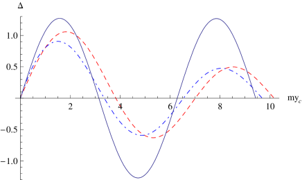
Figure 6: The re-scaled function of $\Delta$ defined by Eq.(6.15), where the dashed, dot-dashed and solid lines are, respectively, for $\Delta\left(x_{0}=0.01\right)/35;\Delta\left(x_{0}=1.0\right)/0.5$ and $\Delta\left(x_{0}=1000\right)/0.005$.

$x_{0}$	$m_{1}y_{c}$	$m_{2}y_{c}$	$m_{3}y_{c}$
0.01	3.82	7.01	10.16
1.0	3.36	6.53	9.69
1000	3.14	6.28	9.42

Table 1: The first three modes $m_{n}\;(n=1,2,3)$ for $x_{0}=0.01,\;1.0,\;1000$, respectively.

Table I shows the first three modes $m_{n}\;(n=1,2,3)$ for $x_{0}=0.01,\;1.0,\;1000$, from which we can see that to find $m_{n}$ it is sufficient to consider only the case where $x_{0}\gg 1$. When $x_{0}\gg 1$ we find that $x_{c}=x_{0}+my_{c}\gg 1$ and AS72

$$J_{1}(x) \simeq \sqrt{\frac{2}{\pi x}}\cos\left(x-\frac{3}{4}\pi\right),$$

$$Y_{1}(x) \simeq \sqrt{\frac{2}{\pi x}}\sin\left(x-\frac{3}{4}\pi\right).$$ (6.16)

Inserting the above expressions into Eq.(6.15), we obtain

$$\Delta = \frac{2}{\pi\sqrt{x_{0}x_{c}}}\sin\left(my_{c}\right),$$ (6.17)

whose roots are given by

$$m_{n}=\frac{n\pi}{y_{c}},\;\;\;(n=1,2,...).$$ (6.18)

In particular, we have

$$m_{1} \simeq 3.14\times\left(\frac{10^{-19}\;{\mbox{m}}}{y_{c}}\right)\;{\mbox{TeV}}$$ (6.19)

$$\simeq \cases{1\;{\mbox{TeV}},&$y_{c}\simeq 10^{-19}\;{\mbox{m}}$,\cr 10^{-2}\;{\mbox{eV}},&$y_{c}\simeq 10^{-5}\;{\mbox{m}}$,\cr 10^{-4}\;{\mbox{eV}},&$y_{c}\simeq 10^{-3}\;{\mbox{m}}$.\cr}$$

It should be noted that the mass $m_{n}$ calculated above is measured by the observer with the metric $\eta_{\mu\nu}$. However, since the warped factor $e^{\sigma(y)}$ is not one at $y=y_{c}$, the physical mass on the visible brane should be given by RS1

$$m^{obs}_{n}=e^{-\sigma\left(y_{c}\right)}m_{n}=\left(\frac{y_{c}+y_{0}}{L}\right)^{1/3}m_{n}.$$ (6.20)

Without introducing any new hierarchy, we expect that $\left[({y_{c}+y_{0})}/{L}\right]^{1/3}\simeq{\cal{O}}(1)$. As a result, we have

$$m^{obs}_{n}=\left(\frac{y_{c}+y_{0}}{L}\right)^{1/5}m_{n}\simeq m_{n}.$$ (6.21)

For each $m_{n}$ that satisfies Eq.(6.15), the wavefunction $\psi_{n}(y)$ is given by

$$\psi_{n}(y) = N_{n}x_{n}^{1/2}\left(\frac{J_{0}\left(x_{n}\right)}{J_{1}\left(x_{0,n}\right)}-\frac{Y_{0}\left(x_{n}\right)}{Y_{1}\left(x_{0,n}\right)}\right),$$ (6.22)

where

$$x_{0,n} \equiv m_{n}y_{0}\simeq n\pi\left(\frac{y_{0}}{y_{c}}\right),$$

$$x_{n} \equiv m_{n}\left(y_{0}+y\right)\simeq n\pi\left(\frac{y_{0}+y}{y_{c}}\right).$$ (6.23)

The normalization factor $N_{n}[\equiv N_{n}\left(m_{n},y_{c}\right)]$ is determined by the condition,

$$\int^{y_{c}}_{0}{\left|\psi_{n}(y)\right|^{2}dy}=1.$$ (6.24)

Figs. 7, 8 and 9 show $\psi_{1}\left(y\right),\;\psi_{2}\left(y\right)$ and $\psi_{3}\left(y\right)$ for $x_{0,1}=100,\;102,\;104$, respectively.

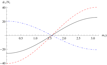
Figure 7: The wavefunction, $\psi_{1}\left(y\right)$, defined by Eq.(6.22) vs $m_{1}y$ where $y\in\left[0,y_{c}\right]$. The dashed, dot-dashed and solid lines are, respectively, for $x_{0,1}=100,\;102,\;104$.

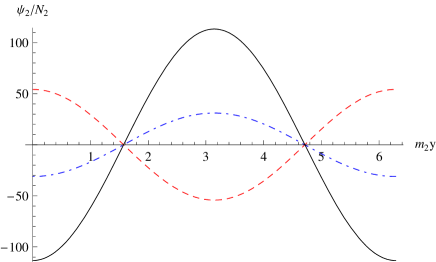
Figure 8: The wavefunction, $\psi_{2}\left(y\right)$, defined by Eq.(6.22), vs $m_{2}y$ where $y\in\left[0,y_{c}\right]$. The dashed, dot-dashed and solid lines are, respectively, for $x_{0,1}=100,\;102,\;104$.

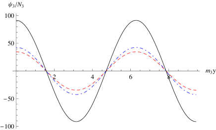
Figure 9: The wavefunction, $\psi_{3}\left(y\right)$, defined by Eq.(6.22), vs $m_{3}y$ where $y\in\left[0,y_{c}\right]$. The dashed, dot-dashed and solid lines are, respectively, for $x_{0,1}=100,\;102,\;104$.

VI.2 4D Newtonian Potential and Yukawa Corrections

To calculate the four-dimensional effective Newtonian potential and its corrections, let us consider two point-like sources of masses $M_{1}$ and $M_{2}$, located on the brane at $y=y_{c}$. Then, the discrete eigenfunction $\psi_{n}(z)$ of mass $m_{n}$ has an Yukawa correction to the four-dimensional gravitational potential between the two particles BS99 ; Csaki00 ,

$$U(r)=G_{4}\frac{M_{1}M_{2}}{r}+\frac{M_{1}M_{2}}{M_{5}^{3}r}\sum_{n=1}^{\infty}{e^{-m_{n}r}\left|\psi_{n}\left(y_{c}\right)\right|^{2}},$$ (6.25)

where $\psi_{n}\left(y_{c}\right)$ is given by Eq.(6.22), with

$$x_{c,n}\equiv m_{n}\left(y_{c}+y_{0}\right)\simeq\frac{n\pi y_{0}}{y_{c}}+n\pi.$$ (6.26)

When $x_{0,1}=m_{1}y_{0}\gg 1$, we find that

$$N_{n} \simeq \frac{\cos\left(2m_{n}y_{0}\right)}{\sqrt{2n\pi y_{0}}},$$

$$\psi_{n}\left(y_{c}\right) \simeq (-1)^{n+1}\sqrt{\frac{2}{y_{c}}}.$$ (6.27)

Then, we obtain,

$$\left|\psi_{n}\left(y_{c}\right)\right|^{2}\simeq 2M_{pl}\left(\frac{l_{pl}}{y_{c}}\right).$$ (6.28)

Clearly, by properly choosing $y_{c}$, the corrections of the 4-dimensional Newtonian potential due to the high order gravitational KK modes are negligible.

VII Conclusions

In this paper, we have systematically studied the possibility of implementing the RS1 scenario RS1 into type II string theory on an $S^{1}/Z_{2}$ orbifold. In particular, in Sec. II, starting with the Neveu-Schwarz/Neveu-Schwarz (NS/NS) sector, we have first compactified the $\left(D+d_{+}+d_{-}\right)$-dimensional spacetime on two manifolds $M_{d_{+}}$ and $M_{d_{-}}$, where the topologies of $M_{d_{+}}$ and $M_{d_{-}}$ are unspecified. As shown explicitly there, this particularly allows the dilaton and modulus fields to have non-zero potentials (masses), which is in contrast to the toroidal compactification considered previously WS07 ; WSVW08 ; WS08 ; TW09 ; LWC00 ; BW06 . After reducing the action to an effective $D$-dimensional one, which is given by Eq.(2.16) in the Einstein frame, we further compactify one of the $(D-1)$ spatial dimensions on an $S^{1}/Z_{2}$ orbifold, by adding the brane actions (2.21). This completes the whole setup of the model to be studied in this paper. Lifting it to the original spacetime, the two orbifold branes become ($D+d_{+}+d_{-}-1$)-dimensional.

In Sec.III, we have explicitly derived the corresponding gravitational and matter field equations both in the bulk and on the branes, by using the Gauss-Codacci and Lanczos equations. In Sec. IV such developed formulas have been applied to cosmology by setting $D=5=d_{+}+d_{-}$. In particular, the generalized Friedmann equations on the branes are given explicitly by Eqs.(4.21) and (4.22).

In Sec. V, in order to study the radion stability and radion mass, we have first derived the general static solutions with a 4-dimensional Poincaré symmetry. Then, using the Goldberger-Wise mechanism, we have studied the radion stability and shown explicitly that it is indeed stable in our current setup. The corresponding radion mass is given by Eq.(5.33), from which we can see that the observational constraint $m_{\varphi}>10^{-3}\;eV$ can be easily satisfied by properly choosing the free parameters presented in the model.

In Sec. VI, we have studied the tensor perturbations, and shown explicitly that the background solution is gravitational stable, and the gravity is localized on the visible brane, as one can be seen clearly from Fig. 5. Due to the particular boundary conditions, the spectrum of the gravitational KK towers is discrete, and the corresponding masses can be well approximated by Eq.(6.18), as one can see from Fig. 6 and Table I. The mass gap $\Delta m\equiv m_{1}$ between the ground state and the first excited state can be in the order of $TeV$, while the high order Yukawa corrections to the 4-dimensional Newtonian potential, due to the high order KK modes, is exponentially suppressed, and can be negligible.

The above results strongly support our earlier conclusions obtained in the studies of orbifold branes in both the HW heterotic M theory GWW07 ; WGW08 and string theory WS07 ; WSVW08 ; WS08 . In particular, in all these models the radion is stable, and the gravity is localized on the visible (TeV) branes, in contrast to the RS1 model RS1 , where the gravity is localized on the invisible brane. Our models are much more complicated than the RS1 model and involve several free parameters. By properly choosing them, the theory should be consistent with observational constraints, a subject that is under our current investigations. It would be also extremely interesting to find specific models in the current setup to explain the late cosmic acceleration of the universe DEs .

References

- (1) V.A. Rubakov, Phys. Usp. 44, 871 (2001); R. Maartens, Living Reviews of Relativity 7 (2004); arXiv:astro-ph/0602415 (2006); P. Brax, C. van de Bruck and A. C. Davis, Rept. Prog. Phys. 67, 2183 (2004); C. Csaki, arXiv:hep-th/0404.096 (2004); V. Sahni, arXiv:astro-ph/0502032 (2005); D. Langlois, arXiv:hep-th/0509231 (2005); R. Durrer, arXiv:hep-th/0507.006 (2005); A. Lue, Phys. Rept. 423, 1 (2006); and D. Wands, arXiv:gr-qc/0601078 (2006).
- (2) H. Horava and E. Witten, Nucl. Phys. B460, 506 (1996); 475, 94 (1996).
- (3) A. Lukas, et al., Phys. Rev. D59, 086001 (1999); Nucl. Phys. B552, 246 (1999).
- (4) J.-L. Lehners, P. Smyth, and K.S. Stelle, Class. Quantum Grav. 22, 2589 (2005).
- (5) Q. Wu, Y.G. Gong, and A. Wang, JCAP, 06, 015 (2009) [arXiv:0810.5377].
- (6) N. Arkani-Hamed, S. Dimopoulos and G. Dvali, Phys. Lett. B429, 263 (1998); Phys. Rev. D59, 086004 (1999); and I. Antoniadis, et al., Phys. Lett., B436, 257 (1998).
- (7) L. Randall and R. Sundrum, Phys. Rev. Lett. 83, 3370 (1999).
- (8) J. Cline, C. Grojean, and G. Servant, Phys. Rev. Lett. 83, 4245 (1999); C. Csaki et al, Phys. Lett. B462, 34 (1999).
- (9) H. Davoudiasl, J.H. Hewett, and T.G. Rizzo, Phys. Rev. Lett. 84, 2080 (2000); G.F. Giudice, R. Rattazzi, and J.D. Wells, Nucl. Phys. B595, 250 (2001); G.D. Krib, “Physics of the radion in the Randall-Sundrum scenario,” arXiv:hep-th/0110242; H. Davoudiasl, J.H. Hewett, and T.G. Rizzo, Phys. Rev. D63, 075004 (2001); T.G. Rizzo, JHEP, 06, 056 (2002); D. Dominici et al, Nucl. Phys. B671, 243 (2003); J.F. Gunion, M. Toharia, and J.D. Wells, Phys. Lett. B585, 295 (2004); M. Carena et al, Phys. Rev. D76, 035006 (2007); L. Fitzpatrick et al, “Searching for the Kaluza-Klein Gravity in Bulk RS Models,” arXiv:hep-ph/0701150; C. Csaki, J. Hubisz, and S.J. Lee, “radion Phenomenology in Realistic Warped Space Models,” arXiv:0705.3844; H. Davoudiasl, T.G. Rizzo, and A. Soni, “On Direct Verification of Warped Hierarchy-and-Flavor Models,” arXiv:0710.2078; O. Antipin and A. Soni, “Towards establishing the spin of warped gravitons,” arXiv:0806.3427; L. Randall and M.B. Wise, arXiv:0807.1746; and references therein.
- (10) S. Weinberg, Rev. Mod. Phys. 61, 1 (1989); S.M. Carroll, arXiv:astro-ph/0004075; T. Padmanabhan, Phys. Rept. 380, 235 (2003); S. Nobbenhuis, arXiv:gr-qc/0411093; J. Polchinski, arXiv:hep-th/0603249; and J.M. Cline, arXiv:hep-th/0612129.
- (11) C. Csaki, J. Erlich, and C. Grojean, Gen. Relativ. Grav. 33, 1921 (2001).
- (12) N. Arkani-Hamed, et al, Phys. Lett. B480, 193 (2000); and S. Kachru, M.B. Schulz, and E. Silverstein, Phys. Rev. D62, 045021 (2000).
- (13) Y. Aghababaie, et al, Nucl. Phys. B680, 389 (2004); JHEP, 0309, 037 (2003); C.P. Burgess, Ann. Phys. 313, 283 (2004); AIP Conf. Proc. 743, 417 (2005); and C.P. Burgess , J. Matias, and F. Quevedo, Nucl.Phys. B706, 71 (2005).
- (14) S. Forste, et al, Phys. Lett. B481, 360 (2000); JHEP, 0009, 034 (2000); C. Csaki, et al, Nucl. Phys. B604, 312 (2001); and J.M. Cline and H. Firouzjahi, Phys. Rev. D65, 043501 (2002).
- (15) K. Koyama, arXiv:0706.1557; and C.P. Burgess, arXiv:0708.0911.
- (16) G. R. Dvali, G. Gabadadze and M. Porrati, Phys. Lett. B484, 112 (2000).
- (17) L. Randall and R. Sundrum, Phys. Rev. Lett. 83, 4690 (1999).
- (18) C. Deffayet, Phys. Lett. B502, 199 (2001); V. Sahni and Yu. Shtanov, JCAP, 11, 014 (2003); A. Lue, Phys. Report, 423, 1 92006); R. Maartens, arXiv;astro-ph/0602415 (2006); and references therein.
- (19) M.A. Luty, M. Porrati, and R. Rattazzi, JHEP, 0309, 029 (2003); A. Nicolis, and R. Rattazzi, ibid., 0406, 059 (2004); K. Koyama, Physics. Rev. D72, 123511 (2005); K. Koyama and S. Sibiryakov, ibid., 73, 044016 (2006); C. Charmousis, R. Gregory, N. Kaloper, and A. Padilla, JHEP, 0610, 066 (2006); R. Gregory, N. Kaloper, R.C. Myers, and A. Padilla, “A New perspective on DGP Gravity,” arXiv:0707.2666; K. Koyama, “Ghosts in the self-accelerating universe,” arXiv:0709.2399.
- (20) C. Deffayet, G. Gabadadze, and A. Iglesias, JCAP, 0608, 012 (2006); D. Dvali, New J. Phys. 8, 326 (2006).
- (21) W. Fang, et al., “Challenges to the DGP Model from Horizon-Scale Growth and Geometry,” Phys. Rev. D, in press (2009) [arXiv:0808.2208].
- (22) Y. Gong, M. Ishak, and A. Wang, “Growth factor parametrization in curved space,” arXiv:0903.0001.
- (23) K. Benakli, Int. J. Mod. Phys. D8, 153 (1999); H.S. Reall, Phys. Rev. D59, 103506 (1999); A. Lukas, B.A. Ovrut, and D. Waldram, ibid., 60, 086001 (1999).
- (24) W. Chen, et al, Nucl. Phys. B732, 118 (2006); J.-L. Lehners, P. McFadden, and N. Turok, Phys. Rev. D75, 103510 (2007).
- (25) Y.-G. Gong, A. Wang, and Q. Wu, Phys. Lett. B663, 147 (2008) [arXiv:0711.1597].
- (26) A. Wang and N.O. Santos, Phys. Lett. B669, 127 (2008) [arXiv:0712.3938].
- (27) Q. Wu, N.O. Santos, P. Vo, and A. Wang , JCAP 09, 004 (2008) [arXiv:0804.0620].
- (28) A. Wang and N.O. Santos, arXiv:0808.2055.
- (29) W. Fischler, et al., JHEP, 07, 003 (2001); J.M. Cline, ibid., 08, 035 (2001); E. Halyo, ibid., 10, 025 (2001); S. Hellerman, ibid., 06, 003 (2003).
- (30) L.M. Krauss and R.J. Scherrer, Gen. Relativ. Grav. 39, 1545 (2007); and references therein.
- (31) J.E. Lidsey, D. Wands, and E.J. Copeland, Phys. Rept. 337, 343 (2000).
- (32) T. Battefeld and S. Watson, Rev. Mod. Phys. 78, 435 (2006).
- (33) A. Tziolas, A. Wang, and Z.C. Wu, JHEP, in press (2009) [arXiv:0812.1377]; and P. Sharma, A. Tziolas, and A. Wang, arXiv:0901.2676.
- (34) P.K. Townsend and N.R. Wohlfarth, Phys. Rev. Lett. 91, 061302 (2003).
- (35) G. W.Gibbons in Supersymmetry, Supergravity and Related Topics, edited by F. de Aguila, et al (Sigapore, World Scientific, 1985), p.124; J.M. Maldacena and C. Nuñez, Int. J. Mod. Phys. A16, 822 (2001).
- (36) N. Ohta, Phys. Rev. Lett. 91, 061303 (2003).
- (37) N.R. Wohlfarth, Phys. Lett. B563, 1 (2003); S. Roy ibid., 567, 322 (2003).
- (38) J.K. Webb, et al, Phys. Rev. Lett. 87, 091301 (2001); J.M. Cline and J. Vinet, Phys. Rev. D68, 025015 (2003); N. Ohta, Prog. Theor. Phys. 110, 269 (2003); Int. J. Mod. Phys. A20, 1 (2005); C.M. Chen, et al, JHEP, 10, 058 (2003); E. Bergshoeff, Class. Quantum Grav. 21, 1947 (2004); Y. Gong and A. Wang, ibid., 23, 3419 (2006); I.P. Neupane and D.L. Wiltshire, Phys. Rev. D72, 083509 (2005); Phys. Lett. B619, 201 (2005); K. Maeda and N. Ohta, ibid., B597, 400 (2004); Phys. Rev. D71, 063520 (2005); K. Akune, K. Maeda and N. Ohta, ibid., 103506 (2006) V. Baukh and A. Zhuk, ibid., 73, 104016 (2006); A. Krause, Phys. Rev. Lett. 98, 241601 (2007); I.P. Neupane, ibid., 98, 061301 (2007); and references therein.
- (39) M. Gasperini, Elements of String Cosmology (Cambridge University Press, Cambridge, 2007).
- (40) F. Leblond, R.C. Myers, and D.J. Winters, JHEP, 07, 031 (2001).
- (41) P. Binétruy, C. Deffayet, U. Ellwanger, and D. Langlois, Phys. Lett. B477, 285 (2000); and P. Binétruy, C. Deffayet, and D. Langlois, Nucl. Phys. B615, 219 (2001).
- (42) A. Wang, R.-G. Cai, and N.O. Santos, Nucl. Phys. B797, 395 (2008) [arXiv:astro-ph/0607371].
- (43) T. Shiromizu, K.-I. Maeda, and M. Sasaki, Phys. Rev. D62, 024012 (2000); A.N. Aliev and A.E. Gumrukcuoglu, Class. Quantum Grav. 21, 5081 (2004); and R.-G. Cai and L.-M. Cao, Nucl. Phys. B785, 135 (2007).
- (44) C. Lanczos, Phys. Z. 23, 539 (1922); and Ann. Phys. (Germany), 74, 518 (1924).
- (45) J. Martin, G.N. Felder, A.V. Frolov, M. Peloso, and L.A. Kofman, Phys. Rev. D69, 084017 (2004).
- (46) W.D. Goldberger and M.B. Wise, Phys. Rev. Lett. 83, 4922 (1999); and Phys. Lett. B475, 275 (2000).
- (47) M. Abramowitz and I.A. Stegun, Handbook of Mathematical Functions (Dover Publications, INC., New York, 1972), pp.374-8.
- (48) J. Garriga and T. Tanaka, Phys. Rev. Lett. 84, 2778 (2000); T. Tanaka and X. Montes, Nucl. Phys. B582, 259 (2000).
- (49) C. Csaki, J. Erlich, T. J. Hollowwood, and Y. Shirman, Nucl. Phys. B581, 309 (2000).
- (50) C. Csaki, M.L. Graesser, and G.D. Kribs, Phys. Rev. D63, 065002 (2001).
- (51) C. Cohen-Tannoudji, B. Diu, and F. Laloë, Quantum Mechanics, Vols. I II (John Wiley Sons, New York, 1977).
- (52) A. Brandhuber and K. Sfetsos, JHEP, 10, 013 (1999).
- (53) V. Sahni and A. A. Starobinsky, Int. J. Mod. Phys. D 9, 373 (2000); P.J.E. Peebles and B. Ratra, Rev. Mod. Phys 75, 559 (2003); T. Padmanabhan, Phys. Rep. 380, 235 (2003); V. Sahni, arXiv:astro-ph/0403324 (2004); E.J. Copeland, M. Sami, and S. Tsujikawa, Int. J. Mod. Phys. D15, 1753 (2006); E. Linder, arXiv:0801.296; and J.A. Frieman, M.S. Turner, and D. Huterer, arXiv:0803.0982.