Off-diagonal geometric phase of atom-electron coupling in hydrogen atom

Abstract

In this paper, the off-diagonal geometric phase of thermal state in hydrogen atom under the effects of external magnetic field is considered. Increasing temperature tends to suppress the off-diagonal geometric phase, including $1$-order and $2$-order cases. On the other hand, the relationship between the geometric phase and external magnetic field is discussed.

1 Introduction

The concept of geometric phase (GP) was first introduced by Panchartnam in his study of interference of classical light in distinct states of polarization [1]. Berry’s work showed a quantum pure state can retain the information of its motion when it undergoes a cyclic evolution [2]. Simon [3] subsequently recasted the mathematical formation of Berry phase with the language of differential geometry and fibre bundles. He observed that the origin of Berry phase is attributed to the holonomy in the parameter space. Due to its robustness to imperfections, such as docoherence and the random unitary perturbations, geometric phase has many applications in the field of quantum information processing and condensed matter physics. It has been pointed out that the non-Abelian holonomy may be used in the construction of universal sets of quantum gates for the purpose of achieving fault-tolerant quantum computation [4, 5]. On the other hand, GP, being a measure of the curvature of the Hilbert space, when associated with the energy crossing has a peculiar behavior near the degeneracy point. GP may be considered as a good candidate for a universal order parameter for quantum phase transitions [6, 7].

In the early discussions, most researches were focused on the evolution of pure states. In realistic world, due to the effect of environment, the most states are mixed. Uhlmann was probably the first to address the issue of mixed state holonomy, but as a purely mathematical problem [8, 9]. Later Sjöqvist et al. discussed the geometric phase for non-degenerate mixed state under unitary evolution in Ref.[10], basing on the Mach-Zender interferometer. Singh et al.[11] gave a kinematic description of the mixed-state GP in Ref.[10] and extended it to degenerate density operators. The generalization to nonunitary evolution has also been adressed in Refs.[12].

Later it was found that the above diagonal GP itself could not exhaust al information contained in phases acquired when the quantal system undergoes an adiabatic evolution. The notions of GP break down in cases where the inteference visibility between the initial and final states vanishes. This gives rise to the definition of the off-diagonal geometric phase factor [13]. Here, The concept of Berry phase was extended to the the evolution of more than one state. They found a set of independent off-diagonal phase factors that exhaust the geometrical phase information carried by the basis of eigenstates along the path. Later, the concept of off-diagonal GP was extended to the cases of mixed states[14].

The off-diagonal geometric phase factor of the degenerate mixed states was defined as [15]

$$\gamma^{(l)}=\Phi\left[Tr(\sum_{\alpha=1}^{l}U(\tau)V_{j_{\alpha}}^{\parallel}(\tau)\sqrt[l]{\rho_{j_{\alpha}}})\right]$$ (1)

where $\Phi[z]\equiv z/|z|$ for any nonzero complex number $z$. The phase is manifestly gauge invariant. $U(\tau)$ is the unitary evolution operator and $U(\tau)=\exp(-i\tau H/\hbar)$ and $H$ is the total Hamiltonian. Throughout this paper, Planck’s constant $\hbar$ is set to unity for simplicity. One can define a set of noninterfering density operators,

$$\rho_{n}=\lambda_{1}P_{n;1}^{(m_{1})}+\cdots\lambda_{K}P_{n;K}^{(m_{K})},n=1,\ldots,N,$$ (2)

where $P_{n;k}^{(m_{k})}=W^{n-1}P_{1;k}^{(m_{k})}(W^{\dagger})^{n-1}$ and $W$ is a permutation unitarity as $W=|\psi_{1}\rangle\langle\psi_{N}|+|\psi_{N}\rangle\langle\psi_{N-1}|+\cdots|\psi_{2}\rangle\langle\psi_{1}|$.

The parallel transport unitary operator for $\rho_{n}$ may be expressed as $U_{n}^{\parallel}(t)=U(t)V_{n}^{\parallel}(t)$ with supplementary operators $V_{n}^{\parallel}(t)=\alpha_{n;1}^{\parallel}(t)+\dots+\alpha_{n;k}^{\parallel}(t)$, where

$$\alpha_{n;k}^{\parallel}=P_{n;k}^{m_{k}}\mathbf{T}\exp\left(-\int_{0}^{t}P_{n;k}^{m_{k}}U^{\dagger}(t^{\prime})\dot{U}(t^{\prime})P_{n;k}^{m_{k}}dt^{\prime}\right)P_{n;k}^{m_{k}}.$$ (3)

$\mathbf{T}$ denotes time ordering. $P_{n;k}^{m_{k}}$ is the projector of rank $m_{k}$ onto the $m_{k}$-fold degenerate eigenspace.

When the Hamiltonian is independent of the time $t$, $\alpha_{n;k}^{\parallel}$ will be reduced as follows,

$$\alpha_{n;k}^{\parallel}=P_{n;k}^{m_{k}}\mathrm{T}\exp(itP_{n;k}^{m_{k}}HP_{n;k}^{m_{k}})P_{n;k}^{m_{k}}.$$ (4)

Apparently $\gamma^{(1)}$ are the standard mixed-state geometric phase factors associated with the unitary paths in state space. The off-diagonal mixed-state geometric phases contain information about the geometry of state space along the path connecting pairs of density operators, when the standard mixed-state geometric phases are undefined. The uncontained information can be shown via high-order off-diagonal geometric phase. The $l=2$ case has been discussed in terms of two-particle interferometry [16].

The off-diagonal geometric phase for some models has been discussed. For example, X.X. Yi et al.[17] investigated the effect of the intersubsystem coupling on the off-diagonal geometric phase in a composite system, where the system undergoes an adiabatic evolution.

2 Model

In this paper, the thermal state of the hydrogen atom is discussed. As one knows, in the hydrogen atom, the electron spin is coupled to the nuclear spin by the hyperfine interaction. The hyperfine line for the hydrogen atom has a measured magnitude of 1420 MHz in frequency. Some calculation on the basis of first-order perturbation for the magnetic dipole interaction between the electron and nucleus gives contribution to the coupling strength of $\mathbf{I}\cdot\mathbf{S}$ term. Taking account of the effect of an external magnetic field, one can have a model Hamiltonian which is [18]

$$H_{0}=J(I_{x}\otimes S_{x}+I_{y}\otimes S_{y}+I_{z}\otimes S_{z})$$ (5)

where $J$ is the coupling constant. Here the electronic orbital angular momentum $L$ is assumed to be zero.

As we know, for a hydrogen atom, the nucleus and electron has both spin-1/2, $\mathbf{I}=\mathbf{S}=\frac{1}{2}\mathbf{\sigma}$. The Hamiltonian Eq.5 has $2$ district eigen-energies: $1/4J$ and $-3J/4$ and the former is 3-fold degenerate with eigenvestors: $|\phi_{i}\rangle,i=1,2,3$ and the latter is non-degenerate with eigenvector $|\phi_{4}\rangle$. The four eigenvectors are given by

$$|\phi_{1}\rangle = |00\rangle$$

$$|\phi_{2}\rangle = \frac{1}{\sqrt{2}}(|01\rangle+|10\rangle)$$

$$|\phi_{3}\rangle = |11\rangle$$

$$|\phi_{4}\rangle = \frac{1}{\sqrt{2}}(|01\rangle-|10\rangle)$$

Now the atom is assumed to be under the temperature $T$. Due to the effect of the temperature, the state of the atom is highly mixed. The density matrix can be written in terms of partition function $\rho=e^{-\beta H}/tre^{-\beta H},$ where $\beta=1/kT$ and $k$ is Boltzmann’s constant and it is set to unity throughout this paper. $T$ denotes the temperature. Due to the effect of thermal fluctuation, the system is highly mixed. At the initial time $t=0$, no magnetic field is imposed so the density matrix of the initial state is given by

$$\rho_{0}=\frac{e^{-\beta H_{0}}}{tre^{-\beta H_{0}}}.$$ (6)

One can see the above $4$ eigenvectors are also the eigenvectors of $\rho_{0}$. After the initial time $t=0$, the external magnetic field is imposed upon the system and the Hamiltonian will be $H=H_{0}+H_{I}$. The degeneracy of the state is destroyed due to the magnetic field. The interaction term $H_{I}$ is given by

$$H_{I}=CI\otimes S_{z}+DI_{z}\otimes I.$$ (7)

The parameters $C$ and $D$ are related with external magnetic fields,

$$C=g\mu_{B}B,\ \ D=-\frac{\mu}{I}B.$$

The nuclear magnetic moment $\mu$ equals $2.793\mu_{N}$ where $\mu_{N}=e\hbar/(2m_{p})$. In general C is much larger than D, $|C/D|\sim m_{p}/m_{e}\approx 2000$, so for most applications D may be neglected. At the same level of approximation the $g$ factor of the electron may be put equal to 2. Therefore one has

$$H_{I}=g\mu_{B}BI\otimes S_{z}.$$

It is obvious that the commutation $[H_{0},H_{I}]\neq 0$. It implies that the external magnetic field will drive the system to involve with the time. At time $t$, the state is

$$\rho(t)=U(t)\rho_{0}U^{\dagger}(t)$$

where the unitary matrix $U(t)=\exp\{-iHt\}$. Assuming after a period $T$, the state evolves to its initial state $\rho(0)$, i.e., $\rho(0)=\rho(T)$, then one has

$$T=\frac{2n\pi}{\sqrt{C^{2}+J^{2}}}.$$ (8)

Here we restrict ourselves to $n=1$. Here $C=g\mu_{B}B$ which is the function of magnetic field $B$, so one can see the magnetic field $B$ and coupling constant $J$ can control the period $T$. After a period evolution, a mixed-state geometric phase can be observed. In next section, we will discuss this mixed-state geometric phase.

3 Geometric Phase

It is obvious that the initial mixed state $\rho_{0}=e^{-\beta H}/tre^{-\beta H}$ is degenerate. In Ref.[19], A.T. Rezakhani and P. Zanardi studied the GP of an open quantum system interaction with a thermal environment by using the definition given in Ref.[15]. In sect.1, the shortcoming of the definition has been discussed. To overcome the shortcoming, we will use the definition of off-diagonal GP given by Eq.1 to evaluate the GP of the state to study the information which are not exhausted by diagonal GP.

3.1 1-order GP

The $1$-order off-diagonal GP is equivalent to the ordinary diagonal GP which is thought not to exhaust the information about the geometry of state along the path connecting pairs of density operators.

The initial density matrix $\rho_{1}$ can be written as $\rho_{1}=\sum_{i=1}^{3}\lambda_{1}|\phi_{i}\rangle\langle\phi_{i}|+\lambda_{2}|\phi_{4}\rangle\langle\phi_{4}|.$ There are two eigenspaces. The first space is $3$-Dimensional and the second one is $1$-dimensional. From Eq.1, the $1$-order off-diagonal GP can be reduced to

$$\gamma^{(1)}=\Phi\left(trU(\tau)V_{1}^{\parallel}\rho_{1}\right),$$ (9)

where $U(\tau)$ is the unitary operator. $V_{1}^{\parallel}=\alpha_{1;1}^{\parallel}(t)+\alpha_{1;2}^{\parallel}(t)$ which are the unitary on the first and second degenerate subspaces.

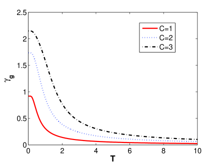
Figure 1: First order off-diagonal GP $\gamma_{g}$ versus temperature $T$, when $C=g\mu_{B}B$ are 1,2,3 respectively.

Fig.1 shows the effect of temperature upon GP, one can see increasing temperature tends to suppress GP. Fig.2 shows the relation between GP and the external magnetic field $B=C/g\mu_{B}$. One can see when $B$ changes its direction, GP is not changed. When increasing of the length of magnetic field tends to enhance GP. So that one can control GP via manipulating the magnetic field. From the figure, one can see that for a relatively large temperature interval geometric phase is varying very slowly with temperature. When $C=0$, the geometric phase vanishes. It is trivial because in this case no magnetic field is imposed so that the state will not evolve with the time. When the temperature approaches infinity, i.e., $\beta$ approaches zero, the matrix $e^{-\beta H}$ will become an identity matrix, so that the unitary matrix $U(t)$ will be commutative with the initial state and the state will not evolve with the time. There is no GP can be detected.

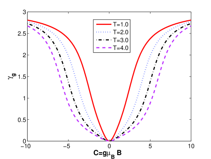
Figure 2: First order off-diagonal GP $\gamma_{g}$ versus external magnetic field $C=g\mu_{B}B$, when the temperature $T=1.0,2.0,3.0,4.0$ respectively.

3.2 2-order GP

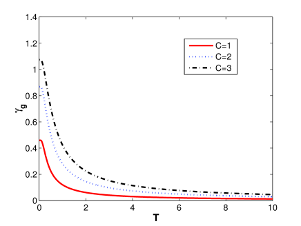
Figure 3: Second order off-diagonal GP$\gamma_{g}$ versus temperature $T$, when $C=g\mu_{B}B$ are 1,2,3 respectively.

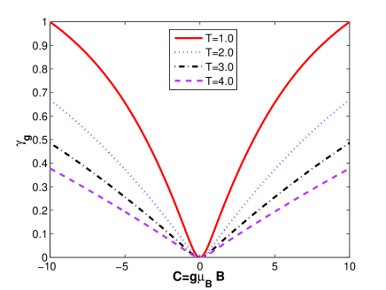
Figure 4: Second order off-diagonal GP $\gamma_{g}$ versus external magnetic field $C=g\mu_{B}B$, when the temperature $T=1.0,2.0,3.0,4.0$ respectively.

Fig.3 shows the relationship between 2-order off-diagonal GP and the temperature. The $2$-order off-diagonal GP can show other information which the diagonal GP cannot exhaust. Also one can see increasing temperature tends to suppress the 2-order off-diagonal GP.

One can test the existence of off-diagonal geometric phase of the above model. If one would detect such a phase the system should be at low temperature, due to rapid decay of geometric phase with temperature.

One can evaluate the mixedness of the state. The mixedness is defined as $V=1-tr\rho(t)^{2}$. According to $\rho(t)=e^{-iHt}\rho_{0}e^{iHt}$, one can easily obtain the mixedness of the state $\rho(t)$ as

$$V=1-tr\rho(t)^{2}=1-tr\left[U(t)\rho_{0}U^{\dagger}(t)U(t)\rho_{0}U^{\dagger}(t)\right]=\frac{6(1+e^{\frac{J}{kT}})}{(3+e^{\frac{J}{kT}})^{2}}.$$ (10)

From Eq.10, one can see when the temperature increasing, the mixedness is increased. When the temperature approaches infinity, the mixedness approaches $3/4$. Note the mixedness is not varied with the time, but it is the function of temperature. With the increasing temperature of environment, the thermal fluctuation of the system is enhanced and the coupling of the system and environment thermal bath is also enhanced. The enhanced thermal fluctuations suppress the GP of the system.

4 Summary

We have demonstrated the effect of temperature upon the off-diagonal geometric phase. It shows that increasing temperature tends to suppress the off-diagonal GP. Comparing ordinary diagonal GP, off-diagonal GP can reveal more information which is not exhausted by standard diagonal GP. As the temperature is increased, the thermal fluctuation will dominate the behavior of the particles and it will suppress the GP.

The work was supported by CJLU Grant No. 01101-000174.

References

- [1] S. Pacharatnam, Proc. Indian. Acad. Sci. Set. A, 44, 247 (1956).
- [2] M. V. Berry, Proc. R. Soc. London A. 392, 45 (1984).
- [3] B. Simon, Phys. Rev. Lett. 51, 2167 (1983)
- [4] P. Zanardi and M. Rasetti Phys. Lett. A, 264, 94 (1999).
- [5] J. Pachos, P. Zanardi, and M. Rasetti, Phys. Rev. A 61, 010305(R) (2000)
- [6] A.C.M. Carollo and J.K. Pachos, Phys. Rev. Lett. 95, 157203 (2005).
- [7] S.-L. Zhu, Phys. Rev. Lett. 96, 077206 (2006).
- [8] A. Uhlmann, Rep. Math. Phys. 24, 229 (1986).
- [9] A. Uhlmann, Lett.Math. Phys. 21, 229 (1991).
- [10] E. Sjöqvist, A. K. Pati, A. Ekert, J. S. Anandan, M. Ericsson, D. K. L. Oi, V. Vedral, Phys. Rev. Lett. 85, 2845 (2000).
- [11] K. Singh, D.M. Tong, K. Basu, J.L. Chen, and J.F. Du, Phys. Rev. A 67, 032106 (2003).
- [12] D. M. Tong, E. Sjöqvist, L. C. Kwek, C. H. Oh, Phys. Rev. Lett. 93, 080405 (2004).
- [13] N. Manini and F. Pistolesi, Phys. Rev. Lett. 85, 3067 (2000).
- [14] S. Filipp and E. Sjöqvist, Phys. Rev. Lett. 90, 050403 (2003).
- [15] D.M. Tong, E. Sjöqvist, S. Filipp, L.C. Kwek and C.H. Oh, Phys,. Rev. A 71, 032106 (2005).
- [16] S. Filipp and E. Sjöqvist, Phys. Rev. A 65, 052111 (2003); S. Filipp and E. Sjöqvist, Phys. Rev. A 68, 042112 (2003).
- [17] X.X. Yi and J.L. Chang, Phys. Rev. A 70, 012108 (2004).
- [18] C. J. Pethick, H. Smith, Bose-Einstein Condensation in Dilute Gases, Cambridge Press, Cambridge, 2002.
- [19] A.T. Rezakhani and P. Zanardi, Phys. Rev. A 73, 052117 (2006).