The ion-induced charge-exchange X-ray emission of the Jovian Auroras: Magnetospheric or solar wind origin?

Abstract

A new and more comprehensive model of charge-exchange induced X-ray emission, due to ions precipitating into the Jovian atmosphere near the poles, has been used to analyze spectral observations made by the Chandra X-ray Observatory. The model includes for the first time carbon ions, in addition to the oxygen and sulfur ions previously considered, in order to account for possible ion origins from both the solar wind and the Jovian magnetosphere. By comparing the model spectra with newly reprocessed Chandra observations, we conclude that carbon ion emission provides a negligible contribution, suggesting that solar wind ions are not responsible for the observed polar X-rays. In addition, results of the model fits to observations support the previously estimated seeding kinetic energies of the precipitating ions ($\sim$0.7-2 MeV/u), but infer a different relative sulfur to oxygen abundance ratio for these Chandra observations.

1 Introduction

Since the first generation of X-ray observatories, Jupiter has been one of the primary solar system objects of interest. In fact, Jovian X-ray emission was first detected by the Einstein observatory (Metzger et al., 1983), then studied with ROSAT (Waite et al., 1994; Gladstone et al., 1998), and two distinct components were identified, namely emission from the high-latitude (polar) and low-latitude (equatorial) regions. Various explanations of the origin of these emissions were put forth but could not be stringently tested due to the poor spatial and spectral (${\cal E}/\Delta{\cal E}<1$) resolution of the early measurements. However, recent observations with Chandra and XMM-Newton have provided unprecedented resolution on the planet (Gladstone et al., 2002; Elsner et al., 2005; Branduardi-Raymont et al., 2004, 2007a, 2007b, 2008; Bhardwaj et al., 2005, 2006) and thorough analysis of the observational data have confirmed and refined the characteristic difference between Jovian polar and disk emission. It is now generally accepted that the disk component is due to the scattering and fluorescence of solar X-rays in the atmosphere (Maurellis et al., 2000; Branduardi-Raymont et al., 2007b; Bhardwaj et al., 2005, 2006; Cravens et al., 2006). In contrast, a mounting body of evidence favors the charge-exchange (CX) model as the basic explanation of the Jovian X-ray polar auroras. This model assumes highly energetic heavy ions precipitating into the Jovian atmosphere and emitting K- and L-shell photons after cascading from their excited states (Metzger et al., 1983; Horanyi et al., 1988; Waite et al., 1994; Cravens et al., 1995; Kharchenko et al., 1998; Liu & Schultz, 1999; Kharchenko et al., 2006, 2008).

However, fundamental questions remain unanswered, such as What is the detailed mechanism of ion acceleration before emission; What is the source of the heavy ions (do they originate from the Jovian magnetosphere and are therefore closely coupled with its ion-rich satellites, or are they of solar wind origin); and What are the composition of the ion fluxes and their initial kinetic energies at the top of the Jovian atmosphere (Cravens et al., 2003)? Observations and interpretive models answering these questions would advance our knowledge of the Jovian system and, by extension, of other planetary atmospheres and environments. Toward these ends, many studies have been carried out seeking to explain the observed spectral features by fitting them with a continuum plus ion emission lines (e.g., Elsner et al., 2005; Branduardi-Raymont et al., 2004, 2007a, 2007b). In order to reflect the intrinsic correlations between the intensities of different X-ray lines induced by individual ions, CX models were developed to produce synthetic spectra. These spectra could, in turn, be used to infer parameters such as relative ion abundances and initial energies required to account for the observations. Early CX models were restricted to oxygen ion precipitation (Cravens et al., 1995; Kharchenko et al., 1998; Liu & Schultz, 1999) owing to the lack of extensive atomic data required by the models (i.e., energy-dependent, state-selective charge exchange cross sections for all ionization stages of the ions and transition probabilities for radiative and non-radiative de-excitation, etc.).

Since oxygen ions contributing to the Jovian X-ray auroras could originate either in the vicinity of Jupiter or from the solar wind, the next level of discrimination between these two possible sources was provided by including sulfur ions because of their great magnetospheric abundance. This was enabled by the advent of large scale atomic collision and structure calculations, and recently included in the CX model (Kharchenko et al., 2006, 2008). These results provided an improved fit to the observations and gave indications of the range of initial energies of the ions at the top of Jupiter’s atmosphere. Here, we seek to further constrain the origin and characteristics of the X-ray emission through (i) the addition of carbon to the model, again enabled by newly available atomic data, (ii) significantly increasing the level of detail of the treatment of radiative transitions, and (iii) using a more sophisticated methodology to fit the synthetic spectra to observations through systematic variation of the input ion abundances and kinetic energies.

In this Letter, we report the results of this more complete CX model of the Jovian auroral X-ray emission. The basic structure and major improvements of the model are described in Section 2. In Section 3 a description is given of how our results have been fit to Chandra observations with the X-ray spectral fitting software Xspec (Arnaud, 1996). Finally, discussion and interpretation of the X-ray emission modeling results are given in Section 4.

2 Ion-induced charge-exchange emission model

A description of the basic CX model along with its development has been given previously by Kharchenko et al. (1998), Liu & Schultz (1999), Kharchenko & Dalgarno (2000), and Kharchenko et al. (2006, 2008), and in various reviews (e.g., Bhardwaj & Gladstone, 2000; Bhardwaj et al., 2007). In brief, we begin with the Monte Carlo (MC) simulation developed by Kharchenko et al. (2008) to treat the ion precipitation and CX collisions during the ion’s deceleration through the atmosphere. Modeling the energy loss and capture into the excited states that seed subsequent radiative emission involves three collision channels – charge exchange, target ionization, and electron stripping from the ions. Each channel has an associated energy loss contributing to the stopping process, and stripping and charge exchange change the ion’s charge state. CX leads to population of excited states that result in photon emission or, less frequently, decay non-radiatively. A synthetic spectrum is built up by tracing all possible cascading paths after these excited states are populated.

Specifically, we set the total number of ions, $N_{\rm tot}$, to 1000 in the MC simulation for each species considered; increasing this number makes negligible changes to the final synthetic spectrum. As pointed out by Kharchenko et al. (2008), the spectra are not sensitive to the initial charge states of the ions for a fixed ion energy at the top of Jupiter’s atmosphere, so we choose singly charged ions (e.g., O⁺) to begin the precipitation process. The energy loss of the ions due to collisions in all three channels are as formulated by Kharchenko et al. (1998). A simulation terminates when the ion slows down to the point that further X-ray emission is negligible.

The most significant improvement in the present work is the incorporation of carbon ions as a new source of X-ray emission, in addition to the previously considered oxygen and sulfur, in order to introduce an abundant, more distinctly solar wind originating species. This is motivated by Chandra and XMM-Newton observations (Gladstone et al., 2002; Branduardi-Raymont et al., 2008) which appear to overturn the early hypothesis that the auroral X-ray emission was linked to ions flowing along magnetic field lines from the Io plasma torus. These new observations indicated that the X-ray emission comes from latitudes higher than those which are magnetically connected to flux from the orbital radius of Io. Thus, other sources have been suggested including from more distant regions of the magnetosphere and the solar wind (e.g., Mauk et al., 2003; Cravens et al., 2003).

The MC simulation tracks the energy loss and charge state change at each collision according to the probabilities established by the relevant atomic cross sections (Schultz et al., 2009) and, for each CX collision, records the charge state and ion energy. At the end of the simulation the CX number distribution, $N^{\rm CX}(q,E)$, is tabulated, where $q$ and $E$ are the charge state and the energy, respectively. The calculated probabilities for state-selective capture (Schultz et al., 2009) are then multiplied by $N^{\rm CX}(q,E)$ to obtain the initial population $X(q,E;\gamma)$ where $\gamma$ represents the energy level ($n,\ell$) of each ion populated by a CX collision.

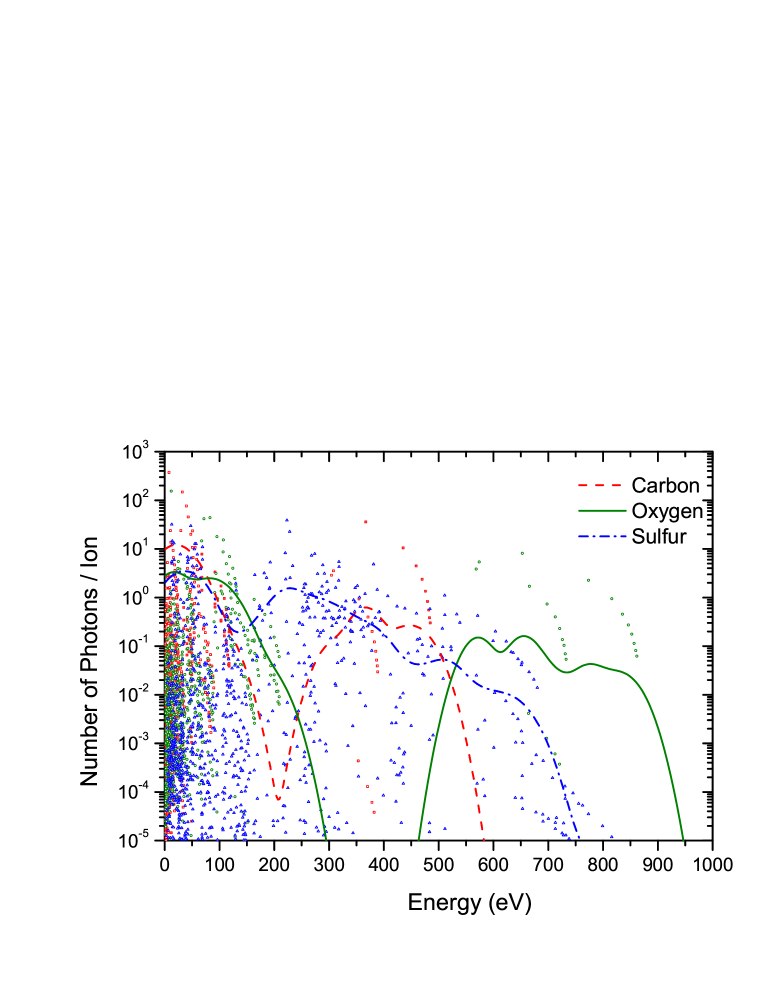
The next step in producing a synthetic spectrum is to calculate the radiative transition matrices, $T(q;\gamma^{\prime},\gamma)$, which describes the pathway from any initial state ($\gamma$) to any final state ($\gamma^{\prime}$), as described by Kharchenko et al. (1998) and Kharchenko & Dalgarno (2000). For the present work, we collected atomic transition data from the Atomic Spectra Database (Ralchenko et al., 2008), the Atomic Line List (van Hoof, 1999), and recent results for several ion species (Johnson et al., 2002; Kingston et al., 2002; Nahar, 2002). In total, we include 960 carbon, 954 oxygen, and 1512 sulfur emission lines when calculating the transition matrices (but in the subsequent model fit to the X-ray spectra we only consider lines with photon energy above 200 eV). This is an elaboration of the model beyond our earlier work (Kharchenko et al., 2008) which used energy-independent photon yield tables and chose only the most prominent lines of oxygen (12 lines) and sulfur (27 lines). Given the transition matrices, the photon yields from the cascade process are determined by $Y(q,E;\gamma^{\prime},\gamma)=T(q;\gamma^{\prime},\gamma)\times X(q,E;\gamma)$ and the synthetic spectrum is found by summing over all ions and charge states. Figure 1 shows an example of a synthetic spectra for the case of equal C, O, and S elemental abundances, initial ion charges equal to one, and initial ion energies equal to 2 MeV/u.

3 Spectral Fitting

With this CX model, we can seek a fit to the observations by varying its inputs as in previous work and judging the quality of the resulting comparison. However, in the present case, with three chemical species and their differing initial energies, significantly more combinations of the inputs need to be evaluated and differences in the quality of fits can be made quantitative rather than qualitative. For example, with the restriction to oxygen ions in the earliest models, given the best available atomic collision and transition data, the only input to the model was the initial oxygen ion energy. When sulfur atomic data was first computed and compiled the inputs were the initial oxygen and sulfur ion energies and their relative abundance. Here, we construct an Xspec model that has six independent parameters. These are the trial values of the initial energies of the C, O, and S ions at the top of the Jovian atmosphere, the relative abundances of C and S with respect to that of O (A_C, A_S), and the emission line width (the full width at half maximum, FWHM, a free parameter of the fitting procedure, possibly varying from the observational line width). Because we calculate the relative intensities of the emission lines in the CX model, the synthetic spectra intensities are given in arbitrary units and the normalization (“NORM” in Tables 1 and 2 below) required by Xspec absorbs all other factors affecting the flux.

We have applied this analysis to the Chandra observations made by Elsner et al. (2005). We first reprocessed the original ACIS-S3 data (Observation ID’s 3726 and 4418) using the newest calibrations and performed all necessary temporal and spatial filtering. New algorithms were applied to adjust the pulse height amplitude values in the original Level 1 event files. The spectra were processed so that each spectral energy bin (wavelength bin) had at least ten counts. All the photons were then reprojected into a reference frame fixed on the Jovian disk and the spectra were extracted using the latest Chandra data analysis package, ciao 4.0.1.

We attempted fits of the north and south polar observations 3726 and 4418 with C, O, and S but found that the carbon ion energy of the fits approached the very low value of 0.03 MeV/u. At such energies, the population of highly charged ions producing X-rays is negligible. Closely related to this behavior the fits yielded no bound for the carbon to oxygen abundance ratios, meaning that the relative amount of carbon required exceeded the preset limit we imposed, in this case a C to O ratio of 1000, or dropped to the lower limit, zero. To illustrate this behavior of the fits we display in Table 1 results including C and omitting it for spectra from the north polar region in observation 3726. The first line of the table shows the best fit value of the carbon energy ($E_{\rm C}$) being very low and the relative abundance of carbon at the preset limit value of 1000. The reduced chi-square value of the fit and the degree of freedom (DOF) of the fit - a measure of the signal to noise ratio of the fitted spectrum - indicate that the fit is reasonably good. However, since the carbon energy is so low and the relative abundance has to be so high to have an effect, this fit indicates that carbon could be neglected. In fact, attempting the fit without carbon, as shown in the second line of Table  1, yields a comparably good fit and does not greatly change the O and S initial energies, the S to O abundance ratio, or the FWHM of the lines. (We note that the fits always favored line widths of around 55 eV, so after the initial fitting we have fixed this input variable to accelerate the calculations.) Therefore, our results indicate a negligible contribution of carbon to this spectrum. As we will report in a subsequent detailed report, we have also analyzed the XMM-Newton observations made by Branduardi-Raymont et al. (2004, 2007a) and reach a similar conclusion.

In Table 2 and Figure 2 we show the model fits to both the north and south polar auroral spectra (Chandra observation IDs 3726 and 4418) neglecting carbon. The inferred oxygen energy is near or at the largest value included in our CX atomic dataset and for sulfur it is within the range of about 0.7 to 1.5 MeV/u, both in reasonable agreement with previous conclusions (Kharchenko et al., 2008). The fits favor a sulfur to oxygen ratio greater than one, but we find that this is sensitive to the spectral resolution and our preliminary fits to XMM-Newton observations indicate smaller values of this ratio.

4 Discussion

If the solar wind played an important role as a source of ions leading to the CX driven X-ray emission near the Jovian poles, then carbon should be required to account for the observed spectra, because apart from the dominant components of the solar wind, hydrogen and helium that do not contribute to the X-ray emission, oxygen and carbon are the most abundant X-ray producing species (von Steiger et al., 2000). Since our model shows no improvement to the fit to Chandra observations by including carbon we conclude that ions of magnetospheric origin are dominant in driving this X-ray emission. Moreover, in other observations, namely those detecting X-ray emission from comets (Schwadron & Cravens, 2000; Lisse et al., 2001, 2005, 2007; Bodewits et al., 2007) clear identification of C and O lines have been made. In that case, the C and O (as well as N, Mg, Fe, for example) are definitely of solar wind origin, implying that if solar wind C contributed at Jupiter, it would likewise be detected.

This conclusion also implies that solar wind carbon ions are not accelerated above 1 MeV/u before precipitation into the atmosphere (Cravens et al., 2003), whereas a mechanism for magnetospheric ions accelerates oxygen and sulfur ions to this energy or above. For example, as shown in Fig. 1, the most significant flux due to carbon occurs between 300 and 500 eV (with a peak due to the C⁵⁺ (2p $\to$ 1s) transition at 367 eV) if given sufficiently high initial ion energies and abundance. However, the low carbon initial energy inferred from the model fit makes it unlikely that carbon ions participated in enough CX collisions in the high ionization stages during the precipitation to contribute appreciably. This fact is also reflected by the very large uncertainties accompanying the carbon abundance fits.

It is also interesting to note that the fits favor sulfur ion velocities (energy per mass, $m$) about half those for oxygen. This is indicative of the original sulfur ion population in the outer magnetosphere being mainly singly charged ($q$=1) rather than doubly charged or higher. That is, as suggested by Cravens et al. (2003) it is likely that a field-aligned potential accelerates the ions to the energies needed to produce X-rays. Then, since the total kinetic energy produced by a potential difference is proportional to $q$, the energy per mass unit is proportional to $q/m$ of the original ions, suggesting a dominantly O⁺ and S⁺ initial ion population with energies per mass unit for sulfur ions half those of oxygen ions.

We also note a favoring of a greater abundance of sulfur relative to oxygen in the present fits compared to our previous results (Kharchenko et al., 2008). This comes about from a rather sensitive dependence of the fits on the low photon energy Chandra spectra. In particular the present best fit sulfur energies are generally smaller than those inferred previously, so that the sulfur abundance must be increased to make up for the flux at the lower range of X-ray energies since sulfur is the dominant source for the spectral feature near 300 eV. However, our preliminary fits to similar XMM-Newton observations show lower A_S for some observation dates, illustrating the sensitivity to the lower energy portion of the spectrum and the possible temporal variability of the ratio. Since a putative source of the magnetospheric sulfur and oxygen ions would be from SO_x ($x$=1,2,3), further observations improving the reliability of the lower energy portion of the spectrum and increasing the coverage of it in time could provide important constraints on the relative abundance of S and O ions and thus their origin and the acceleration mechanism.

Thus, additional observations would clearly be of significant help to test the CX model and its inputs and thereby improve our understanding of ion sources, distributions, and acceleration mechanism. For example, observations during other points along the solar activity cycle might help pick up a changing contribution from the solar wind and more and deeper observations would help show the range of the variability of the X-ray aurora.

Figure 1: Example synthetic spectra for the case of equal C, O, and S ion abundances and $N_{\rm tot}=1000$, $q_{\rm init}=1$ and $E_{\rm init}=2$ MeV/u. Individual lines are marked with different symbols and colors for different elements (carbon: red squares; oxygen: green circles; and sulfur: blue triangles). Also shown (smooth lines) are convolutions of these lines with a Gaussian line profile of 24.5 eV FWHM and with all lines belong to a single element summed. The line width used in this illustration was chosen to be the same as in previous work (Kharchenko et al., 2008).

Figure 2: Fits to the spectra of the north and south polar X-ray auroras observed by Chandra (observation IDs 3726 and 4418) neglecting carbon in the CX model. The fit parameters are given in Table 2.

Table 1: Spectral fitting of the north polar spectra of Chandra observation 3726 with (first line) and without (second line) carbon. The columns give best fit initial ion energies (E_C, E_O, E_S), abundances relative to oxygen (A_C, A_S), line width (FWHM), spectrum normalization (NORM), and reduced chi-square with degrees of freedom (DOF, defined as the number of spectral energy bins minus the number of independent inputs). All uncertainties are computed with $\Delta\chi^{2}=2.706$, equivalent to $90\%$ confidence for a single parameter. “$\ast$” in the errors means that the parameter is not bounded in that direction. The superscript outside of the bracket represents the power of 10.

OBS ID	$E_{\rm C}$ (MeV/u)	$E_{\rm O}$ (MeV/u)	$E_{\rm S}$ (MeV/u)	AC	AS
North 3726	$0.03^{+0.26}_{-0.03}$	$2.00^{+*}_{-0.39}$	$0.81^{+0.05}_{-0.45}$	$1000^{+*}_{-*}$	$4.7^{+1.5}_{-2.3}$
	-	$1.48^{+*}_{-0.28}$	$0.81^{+0.48}_{-0.45}$	0	$5^{+243}_{-3}$
OBS ID	FWHM (eV)	NORM	Red. $\chi^{2}$ [DOF]
North 3726	$56^{+7}_{-44}$	$(1.1^{+1.2}_{-0.4})^{-6}$	0.84 [10]
	$55$	$(1.06^{+0.52}_{-0.32})^{-6}$	0.64 [13]

Table 2: Spectral fitting of the north and south polar spectra of Chandra observations 3726 and 4418 without carbon. As in Table 1 all uncertainties are computed with $\Delta\chi^{2}=2.706$, equivalent to $90\%$ confidence for a single parameter. “$\ast$” in the errors means that the parameter is not bounded in that direction. The superscript outside of the bracket represents the power of 10.

OBS ID	$E_{\rm O}$ (MeV/u)	$E_{\rm S}$ (MeV/u)	AS	NORM	Red. $\chi^{2}$ [DOF]
North 3726	$1.48^{+*}_{-0.28}$	$0.81^{+0.48}_{-0.45}$	$5^{+243}_{-3}$	$(1.06^{+0.52}_{-0.32})^{-6}$	0.64 [13]
North 4418	$2.00^{+*}_{-0.37}$	$0.98^{+0.26}_{-0.42}$	$2.5^{+2.6}_{-1.3}$	$(7.3^{+1.2}_{-0.8})^{-7}$	1.05 [19]
South 3726	$2.00^{+*}_{-0.66}$	$1.52^{+*}_{-0.81}$	$1.5^{+4.3}_{-1.0}$	$(3.3^{+4.4}_{-0.8})^{-7}$	1.29 [6]
South 4418	$2.00^{+*}_{-0.47}$	$0.68^{+0.64}_{-0.24}$	$17^{+94}_{-16}$	$(4.2^{+1.0}_{-0.6})^{-7}$	1.43 [11]

References

- Arnaud (1996) Arnaud, K. A. 1996, in ASP Conf. Ser.:Astronomical Data Analysis Software and Systems V, ed. Jacoby, G. H. & Barnes, J., 101, 17: http://heasarc.gsfc.nasa.gov/xanadu/xspec
- Bhardwaj & Gladstone (2000) Bhardwaj, A. & Gladstone, G. R. 2000, Rev. Geophys., 38, 295
- Bhardwaj et al. (2005) Bhardwaj, A., et al. 2005, Geophys. Res. Lett., 32, 3S08
- Bhardwaj et al. (2006) Bhardwaj, A., et al. 2006, J. Geophys. Res., 111, 11225
- Bhardwaj et al. (2007) Bhardwaj, A., et al. 2007, Planet. Space Sci., 55, 1135
- Bodewits et al. (2007) Bodewits, D., Christian, D. J., Torney, M., Dryer, M., Lisse, C. M., Dennerl, K., Zurbuchen, T. H., Wolk, S. J., Tielens, A. G. G. M., & Hoekstra, R. 2007, A&A, 469, 1183
- Branduardi-Raymont et al. (2004) Branduardi-Raymont, G., et al. 2004, A&A, 424, 331
- Branduardi-Raymont et al. (2007a) Branduardi-Raymont, G., et al. 2007a, A&A, 463, 761
- Branduardi-Raymont et al. (2007b) Branduardi-Raymont, G., et al. 2007b, Planet. Space Sci., 55, 1126
- Branduardi-Raymont et al. (2008) Branduardi-Raymont, G., et al. 2008, J. Geophys. Res., 113, 2202
- Cravens et al. (1995) Cravens, T. E., Howell, E., Waite, J. H., Jr. & Gladstone, G. R. 1995, J. Geophys. Res., 100, 17153
- Cravens et al. (2003) Cravens, T. E., et al. 2003, J. Geophys. Res., 108, 1465
- Cravens et al. (2006) Cravens, T. E., et al. 2006, J. Geophys. Res., 111, 7308
- Elsner et al. (2005) Elsner, R. F., et al. 2005, J. Geophys. Res., 110, 1207
- Gladstone et al. (1998) Gladstone, G. R., Waite, J. H., Jr., & Lewis, W. S. 1998, J. Geophys. Res., 103, 20083
- Gladstone et al. (2002) Gladstone, G. R., et al. 2002, Nature, 415, 1000
- Horanyi et al. (1988) Horanyi, M., Cravens, T. E., & Waite, J. H., Jr. 1988, J. Geophys. Res., 93, 7251
- Johnson et al. (2002) Johnson, W. R., Savukov, I. M., Safronova, U. I., & Dalgarno, A. 2002, ApJ, 141, 543
- Kharchenko et al. (1998) Kharchenko, V., Liu, W., & Dalgarno, A. 1998, J. Geophys. Res., 103, 26687
- Kharchenko & Dalgarno (2000) Kharchenko, V. & Dalgarno, A. 2000, J. Geophys. Res., 105, 18351
- Kharchenko et al. (2006) Kharchenko, V., Dalgarno, A., Schultz, D. R., & Stancil, P. C. 2006, Geophys. Res. Lett., 33, 11105
- Kharchenko et al. (2008) Kharchenko, V., Bhardwaj, A., Dalgarno, A., Schultz, D. R., & Stancil, P. C. 2008, J. Geophys. Res., 133, 8229
- Kingston et al. (2002) Kingston, A. E, Norrington, P. H., & Boone, A. W. 2002, J. Phys. B., 35, 4077
- Lisse et al. (2001) Lisse, C. M., Christian, D. J., Dennerl, K., Meech, K. J., Petre, R., Weaver, H. A., & Wolk, S. J. 2001, Science 292, 5220
- Lisse et al. (2005) Lisse, C. M., Christian, D. J., Dennerl, K., Wolk, S. J., Bodewits, D., Hoekstra, R., Combi, M. R., Mäkinen, T., Dryer, M., Fry, C. D., & Weaver, H. 2005, ApJ, 635, 1329
- Lisse et al. (2007) Lisse, C. M., Dennerl, K., Christian, D. J., Wolk, S. J., Bodewits, D., Zurbuchen, T. H., Hansen, K. C., Hoekstra, R., Combi, M., Fry, C. D., Dryer, M., Mäkinen, T., & Sun, W. 2007, Icarus, 190, 391
- Liu & Schultz (1999) Liu, W. & Schultz, D. R. 1999, ApJ, 526, 538
- Mauk et al. (2003) Mauk, B. H., Mitchell, D. G., Krimigis, S. M., Roelof, E. C., & Paranicas, C. P. 2003, Nature, 421, 920,
- Maurellis et al. (2000) Maurellis, A. N., Cravens, T. E., Gladstone, G. R., Waite, J. H. & Acton L. W. 2000, Geophys. Res. Lett., 27, 1339
- Metzger et al. (1983) Metzger, A. E., et al. 1983, J. Geophys. Res., 88, 7731
- Nahar (2002) Nahar, S. N. 2002, A&A, 389, 716
- Ralchenko et al. (2008) Ralchenko, Yu., Kramida, A. E., Reader, J., & NIST ASD Team 2008, NIST Atomic Spectra Database (version 3.1.5), [Online]. Available: http://physics.nist.gov/asd3 [2008, December 11]. National Institute of Standards and Technology, Gaithersburg, Maryland.
- Schultz et al. (2009) Schultz, D. R., et al. 2009, Atomic Data and Nuclear Data Tables, in prep.
- Schwadron & Cravens (2000) Schwadron, N. A. & Cravens, T. E. 2000, ApJ, 544, 558
- van Hoof (1999) van Hoof, P. 1999, Atomic Line List (version 2.04), [online]. Available: http://www.pa.uky.edu/peter/atomic/ . Department of Physics and Astronomy, University of Kentucky, Lexington, Kentucky.
- von Steiger et al. (2000) von Steiger, R. et al. 2000, J. Geophys. Res., 105, 27217
- Waite et al. (1994) Waite, J. H., Jr., et al. 1994, J. Geophys. Res., 99, 14799