Stability for an inverse problem for a two speed hyperbolic pde in one space dimension

Abstract

Suppose $A(x),B(x)$ are $2\times 2$ matrices on an interval $[0,\infty)$ and $C$ a constant diagonal matrix with distinct positive entries. Let $U(x,t)$ be the matrix solution of the system of hyperbolic PDEs $CU_{tt}-U_{xx}-AU_{x}-BU=0$ on $[0,\infty)\times{\mathbb{R}}$ with the initial condition $U(\cdot,t)=0$ for $t<0$ and the boundary condition $U(0,t)=\delta(t)I_{2}$. We prove a stability result for the inverse problem of recovering $A,B$ from $U_{x}(0,\cdot)$. The solutions of the forward problem propagate with two different speeds so techniques for inverse problems for a single hyperbolic PDE are not applicable in any obvious way.

Key words. two speed, inverse problem, hyperbolic

AMS subject classifications. 35R30, 35L55

1 Introduction

Below, ${~{}\preccurlyeq~{}}$ will mean an inequality up to a constant multiple, all functions will be real valued, upper case letters such as $M$ will represent $2\times 2$ matrices with entries $M_{ij}$, lower case bold letters such as ${\mathbf{v}}$ will represent $2\times 1$ vectors with components $v_{1},v_{2}$. All convolutions will be in the $t$ variable if the convolution involves a function of $x$ and $t$. We define the operator ${\cal L}$ by ${\cal L}{\mathbf{v}}:=C{\mathbf{v}}_{tt}-{\mathbf{v}}_{xx}-A{\mathbf{v}}_{x}-B{\mathbf{v}}$ where $C=\left[\begin{array}[]{rr}\lambda^{2}&0\\ 0&\mu^{2}\end{array}\right]$ with $0<\lambda<\mu$, $A(x),B(x)$ are real valued $2\times 2$ matrices and ${\mathbf{v}}(x,t)$ is a $2\times 1$ vector. Let $U(x,t)$ be the real valued matrix solution of the IBVP

$${\cal L}U=0\qquad \mbox{for}~{}(x,t)\in[0,\infty)\times{\mathbb{R}}$$ (1.1)

$$U=0\qquad \mbox{for}~{}t<0$$ (1.2)

$$U(x=0,t)=\delta(t)I_{2}\qquad \text{for}~{}t\in{\mathbb{R}}.$$ (1.3)

where $I_{2}$ is the $2\times 2$ identity matrix. We study the recovery of $A(\cdot),B(\cdot)$ or a subset of these coefficients if we are given $U_{x}(x=0,\cdot)$.

Such an inverse problem arises in the examination of the structural integrity of a composite beam; please see the introduction of [MNS05] for a discussion of this application and also for other references related to this application. The problem of determining the (spatially varying) parameters for the Timoshenko model of a beam (see [A73]), from measurements of the deflection from the neutral axis and the twist in the cross-section, also may be modeled as an inverse problem for a two speed second order hyperbolic system on an interval with two dependent variables; the entries of $A,B$ are made up of the parameters in the Timoshenko beam model.

For future use we define ${\mathbf{u}},{\bar{{\mathbf{u}}}}$ to be the columns of $U$, that is $U=[{\mathbf{u}},{\bar{{\mathbf{u}}}}]$. Then ${\mathbf{u}}$ and ${\bar{{\mathbf{u}}}}$ also satisfy (1.1), (1.2) but satisfy the boundary condition

$${\mathbf{u}}(x=0,t)=\delta(t){\mathbf{e}}_{1},\qquad{\bar{{\mathbf{u}}}}(x=0,t)=\delta(t){\mathbf{e}}_{2}$$ (1.4)

where ${\mathbf{e}}_{1}$ and ${\mathbf{e}}_{2}$ are the columns of $I_{2}$. There are two speeds of propagation associated with ${\cal L}$, namely $1/\lambda$ and $1/\mu$ and $u_{1},\bar{u}_{1}$ are the fast moving components and $u_{2},\bar{u}_{2}$ the slow moving components of ${\mathbf{u}}$ and ${\bar{{\mathbf{u}}}}$ respectively. It is this feature of the problem which makes it difficult to apply any obvious modification of the inversion schemes popular for inverse problems for a single hyperbolic PDE in one space dimension.

In Theorem 3 we show that (1.1)-(1.3) has a unique solution in $C^{2}([0,\infty),{\cal D}^{\prime}({\mathbb{R}}))$ and we give a progressing wave expansion of $U$. We postpone the statement of the theorem about the existence and the structure of $U$ to the end of this section since the statement is quite long and follows from the standard progressing wave expansion technique; we want to draw attention to the more interesting results in Theorems 1 and 2 stated below.

Let $D=\text{diag}(A)$ be the diagonal matrix formed by taking just the diagonal entries of $A$. Define the diagonal matrix $M(x):=e^{-\frac{1}{2}\int_{0}^{x}D(y)\,dy}$ and define ${\hat{{\mathbf{v}}}}:=M^{-1}{\mathbf{v}}$. Then we may show that

$$C{\mathbf{v}}_{tt}-{\mathbf{v}}_{xx}-A{\mathbf{v}}_{x}-B{\mathbf{v}} =M(C{\hat{{\mathbf{v}}}}_{tt}-{\hat{{\mathbf{v}}}}_{xx}-{\hat{A}}{\hat{{\mathbf{v}}}}_{x}-{\hat{B}}{\hat{{\mathbf{v}}}})$$

where ${\hat{A}}=M^{-1}(A-D)M$ and ${\hat{B}}=M^{-1}(D^{2}/4-D^{\prime}/2-AD+B)M$. Note that the diagonal entries of ${\hat{A}}$ are zero. Further, $M(0)=I$ so $U(0,t)=\hat{U}(0,t)=\delta(t)I$ and $(M^{-1}U)_{x}(0,t)=\hat{U}_{x}(0,t).$ So for every pair $(A,B)$ one can construct a pair $({\hat{A}},{\hat{B}})$ with the same data $(M^{-1}U)_{x}(0,t)$ as $(A,B)$ except that the diagonal entries of ${\hat{A}}$ are zero. Hence, below we will study only the situation where the diagonal entries of $A$ are known.

Define the operator ${\cal L}^{T}$ by

$${\cal L}^{T}{\mathbf{v}}:=C{\mathbf{v}}_{tt}-{\mathbf{v}}_{xx}+(A^{T}{\mathbf{v}})_{x}-B^{T}{\mathbf{v}}=C{\mathbf{v}}_{tt}-{\mathbf{v}}_{xx}+A^{T}{\mathbf{v}}_{x}-(B-A^{\prime})^{T}{\mathbf{v}}.$$

If ${\mathbf{v}}(x,t)$ and ${\mathbf{w}}(x,t)$ are $2\times 1$ vectors then one may show that

$${\mathbf{v}}^{T}{\cal L}{\mathbf{w}}-({\cal L}^{T}{\mathbf{v}})^{T}{\mathbf{w}}= ({\mathbf{v}}^{T}C{\mathbf{w}}_{t}-{\mathbf{v}}_{t}^{T}C{\mathbf{w}})_{t}+({\mathbf{v}}_{x}^{T}{\mathbf{w}}-{\mathbf{v}}^{T}{\mathbf{w}}_{x}-{\mathbf{v}}^{T}A{\mathbf{w}})_{x}$$ (1.5)

implying ${\cal L}^{T}$ is the formal adjoint of ${\cal L}$. Hence ${\cal L}$ will be formally self-adjoint iff $A^{T}=-A$ and $B^{T}=B-A^{\prime}$, that is iff the diagonal entries of $A$ are zero and $B-B^{T}=A^{\prime}$.

An analysis of the linearized inverse problem with the linearization done around $A=0,B=0$ gives an indication of the results one may expect for the inverse problem under consideration. When $A=0,B=0$ the solution of (1.1)-(1.3) is

$$U(x,t)=\begin{bmatrix}\delta({t-\lambda x})&0\\ 0&\delta({t-\mu x})\end{bmatrix}.$$ (1.6)

Hence the linearized forward problem about the trivial background is the solution of the IBVP

$$C(\delta U)_{tt}-(\delta U)_{xx}=(\delta A)U_{x}+(\delta B)U,\qquad(x,t)\in[0,\infty)\times{\mathbb{R}}$$ (1.7)

$$(\delta U)(0,t)=0,\qquad\delta U=0~{}\text{for}~{}t<0.$$ (1.8)

Here we assume that $\text{diag}(\delta A)=0$.

Fix a $\tau>0$. We use (1.5) with ${\cal L}$ corresponding to $A=0,B=0$, ${\mathbf{v}}(x,t)=U(x,\tau-t)$ and ${\mathbf{w}}(x,t)=(\delta U)(x,t)$. Integrating this relation over the region $[0,\infty)\times{\mathbb{R}}$, integrating by parts and using (1.8), (1.6), we obtain

$$\int_{0}^{\infty}\int_{-\infty}^{\infty}U(x,\tau-t)^{T}((\delta A)U_{x}+(\delta B)U)(x,t)\,dt\,dx =\int_{-\infty}^{\infty}U(0,\tau-t)^{T}(\delta U)_{x}(0,t)\,dt.$$ (1.9)

Now, using (1.6) in (1.9) and integrating one may show that

$$(\delta U_{x})_{11}(0,\tau) =\frac{1}{2\lambda}(\delta B)_{11}(x_{f}(\tau)),~{}~{}~{}(\delta U_{x})_{12}(0,\tau)=\frac{1}{\lambda+\mu}(\delta B)_{12}(x_{m}(\tau))-\frac{\mu}{(\lambda+\mu)^{2}}(\delta A)_{12}^{\prime}(x_{m}(\tau))$$

$$(\delta U_{x})_{21}(0,\tau) =\frac{1}{\lambda+\mu}(\delta B)_{21}(x_{m}(\tau))-\frac{\lambda}{(\lambda+\mu)^{2}}(\delta A)_{21}^{\prime}(x_{m}(\tau)),~{}~{}~{}(\delta U_{x})_{22}(0,\tau)=\frac{1}{2\mu}(\delta B)_{22}(x_{s}(\tau))$$

where

$$x_{f}(\tau)=\frac{\tau}{2\lambda},~{}~{}x_{m}(\tau)=\frac{\tau}{\lambda+\mu},~{}~{}x_{s}(\tau)=\frac{\tau}{2\mu}$$

are the lengths probed from the origin, in time $\tau$, by a round trip using two fast waves, a fast and a slow wave, and two slow waves respectively.

Figure 1: Definition of $x_{s},x_{m},x_{f}$

So, for this linearized inverse problem, where $(\delta U)_{x}(0,t)$ is given and $\delta A$, $\delta B$ are to be determined, one recovers the combinations $\delta B_{11}$, $\delta B_{12}-\frac{\mu}{\lambda+\mu}\delta A_{12}^{\prime}$, $\delta B_{21}-\frac{\lambda}{\lambda+\mu}\delta A_{21}^{\prime}$ and $\delta B_{22}$. Hence if one is given two linearly independent relations amongst $\delta B_{12},\delta B_{21},\delta A_{12}^{\prime},\delta A_{21}^{\prime}$, which are independent of $\delta B_{12}-\frac{\mu}{\lambda+\mu}\delta A_{12}^{\prime}=0$ and $\delta B_{21}-\frac{\lambda}{\lambda+\mu}\delta A_{21}^{\prime}=0$, then one can recover $\delta A,\delta B$ from $(\delta U)_{x}(0,\cdot)$. For example, if we are given the value of $\delta A$ then one can recover $\delta B$. When the system is self-adjoint we have $\delta B-(\delta B)^{T}=\delta A^{\prime}$, that is $\delta B_{12}-\delta B_{21}=\delta A_{12}^{\prime}=-\delta A_{21}^{\prime}$. However, these relations are not independent of the two relations mentioned above, so we need an additional relation or the value of one of $\delta B_{12},\delta B_{21},\delta A_{12}^{\prime},\delta A_{21}^{\prime}$ would have to be part of the data given.

This analysis suggests that, for the original inverse problem, given $U_{x}(0,t)$ on an interval $[0,\tau]$ and the diagonal entries of $A(\cdot)$, one may expect to recover only four out of the remaining six coefficients in $A,B$, provided the other two coefficients are given. Further, the values of these coefficients will be recovered over intervals of different lengths which suggest that there may be complications using the downward continuation method popular for inverse problems for a single hyperbolic PDE in one space dimension. However, if all the coefficients except $b_{22}$ are known then there should be no difficulty recovering $b_{22}$ with the use of a downward continuation method.

Our main result is a stability result for the original inverse problem and the proof reflects the discussion above. An examination of the proof will show that one may prove stability in more situations than covered in the statement of the theorem.

Theorem 1 (Stability).

Fix positive constants $X$ and $K$. Suppose $A,{\widetilde{A}}\in C^{2}[0,X]$, $B,{\widetilde{B}}\in C^{1}[0,X]$ with $\|A\|_{C^{2}}+\|B\|_{C^{1}}\leq K$, $\|{\widetilde{A}}\|_{C^{2}}+\|{\widetilde{B}}\|_{C^{1}}\leq K$, and

$$A(0)={\widetilde{A}}(0),\qquad\text{diag}(A(\cdot))=0=\text{diag}({\widetilde{A}}(\cdot)).$$

Let $U$ and ${\widetilde{U}}$ be the solutions of (1.1)-(1.3) corresponding to $A,B$ and ${\widetilde{A}},{\widetilde{B}}$ respectively, on the region $\{(x,t)\,:\,0\leq x,~{}t+\lambda x\leq\lambda X\}$. If either $A(\cdot)={\widetilde{A}}(\cdot)$ or the off-diagonal entries of $B(\cdot)$ and ${\widetilde{B}}(\cdot)$ are the same, then

$$|(B-{\widetilde{B}})(x)|+|(A^{\prime}-{\widetilde{A}}^{\prime})(x)|{~{}\preccurlyeq~{}}\max_{[0,2\mu x]}|U_{x}(0,\cdot)-{\widetilde{U}}_{x}(0,\cdot)|,\qquad\forall x\in[0,\lambda X/\mu]$$ (1.10)

with the constant determined only by $X$, $K$, $\lambda$ and $\mu$.

The theorem suggests that given $U_{x}(0,t)$ over the interval $[0,T]$ one should be able to reconstruct (some of) the coefficients over an interval $[0,T/(2\mu)]$ - the interval determined by the slower speed of transmission. Using the ideas discussed earlier, one may derive a result similar to Theorem 1 if the hypothesis $\text{diag}(A)=0=\text{diag}({\widetilde{A}})$ is replaced by the weaker hypothesis $\text{diag}(A)=\text{diag}({\widetilde{A}})$.

For a ${\mathbf{p}}(t)\in C^{2}({\mathbb{R}})$ with support in $[0,\infty)$, let ${\mathbf{v}}(x,t)$ be the solution of the IBVP

$${\cal L}{\mathbf{v}}=0~{}\text{in}~{}[0,\infty)\times{\mathbb{R}}$$

$${\mathbf{v}}(0,t)={\mathbf{p}}(t)~{}\text{for}~{}t\in{\mathbb{R}},\qquad{\mathbf{v}}(\cdot,t)=0~{}\text{for}~{}t<0.$$

The fastest speed of propagation being $1/\lambda$, it is clear that ${\mathbf{v}}(x,t)$ will be supported in the region $0\leq\lambda x\leq t$. However, for certain choices of ${\mathbf{p}}(\cdot)$, due to cancelations, the support of ${\mathbf{v}}(x,t)$ may lie in the slow region $0\leq\mu x\leq t$. In [BBI97] Belishev et al made an important discovery where they showed that, if ${\cal L}$ is formally self-adjoint, then there is a unique function $l(t)$ (independent of ${\mathbf{p}}(t)$) so that if $p_{1}=l*p_{2}$ then ${\mathbf{v}}(x,t)$ is supported in the slow region $0\leq\mu x\leq t$. In fact, since ${\mathbf{v}}=p_{1}*{\mathbf{u}}+p_{2}*{\bar{{\mathbf{u}}}}$ (with the convolution in $t$ alone), $l(t)$ is the unique function so that ${\bar{{\mathbf{u}}}}+l*{\mathbf{u}}$ is supported in the slow region $0\leq\mu x\leq t$. Using some of the ideas in [BBI97], we have extended their result to the general $A,B$ case and simplified the proof.

Theorem 2 (Existence of slow waves).

If $A\in C^{2}[0,\infty)$ and $B\in C^{1}[0,\infty)$ then there exists a unique $l(\cdot)$ in $C^{2}[0,\infty)$ so that ${\bar{{\mathbf{u}}}}(x,t)+l(t)*{\mathbf{u}}(x,t)$ is supported in the region $0\leq\mu x\leq t$. Further, for any $\tau>0$, $\|l\|_{C[0,\tau(\mu-\lambda)/(\mu+\lambda)]}$ is bounded by a constant determined only by $\lambda,\mu$ and $\|A\|_{C[0,x_{f}(\tau)]}$, $\|B\|_{C[0,x_{f}(\tau)]}$.

In [BBI97] and [BI02], Belishev et al studied the inverse problem considered in this article (for smooth coefficients though their arguments are valid for less regular coefficients) except with the additional requirement that ${\cal L}$ be formally self-adjoint. In this case there are only four coefficients to be determined but then $U_{x}(0,\cdot)$ is also symmetric in this case so the data $U_{x}(0,\cdot)$ consists of only three functions. With this in mind, Belishev et al in [BBI97] and [BI02], for the self-adjoint case, studied the recovery of $B$ from $U_{x}(0,\cdot)$ and $l(\cdot)$. They showed that $B$ (and hence $A$) could be reconstructed from $U_{x}(0,\cdot)$ and $l(\cdot)$. Further (for the self-adjoint case) they characterized the range of the map $(A(\cdot),B(\cdot))\mapsto U_{x}(0,\cdot)$; they showed that a function $r(t)$ is in the range of this map iff a certain integral operator, defined in terms of $r(t)$, is positive definite. Their proof showed that any pair of functions $(r(t),l(t))$ defined over appropriate intervals, with $r(t)$ satisfying the “positivity property” is generated, in the above sense, by some $A(\cdot),B(\cdot)$ associated with a self-adjoint ${\cal L}$.

Since $l(\cdot)$ is not an experimentally measurable quantity, in [BI03], again for the self-adjoint case, and assuming $A$ was known, Belishev et al studied the recovery of $B$ (three unknown quantities) from $U_{x}(0,\cdot)$. They showed that they could reconstruct $l(t)$, at least over a small interval, and hence from [BBI97] they could recover $B$ over a small interval. Using this result Morassi et al in [MNS05] showed that if $A=0$ and $B$ is symmetric (part of self-adjoint case) then the map $B\mapsto U_{x}(0,\cdot)$ is injective (uniqueness in the inverse problem). Our Theorem 1 covers the uniqueness (but not the reconstruction) results in the above references and we provide a fairly simple proof of stability for a more general situation. Belishev et al use the Boundary Control Method which has proved effective for reconstructions for several inverse problems for hyperbolic PDEs and Morassi et al combine this with a downward continuation argument in the frequency domain. We do not have a reconstruction method even if $l(\cdot)$ is part of the data. Finally, [Ni91] is a good starting point to read about the results of Nizhnik and his school on inverse problems for two velocity systems.

Our proof of Theorem 1 uses a trick similar to the one used to analyze the linearized inverse problem above. This trick was first used (as far as we know) in [SnSy88] for a single hyperbolic PDE and then applied to a system of hyperbolic PDEs in [Sa86], [SaSy87].

The existence and uniqueness of a weak solution of (1.1)-(1.3) may be proved by appealing to standard results but proving higher order piece-wise regularity requires dealing with some quirks in two speed problems. The following proposition characterizes the principal singularities in ${\mathbf{u}}$ and ${\bar{{\mathbf{u}}}}$ and the existence theory associated with this expansion.

Theorem 3 (Well posedness of the forward problem).

If $A\in C^{2}[0,\infty)$, $\text{diag}(A(\cdot))=0$ and $B\in C^{1}[0,\infty)$, then there exist unique solutions ${\mathbf{u}}(x,t)$, ${\bar{{\mathbf{u}}}}(x,t)$ in $C^{2}([0,\infty),{\cal D}^{\prime}({\mathbb{R}}))$ of (1.1), (1.2), (1.4). Further, for all $(x,t)\in[0,\infty)\times{\mathbb{R}}$,

$${\mathbf{u}}(x,t) =\delta({t-\lambda x}){\mathbf{e}}_{1}+{\mathbf{f}}(x,t)(H({t-\lambda x})-H({t-\mu x}))+{\mathbf{g}}(x,t)H({t-\mu x}),$$ (1.11)

$${\bar{{\mathbf{u}}}}(x,t) =\delta({t-\mu x}){\mathbf{e}}_{2}+{\bar{{\mathbf{f}}}}(x,t)(H({t-\lambda x})-H({t-\mu x}))+{\bar{{\mathbf{g}}}}(x,t)H({t-\mu x}),$$ (1.12)

where ${\mathbf{f}},{\mathbf{g}}$ are $2\times 1$ column vectors which are $C^{2}$ solutions of the characteristic IBVP (see Figure 2)

$${\cal L}{\mathbf{f}}=0~{}~{}\text{in}~{}0\leq\lambda x\leq t\leq\mu x,\qquad{\cal L}{\mathbf{g}}=0~{}~{}\text{in}~{}0\leq\mu x\leq t,$$ (1.13)

with the boundary, characteristic and transmission conditions

$${\mathbf{g}}(0,t)=0,\qquad t\geq 0,$$ (1.14)

$$f_{1}(x,\lambda x) =\frac{1}{2\lambda}\int_{0}^{x}b_{11}(z)\,dz+\frac{\lambda}{2(\mu^{2}-\lambda^{2})}\int_{0}^{x}a_{12}(z)a_{21}(z)\,dz,$$ (1.15)

$$f_{2}(x,\lambda x) =\frac{\lambda}{\lambda^{2}-\mu^{2}}a_{21}(x),~{}~{}((\lambda^{2}+\mu^{2})f_{2t}+2\lambda f_{2x}+\lambda a_{21}f_{1})(x,\lambda x)=b_{21}(x),$$ (1.16)

$$(g_{1}-f_{1})(x,\mu x) =0,~{}~{}(g_{1}-f_{1})_{t}(x,\mu x)=\frac{\lambda\mu}{(\mu^{2}-\lambda^{2})^{2}}a_{21}(0)a_{12}(x),$$ (1.17)

$$(g_{2}-f_{2})(x,\mu x) =\frac{\lambda}{\mu^{2}-\lambda^{2}}a_{21}(0).$$ (1.18)

Further ${\bar{{\mathbf{f}}}},{\bar{{\mathbf{g}}}}$ are $C^{2}$ solutions of the characteristic IBVP (see Figure 2)

$${\cal L}{\bar{{\mathbf{f}}}}=0~{}~{}\text{in}~{}0\leq\lambda x\leq t\leq\mu x,\qquad{\cal L}{\bar{{\mathbf{g}}}}=0~{}~{}\text{in}~{}0\leq\mu x\leq t,$$ (1.19)

with the boundary, characteristic and transmission conditions

$${\bar{{\mathbf{g}}}}(0,t)=0,\qquad t\geq 0$$ (1.20)

$${\bar{f}}_{1}(x,\lambda x) =\frac{\mu}{\lambda^{2}-\mu^{2}}a_{12}(0),$$ (1.21)

$$\bar{f}_{2}(x,\lambda x) =0,~{}{\bar{f}}_{2t}(x,\lambda x)=\frac{\lambda\mu}{(\lambda^{2}-\mu^{2})^{2}}a_{12}(0)a_{21}(x)$$ (1.22)

$$(\bar{g}_{1}-\bar{f}_{1})(x,\mu x) =\frac{\mu}{\mu^{2}-\lambda^{2}}a_{12}(x),$$ (1.23)

$$({\bar{g}}_{2}-{\bar{f}}_{2})(x,\mu x) =\frac{\mu}{2(\lambda^{2}-\mu^{2})}\int_{0}^{x}a_{12}(z)a_{21}(z)\,dz+\frac{1}{2\mu}\int_{0}^{x}b_{22}(z)\,dz,$$ (1.24)

$$((\lambda^{2}+\mu^{2})({\bar{g}}_{1}-{\bar{f}}_{1})_{t} +2\mu({\bar{g}}_{1}-{\bar{f}}_{1})_{x}+\mu a_{12}({\bar{g}}_{2}-{\bar{f}}_{2}))(x,\mu x)=b_{12}(x).$$ (1.25)

Figure 2: Domains of ${\mathbf{f}},{\bar{{\mathbf{f}}}},{\mathbf{g}},{\bar{{\mathbf{g}}}}$

Using the ideas discussed earlier, one may derive a result similar to Theorem 3 if the hypothesis $\text{diag}(A)=0$ is dropped.

It would be reasonable to ask if results similar to Theorems 1,2,3 hold if the boundary condition (1.3) is replaced by $U_{x}(0,t)=\delta(t)I_{2}$ and for Theorem 1 the data is $U(0,t)$ instead of $U_{x}(0,t)$. We see no reason why the same methods will not work after adjusting the order of the singularity in $U(x,t)$, that is the most singular term in the expansion of $U(x,t)$ would be $H({t-\lambda x})$ and $H({t-\mu x})$ instead of $\delta({t-\lambda x})$ and $\delta({t-\mu x})$.

The rest of the paper consists of the following. In section 2 we prove Theorem 1. In section 3 we prove Theorem 2. Our proof uses some of the ideas in [BBI97] for the self-adjoint case, but we do not use the Boundary Control Method machinery and we think perhaps our proof is more transparent. In section 4 we prove Theorem 3 and Proposition 4 which is needed to complete the proof of Theorem 3. The proof of Theorem 3 consists of two parts : a progressing wave expansion and a well-posedness theory for a characteristic transmission boundary value problem for a system of equations. The progressing wave expansion part is standard but since the expressions are not in the literature we give the expressions and the derivation. The well-posedness theory for the characteristic transmission boundary value problem for a system with two velocities is not given in the literature though its proof uses standard techniques except for the appearance of an unusual transmission BVP problem for a single hyperbolic pde.

Finally we wish to thank Mikhail Belishev for discussions about the problem considered in this article.

2 Proof of Theorem 1

Extend $A,{\widetilde{A}}$ as $C^{2}$ functions and $B,{\widetilde{B}}$ as $C^{1}$ functions, on $[0,\infty)$, with compact support, so that the $C^{2}$ norms of $A,{\widetilde{A}}$ and the $C^{1}$ norms of $B,{\widetilde{B}}$, on $[0,\infty)$, are bounded by a constant multiple of the corresponding norms on $[0,X]$, with the constant independent of $A,{\widetilde{A}},B,{\widetilde{B}}$. Let $U=[{\mathbf{u}},{\bar{{\mathbf{u}}}}]$ and ${\widetilde{U}}=[{\mathbf{{\widetilde{u}}}},{\bar{{\mathbf{{\widetilde{u}}}}}}]$ be the solutions of (1.1)-(1.3) corresponding to $A,B$ and ${\widetilde{A}},{\widetilde{B}}$ respectively, over the region $[0,\infty)\times{\mathbb{R}}$ guaranteed by Theorem 3. Further, let $l(\cdot)$ and ${\widetilde{l}}(\cdot)$ be the functions guaranteed by Theorem 2 for the operators corresponding to $A,B$ and ${\widetilde{A}},{\widetilde{B}}$. Note that the value of $U_{x}(0,t)$ and ${\widetilde{U}}_{x}(0,t)$ for $t\in[0,2\lambda X]$ is not affected by the extensions of $A,{\widetilde{A}},B,{\widetilde{B}}$ because the fastest speed of propagation is $1/\lambda$.

Define $\delta A:=A-{\widetilde{A}}$, $\delta B:=B-{\widetilde{B}}$, $\delta U:=U-{\widetilde{U}}$, $(\delta a)_{ij}:=a_{ij}-{\widetilde{a}}_{ij}$, $(\delta b)_{ij}:=b_{ij}-{\widetilde{b}}_{ij}$, and $|M|:=\max_{ij}|m_{ij}|$. Note that the diagonal entries of $\delta A$ are zero because of the hypothesis. We will prove the stability by showing a Volterra type estimate

$$|(\delta B- \frac{1}{\lambda+\mu}(\delta A)^{\prime}\sqrt{C})(x)|$$

$${~{}\preccurlyeq~{}}\max_{[0,2\mu x]}|(\delta U)_{x}(0,\cdot)|+\int_{0}^{2\mu x}|(\delta U)_{x}(0,t)|\;dt+\int_{0}^{x}|(\delta A)^{\prime}(y)|+|(\delta B)(y)|\,dy,~{}~{}x\in[0,\lambda X/\mu]$$

with the constant determined only by $\lambda,\mu$, $X$ and $K$. Then Theorem 1 follows from Gronwall’s inequality and the hypothesis that either $\delta A=0$ or the off-diagonal entries of $\delta B$ are zero and the diagonal entries of $\delta A$ are zero.

The progressing wave expansions of ${\mathbf{u}},{\bar{{\mathbf{u}}}}$ are given by (1.11), (1.12) and from Theorem 3

$${\mathbf{{\widetilde{u}}}}(x,t) =\delta({t-\lambda x}){\mathbf{e}}_{1}+{\mathbf{{\widetilde{f}}}}(H({t-\lambda x})-H({t-\mu x}))+{\mathbf{{\widetilde{g}}}}H({t-\mu x})$$ (2.1)

$${\bar{{\mathbf{{\widetilde{u}}}}}}(x,t) =\delta({t-\mu x}){\mathbf{e}}_{2}+{\bar{{\mathbf{{\widetilde{f}}}}}}(H({t-\lambda x})-H({t-\mu x}))+{\bar{{\mathbf{{\widetilde{g}}}}}}H({t-\mu x})$$ (2.2)

with ${\mathbf{{\widetilde{f}}}}$ and ${\mathbf{{\widetilde{g}}}}$ having properties similar to ${\mathbf{f}},{\mathbf{g}}$. From Theorem 2, Theorem 3 and Proposition 4 we have that the $C^{0}$ norm of $l,{\widetilde{l}}$ on any finite interval and the $C^{2}$ norms of ${\mathbf{f}},{\mathbf{{\widetilde{f}}}},{\mathbf{{\widetilde{g}}}},{\mathbf{{\widetilde{g}}}}$ on appropriate finite regions will be bounded by functions of $\lambda,\mu,X$ and $K$ and parameters determining the interval or the region. Since the regions of interest below will be determined by $\lambda,\mu$ and $X$, one is assured that all these norms are bounded by functions of $\lambda,\mu,X$ and $K$.

We will use the following four pairs of vector functions ${\boldsymbol{\alpha}}(x,t)$, ${\boldsymbol{\beta}}(x,t)$ defined on $[0,\infty)\times{\mathbb{R}}$ -

1. ${\boldsymbol{\alpha}}(x,t)={\mathbf{u}}(x,t)-{\mathbf{{\widetilde{u}}}}(x,t)$ and ${\boldsymbol{\beta}}(x,t)={\mathbf{u}}(x,\tau-t)$;

2. ${\boldsymbol{\alpha}}(x,t)=({\bar{{\mathbf{u}}}}-{\bar{{\mathbf{{\widetilde{u}}}}}})(x,t)+{\widetilde{l}}(t)*({\mathbf{u}}-{\mathbf{{\widetilde{u}}}})(x,t)$ and ${\boldsymbol{\beta}}(x,t)={\bar{{\mathbf{u}}}}(x,\tau-t)+(l*{\mathbf{u}})(x,\tau-t)$;

3. ${\boldsymbol{\alpha}}(x,t)={\mathbf{u}}(x,t)-{\mathbf{{\widetilde{u}}}}(x,t)$ and ${\boldsymbol{\beta}}(x,t)={\bar{{\mathbf{u}}}}(x,\tau-t)+(l*{\mathbf{u}})(x,\tau-t)$;

4. ${\boldsymbol{\alpha}}(x,t)=({\bar{{\mathbf{u}}}}-{\bar{{\mathbf{{\widetilde{u}}}}}})(x,t)+{\widetilde{l}}(t)*({\mathbf{u}}-{\mathbf{{\widetilde{u}}}})(x,t)$ and ${\boldsymbol{\beta}}(x,t)={\mathbf{u}}(x,\tau-t)$.

For each of these pairs we note that

• ${\boldsymbol{\alpha}}(0,t)=0$ on ${\mathbb{R}}$ and ${\boldsymbol{\alpha}}(x,t)=0$ for $t<0$

• ${\cal L}{\boldsymbol{\beta}}=0$ on $[0,\infty)\times{\mathbb{R}}$ and ${\boldsymbol{\beta}}(\cdot,t)=0$ for $t>>0$.

Hence using (1.5) we have

$$\int_{0}^{\infty}\int_{-\infty}^{\infty}{\boldsymbol{\beta}}^{T}{\cal L}{\boldsymbol{\alpha}}\,dt\,dx=\int_{0}^{\infty}\int_{-\infty}^{\infty}{\boldsymbol{\beta}}^{T}{\cal L}{\boldsymbol{\alpha}}-({\cal L}{\boldsymbol{\beta}})^{T}{\boldsymbol{\alpha}}\,dt\,dx=\int_{-\infty}^{\infty}{\boldsymbol{\beta}}(0,t)^{T}{\boldsymbol{\alpha}}_{x}(0,t)\,dt.$$ (2.3)

In each of the four cases

$${\boldsymbol{\alpha}}_{x}(0,t) =({\mathbf{u}}-{\mathbf{{\widetilde{u}}}})_{x}(0,t)~{}\text{or}~{}({\bar{{\mathbf{u}}}}-{\bar{{\mathbf{{\widetilde{u}}}}}})_{x}(0,t)+{\widetilde{l}}*({\mathbf{u}}-{\mathbf{{\widetilde{u}}}})_{x}(0,t),$$

$${\boldsymbol{\beta}}(0,t) =\delta(\tau-t){\mathbf{e}}_{1}~{}\text{or}~{}\delta(\tau-t){\mathbf{e}}_{2}+l(\tau-t){\mathbf{e}}_{1}.$$

Hence

$$|\text{ RHS of (\ref{eq:abiden}) }|{~{}\preccurlyeq~{}}|(U-{\widetilde{U}})_{x}(0,\tau)|+\int_{0}^{\tau}|(U-{\widetilde{U}})_{x}(0,t)|\,dt$$ (2.4)

with the constant determined only by $X$ and $K$.

Estimating the LHS of (2.3), in each of the cases, may involve one of the following estimates for $2\times 1$ vectors ${\mathbf{v}}(x,t),{\mathbf{w}}(x,t)$ which are $C^{1}$ and a continuous $2\times 2$ matrix $M(x)$. The derivation of these estimates is fairly straightforward with an integration by parts required for the first estimate.

$${\int_{0}^{\infty}\int_{-\infty}^{\infty}}{\mathbf{v}}^{T}M\,{\mathbf{w}}\delta^{\prime}(\tau-{t-{\sigma_{1}}x})\,H({t-{\sigma_{2}}x})\,dt\,dx {~{}\preccurlyeq~{}}|M({\frac{\tau}{{\sigma_{1}}+{\sigma_{2}}}})|+\int_{0}^{\frac{\tau}{{\sigma_{1}}+{\sigma_{2}}}}|M(x)|\,dx;$$ (2.5)

$${\int_{0}^{\infty}\int_{-\infty}^{\infty}}{\mathbf{v}}^{T}M{\mathbf{w}}\,\delta(\tau-{t-{\sigma_{1}}x})\,\delta({t-{\sigma_{2}}x})\,dt\,dx {~{}\preccurlyeq~{}}|M({\frac{\tau}{{\sigma_{1}}+{\sigma_{2}}}})|;$$ (2.6)

$${\int_{0}^{\infty}\int_{-\infty}^{\infty}}{\mathbf{v}}^{T}M{\mathbf{w}}\,\delta(\tau-{t-{\sigma_{1}}x})\,H({t-{\sigma_{2}}x})\,dt\,dx {~{}\preccurlyeq~{}}\int_{0}^{\frac{\tau}{{\sigma_{1}}+{\sigma_{2}}}}|M(x)|\,dx;$$ (2.7)

$${\int_{0}^{\infty}\int_{-\infty}^{\infty}}{\mathbf{v}}^{T}M{\mathbf{w}}\,H(\tau-{t-{\sigma_{1}}x})\,H({t-{\sigma_{2}}x})\,dt\,dx {~{}\preccurlyeq~{}}\int_{0}^{\frac{\tau}{{\sigma_{1}}+{\sigma_{2}}}}|M(x)|\,dx,$$ (2.8)

with the constant determined only by the upper bounds on $|{\mathbf{v}}|$, $|{\mathbf{w}}|$, $|{\mathbf{v}}_{t}|$, ${\mathbf{w}}_{t}|$ on the region $\{(x,t)\,:\,0\leq{\sigma_{2}}x\leq t\leq\tau-{\sigma_{1}}x\}$.

For future use we note that since ${\cal L}\delta U=(\delta A){\widetilde{U}}_{x}+(\delta B){\widetilde{U}}$ we observe that

$${\cal L}({\mathbf{u}}-{\mathbf{{\widetilde{u}}}}) =(\delta A){\mathbf{{\widetilde{u}}}}_{x}+(\delta B){\mathbf{{\widetilde{u}}}},$$ (2.9)

$${\cal L}({\bar{{\mathbf{u}}}}-{\bar{{\mathbf{{\widetilde{u}}}}}}) =(\delta A){\bar{{\mathbf{{\widetilde{u}}}}}}_{x}+(\delta B){\bar{{\mathbf{{\widetilde{u}}}}}}.$$ (2.10)

Also, from the construction of $l(\cdot)$ and ${\widetilde{l}}(\cdot)$ we know that there are $C^{1}$ vector functions ${\boldsymbol{\phi}}(x,t)$ and ${\boldsymbol{\widetilde{\phi}}}(x,t)$ so that

$$({\bar{{\mathbf{u}}}}+l*{\mathbf{u}})(x,t) =\delta({t-\mu x}){\mathbf{e}}_{2}+{\boldsymbol{\phi}}(x,t)H({t-\mu x}),$$ (2.11)

$$({\bar{{\mathbf{{\widetilde{u}}}}}}+{\widetilde{l}}*{\mathbf{{\widetilde{u}}}})(x,t) =\delta({t-\mu x}){\mathbf{e}}_{2}+{\boldsymbol{\widetilde{\phi}}}(x,t)H({t-\mu x})$$ (2.12)

and the $C^{1}$ norms of ${\boldsymbol{\phi}}$ and ${\boldsymbol{\widetilde{\phi}}}$ on appropriate finite regions are bounded by $\lambda,\mu,X$ and $K$. For future use we note that since ${\mathbf{{\widetilde{u}}}}$ is given by we may conclude that

$${\mathbf{{\widetilde{u}}}}_{x}(x,t) =-\lambda\delta^{\prime}({t-\lambda x})e_{1}+{\mathbf{{\widetilde{f}}}}\delta({t-\lambda x})+({\mathbf{{\widetilde{g}}}}-{\mathbf{{\widetilde{f}}}})\delta({t-\mu x})+{\mathbf{{\widetilde{f}}}}_{x}H({t-\lambda x})+({\mathbf{{\widetilde{g}}}}_{x}-{\mathbf{{\widetilde{f}}}}_{x})H({t-\mu x}).$$ (2.13)

Below all constants are determined only by $\lambda,\mu,X$ and $K$.

Case I
From (1.11) we have

$${\boldsymbol{\beta}}(x,t)=\delta(\tau-{t-\lambda x}){\mathbf{e}}_{1}+{\mathbf{f}}(x,\tau-t)H(\tau-{t-\lambda x})+({\mathbf{g}}-{\mathbf{f}})(x,\tau-t)H(\tau-{t-\mu x}).$$

From (2.9) we note that ${\cal L}{\boldsymbol{\alpha}}=(\delta A){\mathbf{{\widetilde{u}}}}_{x}+(\delta B){\mathbf{{\widetilde{u}}}}$. Now ${\mathbf{{\widetilde{u}}}},{\mathbf{{\widetilde{u}}}}_{x}$ are given by (2.1) and (2.13), so some important contributions to the LHS of (2.3) from some singular terms in ${\boldsymbol{\beta}}^{T}{\cal L}{\boldsymbol{\alpha}}$ are

$${\int_{0}^{\infty}\int_{-\infty}^{\infty}}{\mathbf{e}}_{1}^{T}(\delta A){\mathbf{e}}_{1}\,\delta^{\prime}({t-\lambda x})\,\delta(\tau-{t-\lambda x})\;dt\;dx =0,$$

$${\int_{0}^{\infty}\int_{-\infty}^{\infty}}{\mathbf{e}}_{1}^{T}(\delta B){\mathbf{e}}_{1}\delta(\tau-{t-\lambda x})\delta({t-\lambda x})\;dt\;dx =(\delta B)_{11}(x_{f}(\tau))/(2\lambda).$$

All other terms on the LHS of (2.3) may be estimated using (2.5)-(2.8). Hence, using $(\delta A)(0)=0$, we have

$$|(\delta B)_{11}(x_{f}(\tau))| {~{}\preccurlyeq~{}}|\text{RHS of (\ref{eq:abiden})}|+|(\delta A)(x_{f}(\tau))|+\int_{0}^{x_{f}(\tau)}|(\delta A)(x)|+|(\delta B)(x)|\,dx$$

$${~{}\preccurlyeq~{}}|\text{RHS of (\ref{eq:abiden})}|+\int_{0}^{x_{f}(\tau)}|(\delta A)^{\prime}(x)|+|(\delta B)(x)|\,dx.$$ (2.14)

Case II
From (2.9), (2.10) we note that ${\cal L}{\boldsymbol{\alpha}}=(\delta A)({\bar{{\mathbf{{\widetilde{u}}}}}}+{\widetilde{l}}*{\mathbf{{\widetilde{u}}}})_{x}+(\delta B)({\bar{{\mathbf{{\widetilde{u}}}}}}+{\widetilde{l}}*{\mathbf{{\widetilde{u}}}})$ so

$${\cal L}{\boldsymbol{\alpha}}(x,t)=(\delta A) \left(-\mu\delta^{\prime}({t-\mu x}){\mathbf{e}}_{2}-\mu{\boldsymbol{\widetilde{\phi}}}(x,t)\delta({t-\mu x})+{\boldsymbol{\widetilde{\phi}}}_{x}(x,t)H({t-\mu x})\right)$$ (2.15)

$$+(\delta B)\left(\delta({t-\mu x}){\mathbf{e}}_{2}+{\boldsymbol{\widetilde{\phi}}}(x,t)H({t-\mu x})\right)$$ (2.16)

and

$${\boldsymbol{\beta}}(x,t)=\delta(\tau-{t-\mu x}){\mathbf{e}}_{2}+{\boldsymbol{\phi}}(x,\tau-t)H(\tau-{t-\mu x}).$$

Some important contributions to the LHS of (2.3) from some singular terms in ${\boldsymbol{\beta}}^{T}{\cal L}{\boldsymbol{\alpha}}$ are

$$-\mu{\int_{0}^{\infty}\int_{-\infty}^{\infty}}{\mathbf{e}}_{2}^{T}(\delta A){\mathbf{e}}_{2}\delta^{\prime}({t-\mu x})\delta(\tau-{t-\mu x}) =0,$$

$${\int_{0}^{\infty}\int_{-\infty}^{\infty}}{\mathbf{e}}_{2}^{T}(\delta B){\mathbf{e}}_{2}\delta({t-\mu x})\delta(\tau-{t-\mu x}) =\frac{1}{2\mu}(\delta B)_{22}(x_{s}(\tau)).$$

All other terms on the LHS of (2.3) may be estimated using (2.5)-(2.8). Hence, as before, we have

$$|(\delta B)_{22}(x_{s}(\tau))|{~{}\preccurlyeq~{}}|\text{RHS of (\ref{eq:abiden})}|+\int_{0}^{x_{s}(\tau)}|(\delta B)(x)|+|(\delta A)^{\prime}(x)|\,dx.$$ (2.17)

Case III
From (2.11) we have

$${\boldsymbol{\beta}}(x,t)=\delta(\tau-{t-\mu x}){\mathbf{e}}_{2}+{\boldsymbol{\phi}}(x,\tau-t)H(\tau-{t-\mu x})$$

and from (2.9) we have ${\cal L}{\boldsymbol{\alpha}}=(\delta A){\mathbf{{\widetilde{u}}}}_{x}+(\delta B){\mathbf{{\widetilde{u}}}}$. Using ${\mathbf{{\widetilde{u}}}},{\mathbf{{\widetilde{u}}}}_{x}$ given by (2.1), (2.13), some important contributions to the LHS of (2.3) from some singular terms in ${\boldsymbol{\beta}}^{T}{\cal L}{\boldsymbol{\alpha}}$ are

$$-\lambda{\int_{0}^{\infty}\int_{-\infty}^{\infty}}{\mathbf{e}}_{2}^{T}(\delta A)(x){\mathbf{e}}_{1}\delta(\tau-{t-\mu x})\delta^{\prime}({t-\lambda x}) =-\frac{\lambda}{(\lambda+\mu)^{2}}(\delta A)_{21}^{\prime}(x_{m}(\tau)),$$

$${\int_{0}^{\infty}\int_{-\infty}^{\infty}}{\mathbf{e}}_{2}^{T}(\delta B){\mathbf{e}}_{1}\delta({t-\lambda x})\delta(\tau-{t-\mu x}) =\frac{1}{\lambda+\mu}(\delta B)_{21}(x_{m}(\tau)).$$

All other terms on the LHS of (2.3) may be estimated using (2.5)-(2.8). Hence, as before, we have

$$|((\delta B)_{21}-\frac{\lambda}{\lambda+\mu}(\delta A)_{21}^{\prime})(x_{m}(\tau))|{~{}\preccurlyeq~{}}|\text{RHS of (\ref{eq:abiden})}|+\int_{0}^{x_{m}(\tau)}|(\delta B)(x)|+|(\delta A)^{\prime}(x)|\,dx.$$ (2.18)

Case IV
From (1.11) we have

$${\boldsymbol{\beta}}(x,t)=\delta(\tau-{t-\lambda x}){\mathbf{e}}_{1}+{\mathbf{f}}(x,\tau-t)H(\tau-{t-\lambda x})+({\mathbf{g}}-{\mathbf{f}})(x,\tau-t)H(\tau-{t-\mu x})$$

and ${\cal L}{\boldsymbol{\alpha}}$ is the same as in Case II and is given by (2.16). So some important contributions to the LHS of (2.3) from some singular terms in ${\boldsymbol{\beta}}^{T}{\cal L}{\boldsymbol{\alpha}}$ are

$$-\mu{\int_{0}^{\infty}\int_{-\infty}^{\infty}}{\mathbf{e}}_{1}^{T}(\delta A)(x){\mathbf{e}}_{2}\delta(\tau-{t-\lambda x})\delta^{\prime}({t-\mu x}) =\frac{-\mu}{(\lambda+\mu)^{2}}(\delta A)_{12}^{\prime}(x_{m}(\tau)),$$

$${\int_{0}^{\infty}\int_{-\infty}^{\infty}}{\mathbf{e}}_{1}^{T}(\delta B){\mathbf{e}}_{2}\delta({t-\mu x})\delta(\tau-{t-\lambda x}) =\frac{1}{\lambda+\mu}(\delta B)_{12}(x_{m}(\tau)).$$

All other terms on the LHS of (2.3) may be estimated using (2.5)-(2.8). Hence, as before, we have

$$|((\delta B)_{12}-\frac{\mu}{\lambda+\mu}(\delta A)_{12}^{\prime}(x_{m}(\tau))|{~{}\preccurlyeq~{}}|\text{RHS of (\ref{eq:abiden})}|+\int_{0}^{x_{m}(\tau)}|(\delta B)(x)|+|(\delta A)^{\prime}(x)|\,dx.$$ (2.19)

Fix an $x$ in $[0,\lambda X/\mu]$ and define $t_{s}(x)=2\mu x,\,t_{m}(x)=(\lambda+\mu)x,\,t_{f}(x)=2\lambda x$ to be the two-way travel time to probe a distance $x$ at slow, mixed or fast speeds respectively. Then (2.14), (2.17), (2.18), (2.19), together with (2.4) may be combined into

$$|((\lambda+\mu)(\delta B)-(\delta A)^{\prime}\sqrt{C})(x)|{~{}\preccurlyeq~{}} |(\delta U)_{x}(0,t_{s}(x))|+|(\delta U)_{x}(0,t_{m}(x))|+|(\delta U)_{x}(0,t_{f}(x))|$$

$$+\int_{0}^{t_{s}(x)}|(\delta U)_{x}(0,t)|\;dt+\int_{0}^{x}|(\delta A)^{\prime}(z)|+|(\delta B)(z)|\;dz$$

$${~{}\preccurlyeq~{}} \max_{[0,t_{s}(x)]}(\delta U)_{x}(0,\cdot)+\int_{0}^{x}|(\delta A)^{\prime}(z)|+|(\delta B)(z)|\;dz.$$

QED

3 Proof of Theorem 2

Below all convolutions will be convolutions in the time variable only. Because of the ideas discussed in the introduction it is enough to prove Theorem 2 for the special case when $\text{diag}(A)=0$ - we will assume that for the rest of the proof.

We must find an $l(t)$ supported in $[0,\infty)$ so that ${\mathbf{v}}(x,t):={\bar{{\mathbf{u}}}}(x,t)+l(t)*{\mathbf{u}}(x,t)$ is zero on $0<\lambda x\leq t<\mu x$. From (1.11), (1.12) we see that the most singular term in ${\mathbf{v}}(x,t)$ is $\delta({t-\mu x}){\mathbf{e}}_{2}$ but this has no impact in the region $0<\lambda x\leq t<\mu x$. So, for the rest of the proof we will identify ${\mathbf{v}}(x,t)$ with ${\mathbf{v}}(x,t)-\delta({t-\mu x}){\mathbf{e}}_{2}$ over the region $0\leq\lambda x\leq t\leq\mu x$. Now over the region $0<\lambda x\leq t<\mu x$ one may observe that

$${\mathbf{v}}(x,t) ={\bar{{\mathbf{f}}}}(x,t)+l(t)*\left(\delta({t-\lambda x}){\mathbf{e}}_{1}+{\mathbf{f}}(x,t)H({t-\lambda x})\right)$$

$$={\bar{{\mathbf{f}}}}(x,t)+l(t-\lambda x){\mathbf{e}}_{1}+\int_{0}^{t-\lambda x}l(s){\mathbf{f}}(x,t-s)\,ds.$$ (3.1)

Hence we have to find an $l(t)$ so that

$$l(t-\lambda x)+\int_{0}^{t-\lambda x}l(s)f_{1}(x,t-s)\;ds+{\bar{f}}_{1}(x,t) =0,~{}~{}0\leq\lambda x\leq t\leq\mu x,$$ (3.2)

$$\int_{0}^{t-\lambda x}l(s)f_{2}(x,t-s)\;ds+{\bar{f}}_{2}(x,t) =0,~{}~{}0\leq\lambda x\leq t\leq\mu x.$$ (3.3)

Fix a $\tau>0$; then rewriting (3.2) for points on the line $t+\lambda x=\tau$, we seek a function $L(\cdot)$ so that

$$L(\tau-2\lambda x)+\int_{0}^{\tau-2\lambda x}L(s)f_{1}(x,\tau-\lambda x-s)\,ds+{\bar{f}}_{1}(x,\tau-\lambda x)=0,~{}~{}x_{m}(\tau)\leq x\leq x_{f}(\tau).$$ (3.4)

The Volterra equation (3.4) has a unique solution $L(\cdot)$ in $C[0,\tau(\mu-\lambda)/(\mu+\lambda)]$. Since ${\mathbf{f}}$ and ${\bar{{\mathbf{f}}}}$ are in $C^{2}$ and $L$ is continuous, (3.4) implies that $L\in C^{1}[0,\tau(\mu-\lambda)/(\mu+\lambda)]$ which again by (3.4) implies that $L\in C^{2}[0,\tau(\mu-\lambda)/(\mu+\lambda)]$. The $L(\cdot)$ constructed depends on $\tau$ but we have to find an $L(\cdot)$ independent of $\tau$ - except for the domain of $L$ which will depend on $\tau$. Moreover this $L(\cdot)$ must also satisfy (3.3). Both these goals will be achieved if we can show that $v_{1}(x,\tau-\lambda x)=0$ for $x_{m}(\tau)\leq x\leq x_{f}(\tau)$ implies that ${\mathbf{v}}(x,t)=0$ for $0\leq\lambda x\leq t\leq\mu x$, $t+\lambda x\leq\tau$; see Figure 3. Note that the supremum of $L(\cdot)$ on $[0,\tau(\mu-\lambda/(\mu+\lambda))]$ is bounded above by a function of the supremum of $f_{1}(x,t)$ and $\bar{f}_{1}(x,t)$ on the region $0\leq\lambda x\leq t\leq\tau-\lambda x$. Hence, by Theorem 3, the supremum of $L(\cdot)$ on $[0,\tau(\mu-\lambda)/(\mu+\lambda)]$ is bounded by a function of the supremum of $A(\cdot),B(\cdot)$ on $[0,x_{f}(\tau)]$.

Figure 3: Interval of dependence for $l$

Below we use $L(t)$ instead of $l(t)$. From (3.4) and (1.21) we observe that

$$L(0)=-{\bar{f}}_{1}(\tau/\lambda,\tau)=\frac{-\mu}{\lambda^{2}-\mu^{2}}a_{12}(0)$$

so using (3.1) and (1.21), (1.22), we see that

$${\mathbf{v}}(x,\lambda x)={\bar{{\mathbf{f}}}}(x,\lambda x)+L(0){\mathbf{e}}_{1}=0.$$

Further, from (3.1), over $0\leq\lambda x\leq t\leq\mu x$ we have

$${\mathbf{v}}_{t}(x,t)={\bar{{\mathbf{f}}}}_{t}(x,t)+L^{\prime}({t-\lambda x}){\mathbf{e}}_{1}+L({t-\lambda x}){\mathbf{f}}(x,\lambda x)+\int_{0}^{{t-\lambda x}}L(s){\mathbf{f}}_{t}(x,t-s)\,ds$$

so using (1.16), (1.22) we have

$$v_{2t}(x,\lambda x) ={\bar{f}}_{2t}(x,\lambda x)+L(0)f_{2}(x,\lambda x)$$

$$=\frac{\lambda\mu}{(\lambda^{2}-\mu^{2})^{2}}a_{12}(0)a_{21}(x)-\frac{\mu}{\lambda^{2}-\mu^{2}}a_{12}(0)\frac{\lambda}{\lambda^{2}-\mu^{2}}a_{21}(x)=0.$$

Hence from (1.11), (1.12) we see that

$$C{\mathbf{v}}_{tt}-{\mathbf{v}}_{xx}-A{\mathbf{v}}_{x}-B{\mathbf{v}}=0,\qquad 0\leq\lambda x\leq t\leq\mu x,~{}t+\lambda x\leq\tau,$$ (3.5)

$$v_{1}(x,\lambda x)=0,~{}~{}v_{2}(x,\lambda x)=0,~{}~{}v_{2t}(x,\lambda x)=0,~{}~{}0\leq x\leq x_{f}(\tau).$$ (3.6)

We have to show that if $v_{1}(x,\tau-\lambda x)=0$ for $x_{m}(\tau)\leq x\leq x_{f}(\tau)$, that is $v_{1}=0$ on $RS$ then ${\mathbf{v}}(x,t)=0$ on the region ORS. This will follow from some energy identities - the only complication being the two velocities. One could also do this by setting $v_{1}=0$ on the relevant part of $t=\tau$ instead of the $t+\lambda x=\tau$ but one would not obtain the optimal interval of dependence results.

Figure 4: Two speed energy estimates

Fix a slope $k$ strictly between $\lambda$ and $\mu$ and choose an arbitrary $\sigma\in[\tau-(\lambda+k)x_{f},\tau-(\lambda+k)x_{m}]$ (the line $t=kx+\sigma$ cuts $t=\tau$ between $R$ and $S$). In Figure 4, for certain $\sigma$, $A$ will lie on OS instead of OR - the calculations below are simpler in this case. We have the identities

$$2(c^{2}w_{tt}-w_{xx})w_{t} =(c^{2}w_{t}^{2}+w_{x}^{2})_{t}-2(w_{t}w_{x})_{x},$$ (3.7)

$$2(c^{2}w_{tt}-w_{xx})w_{x} =2(c^{2}w_{x}w_{t})_{t}-(c^{2}w_{t}^{2}+w_{x}^{2})_{x}.$$ (3.8)

Using (3.8)with $w=v_{1}$, $c=\lambda$ and (3.6) and that $v_{1}$ (and hence $\lambda v_{1t}-v_{1x}$) is zero on RS, we obtain

$$\iint_{OABS} 2(\lambda^{2}v_{1tt}-v_{1xx})v_{1x}\;dx\;dt$$

$$= \int_{AB}2\lambda^{2}v_{1x}v_{1t}+k(\lambda^{2}v_{1t}^{2}+v_{1x}^{2})\;dx-\int_{OS}2\lambda^{2}v_{1x}v_{1t}+\lambda(\lambda^{2}v_{1t}^{2}+v_{1x}^{2})\;dx$$

$$+\int_{OA}2\lambda^{2}v_{1x}v_{1t}+\mu(\lambda^{2}v_{1t}^{2}+v_{1x}^{2})\;dx-\int_{BS}\lambda(\lambda v_{1t}-v_{1x})^{2}\;dx$$

$$= \int_{AB}\lambda(\lambda v_{1t}+v_{1x})^{2}+(k-\lambda)(\lambda^{2}v_{1t}^{2}+v_{1x}^{2})\;dx+\int_{OA}\lambda(\lambda v_{1t}+v_{1x})^{2}+(\mu-\lambda)(\lambda^{2}v_{1t}^{2}+v_{1x}^{2})\;dx.$$

Hence

$$(k-\lambda)\int_{AB}(\lambda^{2}v_{1t}^{2}+v_{1x}^{2})\;dx\leq\iint_{OABS}2(\lambda^{2}v_{1tt}-v_{1xx})v_{1x}\;dx\;dt.$$ (3.9)

Next, use (3.7) with $w=v_{2}$, $c=\mu$ and (3.6); also construct positive $a,b$ with $ab=k$ and $a<\mu$ and $b<1$. Then we have

$$\iint_{OABS} 2(\mu^{2}v_{2tt}-v_{2xx})v_{2t}\;dx\;dt$$

$$= \int_{AB}\mu^{2}v_{2t}^{2}+v_{2x}^{2}+2kv_{2t}v_{2x}\;dx-\int_{OS}\mu^{2}v_{2t}^{2}+v_{2x}^{2}+2\lambda v_{2x}v_{2t}\;dx$$

$$+\int_{OA}\mu^{2}v_{2t}^{2}+v_{2x}^{2}+2\mu v_{2x}v_{2t}\;dx+\int_{BS}\mu^{2}v_{2t}^{2}+v_{2x}^{2}-2\lambda v_{2t}v_{2x}\;dx$$

$$= \int_{AB}(av_{2t}+bv_{2x})^{2}+(\mu^{2}-a^{2})v_{2t}^{2}+(1-b^{2})v_{2x}^{2}\;dx$$

$$+\int_{OA}(\mu v_{2t}+v_{2x})^{2}\;dx+\int_{BS}(\mu^{2}-\lambda^{2})v_{2t}^{2}+(\lambda v_{2t}-v_{2x})^{2}\;dx.$$

Hence

$$\int_{AB}(\mu^{2}-a^{2})v_{2t}^{2}+(1-b^{2})v_{2x}^{2}\;dx\leq\iint_{OABS}2(\mu^{2}v_{2tt}-v_{2xx})v_{2t}\;dx\;dt.$$ (3.10)

Finally, for $i=1,2$ and any $P$ on $AB$, using (3.6) we have

$$v_{i}^{2}(P)=v_{i}^{2}(Q)+2\int_{QP}v_{i}v_{it}\;dt\leq\int_{QP}v_{i}^{2}+v_{it}^{2}\;dt.$$

Hence

$$\int_{AB}v_{i}^{2}\;dx\leq\iint_{OABS}v_{i}^{2}+v_{it}^{2}\;dx\;dt.$$ (3.11)

If we define

$$E(\sigma):=\int_{AB}|{\mathbf{v}}_{t}|^{2}+|{\mathbf{v}}_{x}|^{2}+|{\mathbf{v}}|^{2}\;dx$$

then (3.9), (3.10), (3.11) may be combined to show that

$$E(\sigma) {~{}\preccurlyeq~{}}\iint_{OABS}|{\mathbf{v}}|^{2}+|{\mathbf{v}}_{x}|^{2}+|(a_{1}v_{2x}+b_{11}v_{1}+b_{12}v_{2})v_{1x}|+|(a_{21}v_{1x}+b_{21}v_{1}+b_{22}v_{2})v_{2t}|\;dx\;dt$$

$${~{}\preccurlyeq~{}}\iint_{OABS}|{\mathbf{v}}|^{2}+|{\mathbf{v}}_{x}|^{2}+|{\mathbf{v}}_{t}|^{2}\;dx\;dt$$

$${~{}\preccurlyeq~{}}\int_{\tau-(\lambda+k)x_{f}(\tau)}^{\sigma}E(s)\;ds.$$

Hence $E(\sigma)=0$ on $[\tau-(\lambda+k)x_{f}(\tau),\tau-(\lambda+k)x_{m}(\tau)]$ by Gronwall’s inequality.

QED

4 Proof of Theorem 3

We first prove the uniqueness. If there are two solutions of (1.1), (1.2), (1.4) in $C^{2}([0,\infty),{\cal D}^{\prime}({\mathbb{R}}))$ then their difference is also a solution in $C^{2}([0,\infty),{\cal D}^{\prime}({\mathbb{R}}))$ of (1.1), (1.2) but with ${\mathbf{u}}(0,t)=0$, ${\bar{{\mathbf{u}}}}(0,t)$. Convolving this difference with any compactly supported smooth function of $t$, we have a smooth solution of this homogeneous initial boundary value problem and hence it will be zero by standard energy estimates. Since the convolution was with an arbitrary function of $t$, the difference of the two solutions must be zero proving the uniqueness part of Theorem 3.

If we can construct ${\mathbf{u}}$ and ${\bar{{\mathbf{u}}}}$ in the forms (1.11) and (1.12) with ${\mathbf{f}},{\mathbf{g}}$ being of $C^{2}$ regularity then ${\mathbf{u}}$ and ${\bar{{\mathbf{u}}}}$ will be in $C^{2}([0,\infty),{\cal D}^{\prime}({\mathbb{R}}))$. Now we construct expansions for ${\mathbf{u}}$ and ${\bar{{\mathbf{u}}}}$ with the properties mentioned in Theorem 3.

4.1 Progressing wave expansion

If $c$ is a constant, ${\mathbf{h}}(x,t)$ an arbitrary function and $s(\cdot)$ a distribution then one may show that

$${\cal L}\{{\mathbf{h}}s({t-cx})\}=s({t-cx}){\cal L}{\mathbf{h}}+s^{\prime}({t-cx}){\cal T}({\cal L},c){\mathbf{h}}+\partial_{t}(s^{\prime}({t-cx})\left\{C-c^{2}I\right\}{\mathbf{h}})~{}.$$ (4.1)

where the first order transport operator ${\cal T}$ is defined as

$${\cal T}({\cal L},c){\mathbf{h}}:=\left\{(C+c^{2}I)\partial_{t}+2cI\partial_{x}+cA\right\}{\mathbf{h}}~{}.$$ (4.2)

We seek ${\mathbf{u}}$ and ${\bar{{\mathbf{u}}}}$ in the form given by (1.11), (1.12) for some arbitrary $C^{2}$ functions ${\mathbf{f}},{\mathbf{g}},{\bar{{\mathbf{f}}}},{\bar{{\mathbf{g}}}}$ which we assume are defined for all $x,t$. Of course the value of ${\mathbf{f}},{\mathbf{g}},{\bar{{\mathbf{f}}}},{\bar{{\mathbf{g}}}}$ only on the relevant parts will be needed to determine ${\mathbf{u}},{\bar{{\mathbf{u}}}}$.

From the boundary condition (1.4) we see that

$${\mathbf{g}}(0,t)=0,~{}~{}{\bar{{\mathbf{g}}}}(0,t)=0.$$ (4.3)

We now determine the conditions determining ${\mathbf{f}}$ and ${\mathbf{g}}$. Using (1.11) and (4.1) we have

$$0={\cal L}{\mathbf{u}}= ~{}-\delta({t-\lambda x})B{\mathbf{e}}_{1}+\lambda\delta^{\prime}({t-\lambda x})A{\mathbf{e}}_{1}$$

$$+H({t-\lambda x}){\cal L}{\mathbf{f}}+\delta({t-\lambda x}){\cal T}({\cal L},\lambda){\mathbf{f}}+\partial_{t}(\delta({t-\lambda x})(C-\lambda^{2}I){\mathbf{f}})$$

$$+H({t-\mu x}){\cal L}({\mathbf{g}}-{\mathbf{f}})+\delta({t-\mu x}){\cal T}({\cal L},\mu)({\mathbf{g}}-{\mathbf{f}})+\partial_{t}(\delta({t-\mu x})(C-\mu^{2}I)({\mathbf{g}}-{\mathbf{f}})).$$

So we insist that ${\mathbf{f}}$ and ${\mathbf{g}}$ satisfy (1.13); further, on $t=\lambda x$ we insist that

$$(C-\lambda^{2}I){\mathbf{f}} =-\lambda A{\mathbf{e}}_{1}$$ (4.4)

$${\cal T}({\cal L},\lambda){\mathbf{f}} =B{\mathbf{e}}_{1}$$ (4.5)

and on $t=\mu x$ we insist that

$$(C-\mu^{2}I)({\mathbf{g}}-{\mathbf{f}}) =0$$ (4.6)

$${\cal T}({\cal L},\mu)({\mathbf{g}}-{\mathbf{f}}) =0.$$ (4.7)

Now (4.4), (4.6) give

$$f_{2}(x,\lambda x)=\frac{\lambda}{\lambda^{2}-\mu^{2}}a_{21}(x),\qquad f_{1}(x,\mu x)=g_{1}(x,\mu x);$$ (4.8)

further (4.5) implies

$$(2\lambda^{2}f_{1t}+2\lambda f_{1x}+\lambda a_{12}f_{2})(x,\lambda x) =b_{11}(x)$$ (4.9)

$$((\lambda^{2}+\mu^{2})f_{2t}+2\lambda f_{2x}+\lambda a_{21}f_{1})(x,\lambda x) =b_{21}(x);$$ (4.10)

and (4.7) implies

$$((\lambda^{2}+\mu^{2})(g_{1}-f_{1})_{t}+2\mu(g_{1}-f_{1})_{x}+\mu a_{12}(g_{2}-f_{2}))(x,\mu x) =0$$ (4.11)

$$(2\mu^{2}(g_{2}-f_{2})_{t}+2\mu(g_{2}-f_{2})_{x}+\mu a_{21}(g_{1}-f_{1}))(x,\mu x) =0.$$ (4.12)

From (4.8) we have $(g_{1}-f_{1})(x,\mu x)=0$, hence the transport equation (4.12) implies that $(g_{2}-f_{2})(x,\mu x)$ is constant. But ${\mathbf{g}}(0,t)=0$ and $f_{2}(0,0)=\lambda a_{21}(0)/(\lambda^{2}-\mu^{2})$. Hence

$$(g_{2}-f_{2})(x,\mu x)=\frac{\lambda a_{21}(0)}{\mu^{2}-\lambda^{2}}.$$

Since $(g_{1}-f_{1})(x,\mu x)=0$, taking its derivative and using it in (4.11), we may conclude that

$$(g_{1}-f_{1})_{t}(x,\mu x)=\frac{\lambda\mu}{(\mu^{2}-\lambda^{2})^{2}}a_{21}(0)a_{12}(x).$$

Finally, using (4.8) in (4.9) we obtain

$$2\lambda\frac{d}{dx}(f_{1}(x,\lambda x))=b_{11}(x)+\frac{\lambda^{2}}{\mu^{2}-\lambda^{2}}a_{12}(x)\,a_{21}(x).$$

Integrating this and using $f_{1}(0,0)=g_{1}(0,0)=0$, we obtain

$$f_{1}(x,\lambda x)=\frac{1}{2\lambda}\int_{0}^{x}b_{11}(z)\,dz+\frac{\lambda}{2(\mu^{2}-\lambda^{2})}\int_{0}^{x}a_{12}(z)\,a_{21}(z)\,dz.$$

We now determine the conditions characterizing ${\bar{{\mathbf{f}}}}$ and ${\bar{{\mathbf{g}}}}$. Using (1.12) and (4.1) we have

$$0={\cal L}{\bar{{\mathbf{u}}}}= ~{}-\delta({t-\mu x})B{\mathbf{e}}_{2}+\mu\delta^{\prime}({t-\mu x})A{\mathbf{e}}_{2}$$

$$+H({t-\lambda x}){\cal L}{\bar{{\mathbf{f}}}}+\delta({t-\lambda x}){\cal T}({\cal L},\lambda){\bar{{\mathbf{f}}}}+\partial_{t}(\delta({t-\lambda x})(C-\lambda^{2}I){\bar{{\mathbf{f}}}})$$

$$+H({t-\mu x}){\cal L}({\bar{{\mathbf{g}}}}-{\bar{{\mathbf{f}}}})+\delta({t-\mu x}){\cal T}({\cal L},\mu)({\bar{{\mathbf{g}}}}-{\bar{{\mathbf{f}}}})+\partial_{t}(\delta({t-\mu x})(C-\mu^{2}I)({\bar{{\mathbf{g}}}}-{\bar{{\mathbf{f}}}})).$$

So we insist that ${\bar{{\mathbf{f}}}}$ and ${\bar{{\mathbf{g}}}}$ satisfy (1.13); further on $t=\lambda x$ we insist that

$$(C-\lambda^{2}I){\bar{{\mathbf{f}}}} =0$$ (4.13)

$${\cal T}({\cal L},\lambda){\bar{{\mathbf{f}}}} =0$$ (4.14)

and on $t=\mu x$ we insist that

$$(C-\mu^{2}I)({\bar{{\mathbf{g}}}}-{\bar{{\mathbf{f}}}}) =-\mu A{\mathbf{e}}_{2}$$ (4.15)

$${\cal T}({\cal L},\mu)({\bar{{\mathbf{g}}}}-{\bar{{\mathbf{f}}}}) =B{\mathbf{e}}_{2}$$ (4.16)

From (4.13) and (4.15), we obtain

$$\bar{f}_{2}(x,\lambda x)=0,~{}~{}(\bar{g}_{1}-\bar{f}_{1})(x,\mu x)=\frac{\mu}{\mu^{2}-\lambda^{2}}a_{12}(x),$$ (4.17)

from (4.14) we obtain

$$(2\lambda^{2}\bar{f}_{1t}+2\lambda\bar{f}_{1x}+\lambda a_{12}\bar{f}_{2})(x,\lambda x) =0$$ (4.18)

$$((\lambda^{2}+\mu^{2})\bar{f}_{2t}+2\lambda\bar{f}_{2x}+\lambda a_{21}\bar{f}_{1})(x,\lambda x) =0,$$ (4.19)

and from (4.16) we obtain

$$((\lambda^{2}+\mu^{2})({\bar{g}}_{1}-{\bar{f}}_{1})_{t}+2\mu({\bar{g}}_{1}-{\bar{f}}_{1})_{x}+\mu a_{12}({\bar{g}}_{2}-{\bar{f}}_{2}))(x,\mu x) =b_{12}(x)$$ (4.20)

$$(2\mu^{2}({\bar{g}}_{2}-{\bar{f}}_{2})_{t}+2\mu({\bar{g}}_{2}-{\bar{f}}_{2})_{x}+\mu a_{21}({\bar{g}}_{1}-{\bar{f}}_{1}))(x,\mu x) =b_{22}(x).$$ (4.21)

Using (4.17) in (4.18) we conclude that ${\bar{f}}_{1}(x,\lambda x)$ is constant. Now ${\bar{{\mathbf{g}}}}(0,0)=0$, so from (4.17), ${\bar{f}}_{1}(0,0)=a_{12}(0)\mu/(\lambda^{2}-\mu^{2})$. Hence

$${\bar{f}}_{1}(x,\lambda x)=\frac{\mu}{\lambda^{2}-\mu^{2}}a_{12}(0).$$

Next using (4.17) in (4.19), we conclude that

$${\bar{f}}_{2t}(x,\lambda x)=-\frac{\lambda}{(\mu^{2}-\lambda^{2})}a_{21}(x){\bar{f}}_{1}(x,\lambda x)=\frac{\lambda\mu}{(\lambda^{2}-\mu^{2})^{2}}a_{12}(0)a_{21}(x).$$

Also, from (4.21) and (4.17) we conclude that

$$2\mu\frac{d}{dx}(({\bar{g}}_{2}-{\bar{f}}_{2})(x,\mu x))=b_{22}(x)+\frac{\mu^{2}}{\lambda^{2}-\mu^{2}}a_{12}(x)\,a_{21}(x)$$

which (with initial conditions) implies that

$$({\bar{g}}_{2}-{\bar{f}}_{2})(x,\mu x)=\frac{\mu}{2(\lambda^{2}-\mu^{2})}\int_{0}^{x}a_{12}(z)\,a_{21}(z)\,dz+\frac{1}{2\mu}\int_{0}^{x}b_{22}(z)\,dz.$$

Hence to prove Theorem 3, we have to show that the initial boundary value problems (1.13)-(1.18) and (1.19)-(1.25) have $C^{2}$ solutions over appropriate regions. Since $A\in C^{2}[0,\infty)$ and $B\in C^{1}[0,\infty)$ the right hand sides of all the zeroth order boundary and characteristic conditions are $C^{2}$ functions and the right hand sides of the first order characteristic conditions are at least $C^{1}$ functions. Further the compatibility conditions area also satisfied at $(0,0)$. Hence Theorem 3 follows from Proposition 4 in subsection 4.2.

4.2 The Characteristic Boundary Value Problem

Pick a constant $T>0$ and define the upper and lower regions

$$U_{T} :=\{(x,t)\,:\,0\leq\mu x\leq t\leq T\},$$

$$L_{T} :=\{(x,t)\,:\,0\leq\lambda x\leq t\leq\mu x,~{}t\leq T\},$$

$$D_{T} =U_{T}\cup L_{T}.$$

Proposition 4.

Suppose $A,B$ are in $C^{1}[0,T/\lambda]$, ${\mathbf{p}}\in C^{2}[0,T]$, ${\mathbf{q}}\in C^{2}[0,T/\mu]$, ${\mathbf{r}}\in C^{2}[0,T/\lambda]$, $s_{1}\in C^{1}[0,T/\mu]$, $s_{2}\in C^{1}[0,T/\lambda]$ and satisfy the compatibility condition at $(0,0)$, that is ${\mathbf{p}}(0)-{\mathbf{r}}(0)={\mathbf{q}}(0)$. Also suppose that ${\mathbf{F}},{\mathbf{G}}$ are $C^{1}$ on $L_{T},U_{T}$ respectively. Then the Goursat problem

$${\cal L}{\mathbf{f}}={\mathbf{F}}~{}\text{in}~{}L_{T},\qquad{\cal L}{\mathbf{g}}={\mathbf{G}}~{}\text{in}~{}U_{T},$$ (4.22)

with the boundary conditions

$${\mathbf{g}}(0,t)={\mathbf{p}}(t)~{}\text{for}~{}t\in[0,T],$$ (4.23)

$$({\mathbf{g}}-{\mathbf{f}})(x,\mu x)={\mathbf{q}}(x),~{}~{}(g_{1}-f_{1})_{t}(x,\mu x)=s_{1}(x),~{}\text{for}~{}0\leq x\leq T/\mu,$$ (4.24)

$${\mathbf{f}}(x,\lambda x)={\mathbf{r}}(x),~{}~{}f_{2t}(x,\lambda x)=s_{2}(x),~{}\text{for}~{}0\leq x\leq T/\lambda,$$ (4.25)

has a unique solution with ${\mathbf{f}},{\mathbf{g}}$ in $C^{2}$. Further

$$\|{\mathbf{f}}\|_{C^{2}}+\|{\mathbf{g}}\|_{C^{2}}{~{}\preccurlyeq~{}}\|{\mathbf{p}}\|_{C^{2}}+\|{\mathbf{q}}\|_{C^{2}}+\|{\mathbf{r}}\|_{C^{2}}+\|{\mathbf{s}}\|_{C^{1}}+\|{\mathbf{F}}\|_{C^{1}}+\|{\mathbf{G}}\|_{C^{1}}$$ (4.26)

with the constant determined only by $\|A\|_{C^{1}},\|B\|_{C^{1}}$ and $\lambda,\mu,T$.

Proof of Proposition 4
The uniqueness follows from the analysis in the $A=0,B=0,{\mathbf{F}}=0,{\mathbf{G}}=0$ case below. We only give an outline of the proof of the existence part, highlighting the parts of the proof which are not standard. First, we explicitly write the solution of (4.22)-(4.25) for the special case when $A=0,B=0,{\mathbf{F}}=0,{\mathbf{G}}=0$. Then we use this special solution to reduce the original problem to the case where ${\mathbf{p}}=0,{\mathbf{q}}=0,{\mathbf{r}}=0,{\mathbf{s}}=0$ which we deal with using a Volterra equation approach. For such problems, existence in $H^{1}$ may be derived by extending functions by $0$ and appealing to standard results for IBVP on the region $x\geq 0,t\geq 0$. However, these results will not give us the higher regularity of ${\mathbf{f}},{\mathbf{g}}$ because the total solution does not have this higher regularity across $t=\mu x$. Hence one has to appeal to techniques specialized to the problem under consideration.

($A=0,B=0,{\mathbf{F}}=0,{\mathbf{G}}=0$ case)
In this situation, the equations decouple so the problem reduces to studying characteristic boundary value problems for the wave equation. The derivation of the formulas for $f_{2},g_{2}$ is easy enough; for $(x,t)$ with $\lambda x\leq t\leq\mu x$, $f_{2}$ is determined by the values of $f_{2}$ and $f_{2t}$ on $t=\lambda x$ - see the triangle $PMN$ in Figure 5. Hence, the transmission condition (4.24) gives us $g_{2}$ on $t=\mu x$; then for any point $P(x,t)$ with ${0\leq\mu x\leq t}$ we have $g_{2}(P)=g_{2}(Q)+g_{2}(S)-g_{2}(R)$. The expressions for $f_{2}(x,t)$ and $g_{2}(x,t)$ consist of the values of $r_{2},q_{2},p_{2}$ at linear combinations of $x,t$ and the integral of $s_{2}$ over an interval with end points which are linear combinations of $x,t$. Hence the $C^{2}$ regularity of $f_{2},g_{2}$ follows quickly from the regularity of ${\mathbf{p}},{\mathbf{q}},{\mathbf{r}},{\mathbf{s}}$.

Figure 5: Constructing $f_{2},g_{2}$ when $A=0,B=0,{\mathbf{F}}=0,{\mathbf{G}}=0$

The derivation of the formula for $f_{1},g_{1}$ is not so clear cut because now $s=\lambda y$ is a characteristic and hence the value of $f_{1}$ on $s=\lambda y$ alone is not enough to determine $f_{1}$ on ${0\leq\lambda x\leq t\leq\mu x}$. An implicit method is needed and the boundary condition on $x=0$ and the transmission condition on $t=\mu x$ now play a role. One starts with $f_{1}$ and $g_{1}$ as sums of unknown functions of ${t-\lambda x}$ and $t+\lambda x$ and the required boundary and transmission conditions lead to the determination of the unknown functions. We will not write the long expression for $f_{1}(x,t)$ and $g_{1}(x,t)$ which consist of the values of $r_{1},p_{1},q_{1}$ at linear combinations of $x,t$ and the integral of $s_{1}$ over an interval with end points which are linear combinations of $x,t$. Hence the $C^{2}$ regularity of $f_{1},g_{1}$ follows from the regularity of ${\mathbf{p}},{\mathbf{q}},{\mathbf{r}},{\mathbf{s}}$.

(General case)
Let ${\boldsymbol{\phi}}(x,t)$ and ${\boldsymbol{\psi}}(x,t)$ be the $C^{2}$ solutions of (4.22)-(4.25) for the $A=0,B=0,{\mathbf{F}}=0,{\mathbf{G}}=0$ case. Then ${\mathbf{f}}-{\boldsymbol{\phi}},{\mathbf{g}}-{\boldsymbol{\psi}}$ is the solution of (4.22) - (4.25) except with ${\mathbf{p}}=0,{\mathbf{q}}=0,{\mathbf{r}}=0,{\mathbf{s}}=0$ and ${\mathbf{F}},{\mathbf{G}}$ replaced by ${\mathbf{F}}+A{\boldsymbol{\phi}}_{x}+B{\boldsymbol{\phi}}$, ${\mathbf{G}}+A{\boldsymbol{\psi}}_{x}+B{\boldsymbol{\psi}}$ which are still $C^{1}$ functions on $L_{T}$ and $U_{T}$ respectively. Since ${\boldsymbol{\phi}}(x,t)$ and ${\boldsymbol{\psi}}(x,t)$ are $C^{2}$, we need to prove Proposition 4 only for the case when ${\mathbf{p}}={\mathbf{q}}={\mathbf{r}}={\mathbf{s}}=0$.

For functions ${\mathbf{f}}(x,t)$ and ${\mathbf{g}}(x,t)$ defined over the regions ${0\leq\lambda x\leq t\leq\mu x}$ and ${0\leq\mu x\leq t}$ respectively, we define, over the region $0\leq\lambda x\leq t$, the piecewise function

$$\{{\mathbf{f}},{\mathbf{g}}\}(x,t)=\begin{cases}{\mathbf{f}}(x,t)&\text{if}~{}{0\leq\lambda x\leq t\leq\mu x},\\ {\mathbf{g}}(x,t)&\text{if}~{}{0\leq\mu x\leq t}.\end{cases}$$

The value of $\{{\mathbf{f}},{\mathbf{g}}\}$ on $t=\mu x$ is ambiguous and is to be understood to be the one sided limit. For any vector function ${\mathbf{H}}(x,t)$ on the region $0\leq\lambda x\leq t$, we define a vector function ${\mathbb{\cal I}}({\mathbf{H}})(x,t)$ on the region $0\leq\lambda x\leq t$ as (see Figure 6)

$${\mathbb{\cal I}}({\mathbf{H}})(x,t)=\left[\iint_{PQRS}H_{1},~{}\iint_{PLMN}H_{2}\right]$$

where PQRS has sides parallel to $s-\lambda y=0$ or $s+\lambda y=0$ and PLMN has three sides parallel to $s-\mu y=0$ or $s+\mu y=0$. Note that PLMN will change into a triangle PMN if $\lambda x\leq t\leq\mu x$.

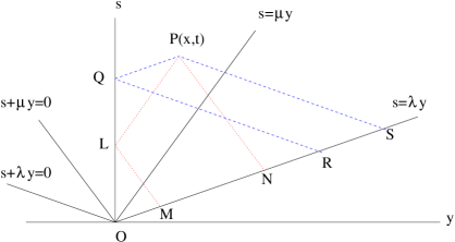
Figure 6: Solution of inhomogeneous wave equation

Now

$$\iint_{PQRS}H_{1} =\frac{1}{2\lambda}\int_{{t-\lambda x}}^{t+\lambda x}\int_{0}^{{t-\lambda x}}H_{1}((q-p)/2\lambda,(q+p)/2)\,dp\,dq,$$ (4.27)

and

$$\iint_{PLMN}H_{2} =\frac{1}{2\mu}\int_{{t-\mu x}}^{t+\mu x}\int_{-(\mu-\lambda)q/(\mu+\lambda)}^{{t-\mu x}}H_{2}((q-p)/2\mu,(q+p)/2)\,dp\,dq$$ (4.28)

with the lower limit of the $q$ integral being $(\mu+\lambda)|t-\mu x|/(\mu-\lambda)$ in the triangular PMN case, that is when $t\leq\mu x$.

If ${\mathbf{H}}$ is continuous on the regions ${0\leq\lambda x\leq t\leq\mu x}$ and ${0\leq\mu x\leq t}$ (but may have jumps across $t=\mu x$) then ${\mathbb{\cal I}}({\mathbf{H}})(x,t)$ is at least $C^{1}$ on each of those regions. Clearly ${\mathbb{\cal I}}({\mathbf{H}})(x,t)$ is continuous on $0\leq\lambda x\leq t$; further, the first component of ${\mathbb{\cal I}}({\mathbf{H}})(x,t)$ is $C^{1}$ on $0\leq\lambda x\leq t$ because its derivatives in directions parallel to $s=\lambda y$ and $s+\lambda y=0$ are the integrals of $H_{1}$ on $PS$ and $PQ$ respectively and these vary continuously with $P$ even across $t=\mu x$. Also, from Figure 6, ${\mathbb{\cal I}}({\mathbf{H}})$ is zero on $x=0$ and $t=\lambda x$. Also, the first order derivatives of the second component of ${\mathbb{\cal I}}({\mathbf{H}})$ on $t=\lambda x$ are zero because the derivatives of the second component, in ${0\leq\lambda x\leq t\leq\mu x}$, in directions parallel $t=\mu x$ and $t+\mu x=c$ are integrals along $PN$ and $PM$ (note $L$ is not present in this case). Finally, if ${\mathbf{H}}$ is $C^{1}$ on the regions ${0\leq\lambda x\leq t\leq\mu x}$ and ${0\leq\mu x\leq t}$ then ${\mathbb{\cal I}}({\mathbf{H}})(x,t)$ is $C^{2}$ on each of those regions. Hence the parts of ${\mathbb{\cal I}}({\mathbf{H}})$ on ${0\leq\lambda x\leq t\leq\mu x}$ and ${0\leq\mu x\leq t}$ are the unique solution of (4.22) - (4.25) when $A=0,B=0$ and ${\mathbf{p}}={\mathbf{q}}={\mathbf{r}}={\mathbf{s}}=0$ with $\{{\mathbf{F}},{\mathbf{G}}\}$ replaced by ${\mathbf{H}}$.

Hence the ${\mathbf{f}},{\mathbf{g}}$ we seek are the solutions of the Volterra like integral equation

$$\{{\mathbf{f}},{\mathbf{g}}\}(x,t)={\mathbb{\cal I}}(\{{\mathbf{F}},{\mathbf{G}}\})(x,t)+{\mathbb{\cal I}}(\{A{\mathbf{f}}_{x}+B{\mathbf{f}},A{\mathbf{g}}_{x}+B{\mathbf{g}}\})(x,t).$$ (4.29)

Fix a $\bar{T}>0$; we wish to solve (4.29) on $D_{\bar{T}}$. For any $T\in(0,\bar{T}]$, let ${\cal B}$ be the Banach space of piecewise vector functions $\{{\mathbf{f}},{\mathbf{g}}\}$ with ${\mathbf{f}}$ a $C^{1}$ function on $L_{T}$ and ${\mathbf{g}}$ a $C^{1}$ function on $U_{T}$ with the $C^{1}$ norms. Now for any ${\mathbf{H}}\in{\cal B}$ we have shown that ${\mathbb{\cal I}}({\mathbf{H}})$ is also in ${\cal B}$; further using (4.27), (4.28), one may show that for $(x,t)\in D_{T}$

$$|{\mathbb{\cal I}}({\mathbf{H}})(x,t)|,~{}|\partial_{t}{\mathbb{\cal I}}({\mathbf{H}})(x,t)|,~{}|\partial_{x}{\mathbb{\cal I}}({\mathbf{H}})(x,t)|{~{}\preccurlyeq~{}}(T+T^{2})\|{\mathbf{H}}\|_{{\cal B}}.$$

Here the derivatives of ${\mathbb{\cal I}}({\mathbf{H}})(x,t)$ and ${\mathbf{H}}(x,t)$ are to be understood to be one sided at points on $t=\mu x$; the constant is determined only by $\lambda,\mu$. Hence we can define the map ${\cal K}$ from ${\cal B}$ to ${\cal B}$ with

$${\cal K}(\{{\mathbf{f}},{\mathbf{g}}\})={\mathbb{\cal I}}(\{{\mathbf{F}},{\mathbf{G}}\})(x,t)+{\mathbb{\cal I}}(\{A{\mathbf{f}}_{x}+B{\mathbf{f}},A{\mathbf{g}}_{x}+B{\mathbf{g}}\})(x,t).$$

For arbitrary $\{{\mathbf{f}},{\mathbf{g}}\}$ and $\{{\mathbf{f}},{\mathbf{g}}\}$ in ${\cal B}$, we may observe that

$$\|{\cal K}(\{{\mathbf{f}},{\mathbf{g}}\})-{\cal K}(\{{\mathbf{f}},{\mathbf{g}}\})\|_{{\cal B}}\leq C(T+T^{2})(|A|_{C(D_{\bar{T}})}+|B|_{C(D_{\bar{T}})})\|\{\tilde{{\mathbf{f}}}-{\mathbf{f}},\tilde{{\mathbf{g}}}-{\mathbf{g}}\}\|_{{\cal B}}$$

with $C$ determined by $\lambda$ and $\mu$, implying ${\cal K}$ is a contraction for $T$ small enough. Hence ${\cal K}$ has a fixed point in ${\cal B}$ and we have proved the existence of the unique solution of (4.29) for $T>0$ small enough.

Now suppose we have solved (4.29) for $T=T_{1}$ for some $0<T_{1}<\bar{T}$; so we have ${\mathbf{f}}^{*},{\mathbf{g}}^{*}$ on $L_{T_{1}}$ which solve (4.29). For any $T\in[T_{1},\bar{T}]$ we redefine ${\cal B}$ as before except that we require that ${\mathbf{f}}={\mathbf{f}}^{*}$ on $L_{T_{1}}$ and ${\mathbf{g}}={\mathbf{g}}^{*}$ on $U_{T_{1}}$. Define ${\cal K}$ as before; then because ${\mathbf{f}}$, ${\mathbf{g}}$ agree with ${\mathbf{f}}^{*}$, ${\mathbf{g}}^{*}$ respectively on $D_{T_{1}}$ and satisfy (4.29) for $T=T_{1}$, one may see that

$$\|{\cal K}(\{\tilde{{\mathbf{f}}},\tilde{{\mathbf{g}}}\})-{\cal K}(\{{\mathbf{f}},{\mathbf{g}}\})\|_{{\cal B}}\leq C(|T-T_{1}|+|T-T_{1}|^{2})(|A|_{C(D_{\bar{T}})}+|B|_{C(D_{\bar{T}})})\|\{\tilde{{\mathbf{f}}}-{\mathbf{f}},\tilde{{\mathbf{g}}}-{\mathbf{g}}\}\|_{{\cal B}}$$

because after the subtraction and the cancelation of the contribution to the integrals over the region $D_{T_{1}}$, the remaining integrals are over subregions of $T_{1}\leq t\leq T$ and no line parallel to $t=\pm\lambda x$ or $t=\pm\mu x$ in this region will have a length exceeding a constant times $T-T_{1}$; the constant determined by $\lambda,\mu$. Hence as before, ${\cal K}$ is a contraction for $T-T_{1}$ small enough. The important point is that there is a positive lower bound on $T-T_{1}$ for which ${\cal K}$ is a contraction and this lower bound is dependent only on $|A|_{C(D_{\bar{T}})}$, $|B|_{C(D_{\bar{T}})}$, $\lambda$, $\mu$ and $\bar{T}$ and is independent of $T_{1}$. So repeating this argument we can construct the solution of (4.29) over $D_{\bar{T}}$.

The solution constructed, $\{{\mathbf{f}},{\mathbf{g}}\}$, is $C^{1}$ on $L_{T}$ and $U_{T}$. However for such $\{{\mathbf{f}},{\mathbf{g}}\}$ the right hand side of (4.29) is $C^{2}$ on $L_{T},U_{T}$. Hence $\{{\mathbf{f}},{\mathbf{g}}\}$ is $C^{2}$ on $L_{T}$ and $U_{T}$.

QED

References

[A87] Achenbach, J. D. Wave propagation in elastic solids, North-Holland Publishing Company, (1987).
[BI06]
Belishev, M. I.; Ivanov, S. A. Reconstruction of the parameters of
a system of connected beams from dynamic boundary measurements.
(Russian) Zap. Nauchn. Sem. S.-Peterburg. Otdel. Mat. Inst.
Steklov. (POMI) 324 (2005), Mat. Vopr. Teor. Rasprostr. Voln.
34, 20–42, 262; translation in J. Math. Sci. (N. Y.) 138
(2006), no. 2, 5491–5502
[BI03]
Belishev, M. I.; Ivanov, S. A. Uniqueness in the small in a
dynamic inverse problem for a two-velocity system. (Russian) Zap.
Nauchn. Sem. S.-Peterburg. Otdel. Mat. Inst. Steklov. (POMI) 275
(2001), Mat. Vopr. Teor. Rasprostr. Voln. 30, 41–54, 310–311;
translation in J. Math. Sci. (N. Y.) 117 (2003), no. 2,
3910–3917
[BI02]
Belishev, M. I.; Ivanov, S. A. Characterization of data in the
dynamic inverse problem for a two-velocity system. (Russian) Zap.
Nauchn. Sem. S.-Peterburg. Otdel. Mat. Inst. Steklov. (POMI) 259
(1999), Kraev. Zadachi Mat. Fiz. i Smezh. Vopr. Teor. Funkts. 30,
19–45, 296; translation in J. Math. Sci. (New York) 109
(2002), no. 5, 1814–1834
[BBI97]
Belishev, M.; Blagovestchenskii, A.; Ivanov, S. The two-velocity
dynamical system: boundary control of waves and inverse problems.
Wave Motion 25 (1997), no. 1, 83–107.
[MNS05]
Morassi, A.; Nakamura, G.; Sini, M. An inverse dynamical problem
for connected beams. European J. Appl. Math. 16 (2005), no. 1,
83–109.
[Ni91]
Nizhnik, L P. Inverse scattering problems for the hyperbolic
equations, Kiev, Naukova Dumka (1991).
[Sa86]
Sacks, P. Computation of the principal part of the linearized map
from coefficients to surface value in the P-SV problem, ONR/SRO
report #36, Department of Theoretical and Applied Mechanics,
Cornell University 1986
[SaSy87] Sacks,P. and Symes, W. Recovery of the elastic parameters of a layered half space, Geophys. J. Roy. Astr Soc. 88, 1987, 593-620.
[SnSy88]
Santosa, F.; Symes, W. High frequency perturbational analysis of
the surface point source response of a layered fluid, J. Comp.
Phys., 74, 1988, 318-381