The secondary eclipse of CoRoT-1b

The transiting planet CoRoT-1b is thought to belong to the $pM$-class of planets, in which the thermal emission dominates in the optical wavelengths. We present a detection of its secondary eclipse in the CoRoT white channel data, whose response function goes from $\sim$400 to $\sim$1000 nm. We used two different filtering approaches, and several methods to evaluate the significance of a detection of the secondary eclipse. We detect a secondary eclipse centered within 20 min at the expected times for a circular orbit, with a depth of 0.016$\pm$0.006%. The center of the eclipse is translated in a 1-$\sigma$ upper limit to the planet’s eccentricity of $e\cos\omega<$0.014. Under the assumption of a zero Bond Albedo and blackbody emission from the planet, it corresponds to a T_CoRoT=2330${}^{+120}_{-140}$ K. We provide the equilibrium temperatures of the planet as a function of the amount of reflected light. If the planet is in thermal equilibrium with the incident flux from the star, our results imply an inefficient transport mechanism of the flux from the day to the night sides.

1 Introduction

When a Hot Jupiter transits its host star, unless the eccentricity is anomalously large, it will also produce secondary eclipses, sometimes also called occultations, from which precious information about the atmospheres of these intriguing objects can be inferred. During the last four years, we have witnessed the first detections of thermal emission from several Hot Jupiters at different band passes in the infrared, most of them from space (Charbonneau et al. 2005; Deming et al. 2005). These pioneering studies have revealed some features of their atmospheres, such as thermal inversions at hight atmospheric altitudes (Knutson et al. 2008, 2009).

The different opacity of the planetary atmosphere, especially due to the abundances of TiO and VO, can make the spectrum emitted by the planet very different, what led Fortney et al. (2008) to propose two classes of exoplanets, $pM$ and $pL$. Those receiving more incident flux from their star, the $pM$ class, would exhibit thermal inversions of their stratospheres, and as a consequence the depths of the secondary eclipses in the optical and near infrared bands will be bigger than expected for a $pL$ planet. These authors, as well as López-Morales & Seager (2007), argue that in the red parts of the optical spectrum, the thermal emission from these objects is much more important than the contribution of the reflected light, as theoretical models are in agreement with a very low albedo $A$ for $pM$ planets (Sudarsky et al. 2000; Burrows et al. 2008; Hood et al. 2008).

The first transiting planet detected from space, CoRoT-1b (Barge et al., 2008), completes an orbit around its G0V star every 1.5 d. Its incident flux puts this planet in the $pM$ category. In this paper, we focus on the detection of its secondary eclipse. We describe the data set and the preparation of the light curve for the search for the secondary in Section 2, and the different techniques used to evaluate the significance and depths of the secondary in Section 3. Finally, in Section 4, we discuss the physical implications of our results.

2 Observations

CoRoT-1b was observed during the first observing run of CoRoT, attaining a total duration of 52.7 d. In the present study, the photometry was performed using the latest version of the pipeline, which uses the information about the instrument’s Point Spread Function and the centroids of the stars measured in the asteroseismic channel to correct for the effects of the satellite jitter in the white light curve. The effect of the Earth eclipses, in which a thermal shock is translated in a bigger jitter and thus less flux inside the photometric apertures, is greatly improved in this new version of the pipeline.

The light curve was sampled every 512 s for the first 28 days, and then changed to 32 s until the end of the run. During the 512 s part, the dispersion of the normalized data is 0.00079, and 0.0019 in the 32 s section. The pipeline version of the light curve is plotted in Fig. 1. To evaluate the red noise content in our data (e.g. Pont et al. 2006), we computed the standard deviation of the light curve (filtered with a median filter with a window of 12 h) with different bin sizes, ranging from 30 to 500 min. The result is plotted in Fig. 2; the 32-s part of the curve shows less noise than the 512-s part below bins of $\sim$150 min, while it achieves similar levels as the 512-s part above that size. This reveals the presence of uncorrected low frequencies at levels of $<$10^-4 in units of normalized flux, and of uncorrected signals of about 2$\times$10^-4 with periods between 30 and 150 min in the 512-s part of the data.

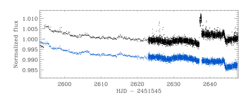
Figure 1: Light curve of CoRoT-1b prepared for secondary eclipse search (the transits have been removed). For displaying purposes, the data were combined in 10-points bins. The black points show the pipeline version of the curve, while the blue points show the curve corrected for the orbital residuals, hot pixels and remaining outliers, as described in the text.

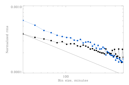
Figure 2: The standard deviation of the light curve after removing a median filtered version with a 12-h window, and after combining it in bins of different sizes. Black dots are for the 32-s part of the light curve, and blue dots for the 512-s part. The solid line follows the theoretical diminution of the dispersion from the 30 min point in the 32-s part, if the noise were white.

3 Analysis of the CoRoT light curve

We present two different analysis of the data in order to search and measure the secondary eclipse of CoRoT-1b. They differ substantially from the preparation of the light curve to the estimation of the significance of the secondary eclipse detection, and we considered both in order to reinforce or invalidate a detection of the secondary eclipse.

3.1 First analysis: filtering, local polynomial normalization and trapezoid fit

Two jumps in the data, due to hot pixels, were corrected by estimating the median fluxes before and after the jump, and we rejected the points belonging to the region between CoRoT date (HJD - 2451545) 2637.1 and 2637.75, as they were affected by the stabilization of the hot pixel to its normal levels.

Figure 3: Amplitude spectrum of the light curve of CoRoT-Exo-1, before (left) and after (right) the correction for the orbital residuals described in the text.

The signal we want to measure is at the 10^-4 level, and thus we inspected the level of noise in the light curve by producing its amplitude spectrum using Period04 (Lenz & Breger, 2005). In the left panel of Fig. 3, some peaks at the orbital frequency and its daily aliases remain at a level of $1.5\times 10^{-4}$. This motivated us to try to improve the filtering at the orbital period. We estimated the signal at each satellite’s orbit $i$ from the signal in the 30 orbits before and after the orbit $i$, as described in Alonso et al. (2008). Some remaining outliers were located by subtracting the low frequencies in the curve using a moving median filter with a window of about 1 d, and flagging iteratively the points at more than 3 times the standard deviation calculated in a robust way. Finally, these points were replaced by interpolations to their closest points. In total, these interpolated points represent 3.0% of the original data. The amplitude spectrum of the corrected curve is plotted in the right panel of Fig. 3, where the amplitudes of the peaks at the orbital frequency and its aliases and overtones have clearly been reduced.

To avoid possible effects of unequal number of points at different orbital phases due to the phases at the beginning and end of the observations, we cut the parts of the data before the first recorded transit and after the last one. As we are interested in the secondary eclipse, we also cut the transits in the curve. The light curve prepared for the search for the secondary eclipse is plotted in Fig. 1.

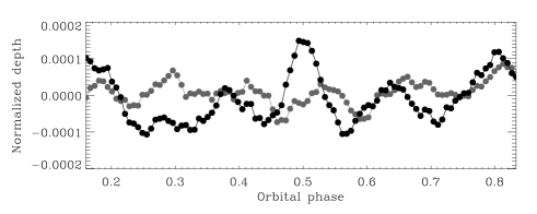
Figure 4: Depth of a trapezoid with the shape and duration of a transit, as a function of the planet’s orbital phase. The maximum is centered in phase 0.5, corresponding to the secondary eclipse. In grey, the result in a light curve where the secondary eclipse signal has been diluted (see text for details).

Figure 5: Phase folded curve of CoRoT-1b during the phases of secondary eclipse. The data have been binned in 0.01 in phase ($\sim$22 min).

Figure 6: The $\chi^{2}$ space for different centers and depths of the secondary eclipse, and the different $\sigma$ confidence limits.

Figure 7: The $\chi^{2}$ for the duration of the secondary eclipse, and the 1,2 and 3$\sigma$ confidence limits. The vertical line shows the total duration of a transit. The detected signal has the same duration as the transit at 1-$sigma$ level.

For the search of the secondary eclipse, we followed the method described in Alonso et al. (2009a). Basically, it consists in evaluating the depths of fits to trapezoids with the same overall shape as the planet’s transit, at different phases of the orbital period. At each test phase $\phi_{i}$, the low frequencies are removed by performing, at each planetary orbit, linear fits to the regions $[\phi_{i}-\phi_{a}-\phi_{b},\phi_{i}-\phi_{a})\bigcup(\phi_{i}+\phi_{a},\phi_{i}+\phi_{a}+\phi_{b}]$, where $\phi_{a}$ and $\phi_{b}$ were chosen in order not to include points inside a transit duration, but at the same time allowing enough data points to enter in the fit. We obtained a good compromise using the values $\phi_{a}$= 0.04 and $\phi_{b}$=0.12. Once all the planetary orbits were normalized this way, we binned the data with a size of 0.001 in phase, and fitted the depth of a trapezoid using a Levenberg/Marquardt algorithm (Levenberg 1944; Marquardt 1963), fixing the rest of the trapezoid’s parameters to the values of the transit. The final depth of the fits as a function of the orbital phase is plotted in Fig. 4, where the maximum is well centered at the expected orbital phase 0.5. We can evaluate the significance of this detection by computing the dispersion of the fitted depths in the parts of the phase diagram not affected by the inclusion of the secondary eclipse at phase 0.5 in the regions where the fits used to normalize the transits were computed, i.e., $\phi\in[0,0.5-\phi_{a}-\phi_{b})\bigcup(0.5+\phi_{a}+\phi_{b},1]$. The significance of the detection calculated this way results in 2.1-$\sigma$. The phase folded light curve around the secondary phase and the best fit trapezoid (with duration and shape fixed to that of the transits) are shown in Fig. 5.

We performed the same technique in a light curve where we diluted the signal of the secondary eclipse. To do so, we subtracted from the light curve a version of it, filtered with a moving median using a window of $\sim$1 d in duration. We shuffled randomly the residuals, and we added back the subtracted filtered curve. The resulting depth vs. phase diagram using the method described above in this curve is plotted as a grey line in the Fig. 4. If we take the dispersion of this measured depth (3.29$\times$10^-5) as the precision in the measurement of the secondary eclipse, then the significance of the signal at phase 0.5 is 4.5-$\sigma$.

Additionally, three different methods to evaluate the depth and significance of the secondary eclipse signal were tested. In the first method, we removed the best fit trapezoid to the data (where the only fitted parameter was the depth, the rest was fixed to the values of the transit), shifted circularly the residuals, reinserted the signal, and re-evaluated the fitted depth. The final depth thus takes into account the effect of red noise in the data, and it is of 0.014$\pm$0.002%. The second method consisted in fitting two gaussians to 1) the distribution of points inside total eclipse and 2) a subset of the points outside the eclipse with the same number of points as in 1), and compare their fitted centers. This fit was performed to 500 subsets of 2), with a randomly chosen starting point and varying the size of the bins in the distribution between 0.005% and 0.02%. The result is of 0.021$\pm$0.003%. In the third method, we explored the $\chi^{2}$ distribution in a grid of centers (from -60 to +60 minutes from the expected center) and depths (from 0.01% to 0.04%) of the secondary eclipse. The other parameters of the trapezoid were fixed to the values of the transit. The minimum $\chi^{2}$ and the 1,2 and 3-$\sigma$ confidence levels are presented in Fig. 6, and the best fitted depth using this method is 0.016$\pm$0.006%. We show the $\chi^{2}$ map of the duration of the trapezoid and the 1,2,3-$\sigma$ confidence levels in Fig. 7. The duration of the secondary eclipse is, as expected, compatible at a $<$2-$\sigma$ level with the duration of the transits.

3.2 Second analysis: using the IRF filter

The analysis presented so far shows encouraging evidence for the detection of a secondary eclipse at the expected phase and duration for a circular or almost circular orbit. However, the detection is unavoidably tentative given the extremely shallow nature of the signal. Each step of the analysis involved a number of free parameters, from the hot pixel and satellite orbit residual corrections to the individual corrections applied for stellar variability local to each putative secondary location.

In an effort to reinforce or invalidate the detection, we carried out a separate secondary eclipse search using different pre-processing and eclipse detection methods which were designed to minimize the number of free parameters. The regions around the hot pixel events were simply clipped out, no correction for orbital residuals was applied, and we used the iterative reconstruction filter (IRF) of Alapini & Aigrain (2009), which has only two free parameters, to isolate signal at the planet’s orbital period from other signals including stellar variability.

The starting point of this analysis was the same light curve, as described in Section 2. To circumvent the issue of varying data weights associated with different time sampling, the oversampled section of the light curve was rebinned to 512s sampling. Outliers were then identified and clipped out using a moving median filter (see Aigrain et al. 2009 for details). Finally, we also discarded two segments of the light curve, in the CoRoT date ranges 2594.25–2594.45 and 2637.10–2637.70), corresponding to the two hot pixel events visible in Fig. 1. This last step was necessary as the IRF cannot remove the sharp flux variations associated with hot pixels without affecting the transit signal.

The resulting time-series was then fed into the IRF. A full description of this filter is given in Alapini & Aigrain (2009), but we repeat the basic principles of the method here for completeness. The IRF treats the light curve $\{Y(i)\}$ as $Y(i)=F(i)\,A(i)+R(i)$, where $\{A(i)\}$ represents the signal at the period of the planet, which is a multiplicative term applied to the intrinsic stellar flux $\{F(i)\}$, and $\{R(i)\}$ represents observational noise. A first estimate of $\{A(i)\}$ is obtained by folding the light curve at the period of the transit and smoothing it using a smoothing length of 0.0006 in phase, and is divided into the original light curve. This is then run through an iterative non-linear filter (Aigrain & Irwin, 2004) which preserves signal at frequencies longer than 0.5 days to give an estimate of the stellar signal $\{F(i)\}$, which is assumed to be primarily concentrated on relatively long time-scales. This signal in turn is removed from the original light curve and the process is iterated until the the dispersion of the residuals remains below $10^{-4}$ for 3 consecutive iterations, which occurs after 3 iterations in this case.

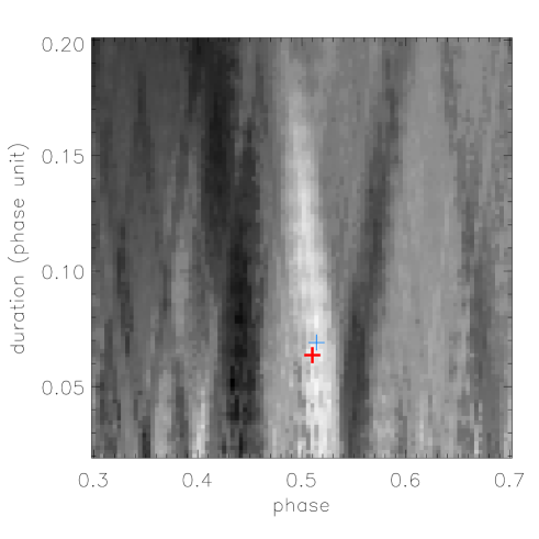
Figure 8: Detection significance map. The red thick cross is the secondary eclipse duration and phase with the largest detection significance. The blue thin cross is the largest detection significance for a secondary eclipse of the same duration as the primary transit.

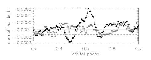
Figure 9: Depth of a box as a function of the planet s orbital phase (black curve) with the total eclipse duration (0.0697 in phase units) providing the highest detection significance. The largest significance is found for a secondary eclipse depth of 0.019% at an orbital phase of 0.510. The grey dashed lines show the scatter ($\pm$0.006%) of depths measured in a light curve freed from the secondary eclipse with shuffled residuals (grey curve). This scatter is an estimate of the uncertainty on the depth measurements.

The free parameters of the IRF are the smoothing lengths used when estimating $\{A(i)\}$ and $\{F(i)\}$. The former represents a compromise between reducing the noise and blurring out potential sharp features associated with the planet, and the latter between removing the stellar signal without affecting the planetary signal. The values chosen here were adopted by trial and error and gave the best results when evaluating the performace of the IRF for transit reconstruction purposes (Alapini & Aigrain, 2009).

We searched the IRF-filtered light curve for secondary eclipses using a very simple sliding box algorithm, where the model is taken to be 1 outside the eclipse and the in-eclipse level is set to the median of the in-eclipse points (the light curve was previously normalised by dividing it be the median of the out-of-transit points). This is therefore a 2-parameter model, and the phase and duration of the eclipse were varied over a $100\times 100$ grid ranging from 0.3 to 0.7 in phase and from 0.02 to 0.2 in duration, where the duration is measured in phase units (corresponding to 0.7 to 7.2 hours). We then evaluate the significance of the detection, in arbitrary units, by dividing the eclipse depth by $\sigma/\sqrt{(}N)$, where sigma is the scatter of the points - outside the primary transit - in the IRF-filtered light curve and $N$ is the number of point used to calculate the level inside the secondary eclipse. The resulting confidence map is shown in Fig. 8, where the phase and duration giving the best significance are marked with a red cross. The best duration corresponds almost exactly to the full duration of the transit (which we measure as 0.0688 in phase units from a trapezoidal fit), and the best phase is 0.510, in good agreement with the results of Fig. 6. The diagonal patterns in the significance map are due to individual features in the folded, filtered light curve, which influence a wider range of trial phases at longer durations.

Fig. 9 shows the eclipse depth as a function of orbital phase at the best duration. The best-fit depth is 0.019%, consistent with the results presented above. One should bear in mind when comparing the different results that the eclipse depth was measured here relative to the overall median flux rather than to a local estimate of the out-of-eclipse flux.

To calculate the significance of the detection, we measured the depth and associated uncertainty and divided the former by the latter. In this case, we calculated the uncertainty as the dispersion (estimated as 1.48$\times$MAD) around the median level of the light curve outside the primary transit, and divided this value by the square root of the number of points inside the secondary eclipse. This results in an uncertainty of 0.005%, i.e. a 3.5 $\sigma$ detection. We also applied the three other methods already presented in Section 3.1. All of these give an uncertainty estimate of 0.006%, which we adopt as the final uncertainty on the eclipse depth derived from the IRF.

The fact that we arrived at consistent estimates of the secondary eclipse depth and significance using different approaches to filter the light curve and evaluate the uncertainty on the depth lends confidence to the detection. Our final adopted values for the depth is 0.016$\pm$0.006%, consistent with all our estimates within one sigma. The eclipse center occurs at the expected phase for a circular orbit, with an uncertainty of about 20 min.

4 Discussion

We have shown that a decrease in the flux of the light curve of CoRoT-1b at the phases of secondary eclipse is detected at more than 3-$\sigma$ level. Its duration is, within 1-$\sigma$, the same as the duration of the transits, and its shallow depth is of only 0.016$\pm$0.006%. We thus interpret this signal as the secondary eclipse, detected at the optical part of the spectrum.

If we were to explain the secondary eclipse detection as reflected light, it would imply a geometric albedo of $A_{g}$=0.20$\pm$0.08, which is a bigger value than several upper limits provided by other works in different exoplanets (Collier Cameron et al. 2002; Rowe et al. 2008). Furthermore, theoretical models predict a strong optical absorption in the Hot Jupiters’ atmospheres (e.g. Sudarsky et al. 2000; Burrows et al. 2008; Hood et al. 2008), and for the $pM$-class of planets, thermal emission dominates by more than an order of magnitude the reflected light. Consequently, we suspect that the secondary eclipse signature is not produced entirely by reflected light, but most probably by a combination of thermal emission and some reflected light, as in the case of CoRoT-2b (Alonso et al., 2009b).

The CoRoT bi-prism allows to recover chromatic information from the signal. In this case, the difference between the significance of the secondary signal in the blue and the red channels might clarify if our detected signal is dominated by reflected light or by thermal emission in the optical, as we assumed given the arguments above. In the first case, the secondary should be detected mostly in the blue channel, while in the case of thermal emission the red channel would carry most of the signal. We checked the colors in the CoRoT-1 aperture, but unfortunately the residuals of the jitter correction and the noisier individual channels did not allow us to conclude on this subject.

The equilibrium temperature can be calculated as

$$T_{eq}=T_{\star}(R_{\star}/a)^{1/2}[f(1-A_{B})]^{1/4}$$ (1)

which depends on the Bond albedo $A_{B}$ and the re-distribution factor $f$ which accounts for the efficiency of the transport of energy from the day to the night side of the planet. $f$ can vary between $1/4$ for an extremely efficient redistribution (isothermal emission at every location of the planet) and higher values for an inefficient redistribution, implying big differences in the temperatures at the day/night sides of the planet.

To translate the measured depth of the secondary eclipse into brightness temperatures, we used a theoretical model of a G0V star from the Pickles library of stellar models (Pickles, 1998), calibrated in order to produce the same integrated flux as a Planck black-body spectrum with a T_eff=5950 K. Under the assumption that the planetary emission is well reproduced by a black-body spectrum, and as we know the ratio R_p/R_⋆ from the transits, we can calculate the temperatures that produce secondary eclipse depths compatible with our result, using the CoRoT response function given in Auvergne et al. (2009). The brightness temperature calculated this way resulted in T_CoRoT=2330${}^{+120}_{-140}$ K. If we further assume that the planet is in thermal equilibrium and a zero Bond Albedo, this temperature favors high values of the re-distribution factor $f$=0.57${}^{+0.10}_{-0.13}$. A diagram showing the implied equilibrium temperatures as a function of the albedo, where we have assumed for simplicity that all the reflected light is detected in the white channel of CoRoT (i.e., that $A_{g}$=$A_{B}$, as in Alonso et al. 09b) is shown in Fig. 10.

Figure 10: The implied equilibrium temperatures from the secondary eclipse measurement, as a function of the amount of reflected light. The best fitted depth and the one sigma limits are plotted as the solid lines. Different values of the re-distribution factors as defined by Eq. 1 are plotted as dotted lines. Zero albedo solutions imply high values of the re-distribution factor.

Non-zero Bond Albedos, where some of the detected flux is reflected light from the star, would imply smaller values of $f$, whilst solutions with A$>$0.30 are not compatible with the measured secondary eclipse. All the solutions with equilibrium temperatures higher than 1900 K are for $f$ values bigger than 1/4. Thus, the secondary eclipse detection favors inefficient redistributions of the incident flux from the day to the night side.

One may wonder if the $k=R_{pl}/R_{\star}$ obtained from the transit fit should be different because of the lack of inclusion of the emitted light from the planet in the model. Even for an extreme case of $f=1/4$, the correction to be applied on the $k$ is a factor of 3 below the uncertainty given in Barge et al. (2008), and thus we do not consider it necessary.

The measured center of the secondary eclipse, with an uncertainty of 20 min, can be used to constrain the $e\cos\omega<$0.014 at a 1-$\sigma$ level.

Our measured brightness temperature can be used to predict eclipse depths in the $K_{s}$ and $z$ bands of 0.25% and 0.014% respectively. In these bands, ground-based observations have recently been successful in the detections of secondary eclipses of exoplanets (Sing & López-Morales 2009; de Mooij & Snellen 2009), and for the case of CoRoT-1b, the observations might reveal departures from the black-body assumption such as the thermal inversions observed in several planets (e.g. Knutson et al. 2008, 2009).