Balancing the vacuum energy in heterotic $M$-theory

Abstract

Moduli stabilisation is explored in the context of low-energy heterotic $M$-theory to show that a small value of the cosmological constant can result from a balance between the negative potential energy left over from stabilising the moduli and a positive Casimir energy from the higher dimensions. Supersymmetry breaking is induced by the fermion boundary conditions on the two branes in the theory. An explicit calculation of the Casimir energy for the gravitino reveals that the energy has the correct sign, although the size of the contribution is close to the edge of the parameter range for which the calculation is valid.

I introduction

Horava and Witten Horava and Witten (1996a, b) proposed some time ago that the low-energy limit of strongly coupled $E_{8}\times E_{8}$ heterotic string theory could be formulated as eleven dimensional supergravity on a manifold with boundary. This was an important step on the road to $M$-theory, and heterotic $M$-theory is now regarded as one of the low-energy limits of $M$-theory and a possible link between $M$-theory and particle phenomenology Witten (1996); Banks and Dine (1996).

The original formulation of heterotic $M$-theory was based on 11-dimensional supergravity and then built up order by order as a series in a small parameter $\epsilon\sim\kappa_{11}{}^{2/3}$ depending on the gravitational coupling $\kappa_{11}$. At the next order came two 10-dimensional boundary terms with $E_{8}$-Yang-Mills matter multiplets. Unfortunately, at higher orders the theory became ill-defined. This problem was resolved several years later by a simple modification to the boundary conditions, resulting in a low-energy effective theory which is supersymmetric to all orders. We shall be using this improved version of heterotic $M$-theory, described in Refs. Moss (2003, 2005, 2006, 2008).

For applications to particle phenomenology, six of the internal dimensions lie on a deformed Calabi-Yau manifold and one internal dimension stretches between the two boundaries containing the matter fields Witten (1996); Banks and Dine (1996); Lukas et al. (1999a, b). A variety of mechanisms have been proposed for stabilising the large number of moduli resulting from this compactification:

• internal fluxes, which might fix the $(2,1)$ type of Calabi-Yau moduli by analogy with the moduli stabilisation used in type IIB string theory Kachru et al. (2003a, b)

• membranes stretching between the boundaries, which contribute to fixing the $(1,1)$ type of Calabi-Yau moduli Curio and Krause (2002); Buchbinder and Ovrut (2004); Braun and Ovrut (2006)

• gaugino condensation, which contributes to fixing the Calabi-Yau volume Dine et al. (1985); Horava (1996); Lukas et al. (1998); Becker et al. (2004); Gray et al. (2007)

In addition to the moduli stabilisation, an ‘uplifting’ mechanism has to be found which makes the effective cosmological constant non-negative Kachru et al. (2003b). Fully consistent reductions of heterotic $M$-theory have been constructed along these lines, with anti-5-branes providing an uplifting mechanism Braun and Ovrut (2006). These reductions have also taken advantage of the extra flexibility allowed by the inclusion of 5-branes.

In this paper we explore the possibility that the small value of the cosmological constant results from a balance between the negative potential energy left over from stabilising the moduli and a positive Casimir energy from the higher dimensions. To be more specific, we use the difference in Casimir energy between a supersymmetric state and a broken symmetry state, because differences in vacuum energy can be calculated more reliably using only the low energy effective theory.

Some form of supersymmetry breaking is required by any uplifting mechanism, and the possibility we consider is that the fermion chirality condition is different on the two boundaries. This type of supersymmetry breaking was first introduced into heterotic $M$-theory by Antoniadis and Queros Antoniadis and Quiros (1997). They argued that modifying the fermion boundary conditions was analagous to introducing a gaugino condensate into the weakly coupled superstring theory. The new formulation of heterotic $M$-theory Moss (2003, 2005, 2006, 2008) makes the link between gaugino condensation and the boundary conditions on the fermion fields explicit, so that this type of supersymmetry breaking is realised spontaneously whenever a gaugino condensate is present.

In the past, Casimir energy contributions have been widely used to fix the values of radion modulus field in brane-world models Toms (2000); Garriga et al. (2001, 2003); Flachi et al. (2003). These calculations have also been extended to models with modified fermion boundary conditions Fabinger and Horava (2000); Flachi et al. (2001a, b). In the present work, the Casimir force between the branes is relatively small compared to the moduli stabilisation effects described above, but the Casimir vacuum energy has a similar scale to the negative potential energy. Just as with the type IIB superstring Kachru et al. (2003b), one of the parameters in the theory has to be fine-tuned to obtain a small cosmological constant.

The relevant features of the new formulation of heterotic $M$-theory are described in the next section, where we also consider the backgrounds and moduli for the reduced theory. Moduli stabilisation and the vacuum energy are covered in Sect. III. A calculation of the Casimir energy for the gravitino is done in Sect. IV.

In this paper, the 11-dimensional coordinate indices are denoted by $I,J,\dots$, and the coordinate indices on the boundary are denoted by $A,B,\dots$ with the outward normal index by $N$. Otherwise, conventions generally follow Green, Schwarz and Witten Green et al. (1987). In particular, the 11-dimensional gamma matrices satisfy $\{\Gamma_{I},\Gamma_{J}\}=2g_{IJ}$, where the metric signature is $-+\dots+$. In the reduced theory, four dimensions are indicated by $\mu,\nu\dots$ and the fifth by $z$.

II Heterotic $M$-theory

Heterotic $M$-theory is formulated on a manifold ${\cal M}$ with a boundary consisting of two disconnected components ${\cal M}_{1}$ and ${\cal M}_{2}$. The eleven-dimensional part of the action is conventional for supergravity,

$$S_{SG}= {1\over 2\kappa_{11}^{2}}\int_{\cal M}\left(-R(\Omega)-\bar{\Psi}_{I}\Gamma^{IJK}D_{J}(\Omega^{*})\Psi_{K}-\frac{1}{24}G_{IJKL}G^{IJKL}\right.$$ (1)

$$\left.-\frac{\sqrt{2}}{96}\left(\bar{\Psi}_{I}\Gamma^{IJKLMP}\Psi_{P}+12\bar{\Psi}^{J}\Gamma^{KL}\Psi^{M}\right)G^{*}_{JKLM}-\frac{2\sqrt{2}}{11!}\epsilon^{I_{1}\dots I_{11}}(C\wedge G\wedge G)_{I_{1}\dots I_{11}}\right)dv,$$

where $\Psi_{I}$ is the gravitino, $G$ is the abelian field strength and $\Omega$ is the tetrad connection. The combination $G^{*}=(G+\hat{G})/2$, where hats denote the standardised subtraction of gravitino terms to make a supercovariant expression.

The boundary terms which make the action supersymmetric are Luckock and Moss (1989),

$$S_{0}={1\over\kappa_{11}^{2}}\int_{\cal\partial M}\left(\hat{K}\mp\frac{1}{4}\bar{\Psi}_{A}\Gamma^{A}\Gamma^{B}\Psi_{B}\right)dv,$$ (2)

where $K$ is the extrinsic curvature of the boundary. We shall take the upper sign on the boundary component ${\cal M}_{1}$ and the lower sign on the boundary component ${\cal M}_{2}$.

For an anomaly-free theory, we have to include further boundary terms with $E_{8}$-Yang-Mills multiplets

$$S_{YM}=-{\epsilon\over\kappa_{11}^{2}}\int_{\cal\partial M}\left(\frac{1}{4}{\rm tr}F^{2}+\frac{1}{2}{\rm tr}\bar{\chi}\Gamma^{A}D_{A}(\hat{\Omega}^{**})\chi+\frac{1}{4}\bar{\Psi}_{A}\Gamma^{BC}\Gamma^{A}{\rm tr}{F}^{*}_{BC}\chi\right)dv,$$ (3)

where $\Omega^{**}=(\Omega+\Omega^{*})/2$. The original formulation of Horava and Witten contained an extra ‘$\chi\chi\chi\Psi$’ term, but this term is not present in the new version. The new theory also has boundary terms depending on $R^{2}$ Moss (2008).

The specification of the theory is completed by a supersymmetric set of boundary conditions. For the tangential anti-symmetric tensor components Moss (2005, 2008),

$$C_{ABC}=\mp\frac{\sqrt{2}}{12}\epsilon\,\left(\omega^{Y}_{ABC}-\frac{1}{2}\omega^{L}_{ABC}\right)\mp\frac{\sqrt{2}}{48}\epsilon\,{\rm tr}\bar{\chi}\Gamma_{ABC}\chi.$$ (4)

where $\omega^{Y}$ and $\omega^{L}$ are the Yang-Mills and Lorentz Chern-Simons forms respectively. These boundary conditions replace a modified Bianchi identity in the old formulation. A suggestion along these lines was made in the original paper of Horava and Witten Horava and Witten (1996b). Boundary conditions on the gravitino are,

$$\Gamma^{AB}\left(P_{\pm}\pm\epsilon\Gamma P_{\mp}\right)\Psi_{A}=\pm\epsilon\left(J_{Y}{}^{A}-\frac{1}{2}J_{L}{}^{A}\right),$$ (5)

where $P_{\pm}=(1\pm\Gamma_{N})/2$ project onto chiral spinors (using the outward-going normals) and

$$\Gamma=\frac{1}{96}{\rm tr}(\bar{\chi}\Gamma_{ABC}\chi)\Gamma^{ABC}.$$ (6)

$J_{Y}$ is the Yang-Mills supercurrent and $J_{L}$ is a gravitino analogue of the Yang-Mills supercurrent.

The resulting theory is supersymmetric to all orders in the parameter $\epsilon$ when working to order $R^{2}$ in the curvature. The gauge, gravity and supergravity anomalies all vanish if

$$\epsilon={1\over 4\pi}\left({\kappa_{11}\over 4\pi}\right)^{2/3}.$$ (7)

Further details of the anomaly cancellation, and additional Green-Schwarz terms, can be found in Ref. Moss (2006).

II.1 Background

Reduction of low-energy heterotic $M-$theory to $4$-dimensions follows a traditional route, where the light fields in the $4-$dimensional theory correspond to the moduli of a background solution in $11$-dimensions. The anzatz for the background metric is based on a warped product $M\times S^{1}/Z_{2}\times Y$ where $Y$ is a Calabi-Yau space Witten (1996); Lukas et al. (1999a, b, c). Since $S^{1}/Z_{2}$ is topologically the same as a finite interval, there are two copies of the $4-$dimensional manifold $M$, the visible brane $M_{1}$ and the hidden brane $M_{2}$, separated by a distance $l_{11}$. A typical value for the inverse radius of the Calabi-Yau space would be of order the Grand Unification scale $10^{16}$GeV and the inverse separation would be of order $10^{14}$GeV.

The background solutions are only determined order by order in $\epsilon$. The improved version of heterotic $M$-theory, which starts from an action which is valid to all orders in $\epsilon$, gives better control of the error terms than previous versions of the theory. We shall follow Ref. Ahmed and Moss (2008) for the reduction, and further details can be found in that reference.

The explicit form of the background metric anzatz which we shall use is

$$ds^{2}=V^{-2/3}dz^{2}+V^{-1/3}\Phi^{2}\tilde{g}_{\mu\nu}dx^{\mu}dx^{\nu}+V^{1/3}(\tilde{g}_{a\bar{b}}dx^{a}dx^{\bar{b}}+\tilde{g}_{\bar{a}b}dx^{\bar{a}}dx^{b}),$$ (8)

where $\tilde{g}_{a\bar{b}}$ a fixed metric on $Y$ and $V\equiv V(z,x^{\mu})$, $z_{1}\leq z\leq z_{2}$ is related to both the volume of the Calabi-Yau space and the warping of the 5-dimensional part of the metric. Our background metric anzatz is similar to one used by Curio and Krause Curio and Krause (2001), except that we use a different coordinate $z$ in the $S^{1}/Z_{2}$ direction. The factor $\Phi^{2}$ is required to put the put the metric $\tilde{g}_{\mu\nu}$ on $M$ into the Einstein frame.

Initially, we restrict the class of Calabi-Yau spaces to those with only one harmonic $(1,1)$ form, $h_{1,1}=1$. In this case the background flux for the antisymmetrc tensor field depends on only one parameter $\alpha$,

$$G^{0}_{ab\bar{c}\bar{d}}=\frac{1}{3}\alpha\left(\tilde{g}_{a\bar{c}}\tilde{g}_{b\bar{d}}-\tilde{g}_{a\bar{d}}\tilde{g}_{b\bar{c}}\right)$$ (9)

This anzatz solves the field equation $\nabla\cdot G^{0}=0$. The boundary conditions (4) are satisfied if there is a non-zero Yang-Mills flux on the hidden brane and,

$$\alpha={4\sqrt{2}\pi^{2}\over v_{CY}^{2/3}}\epsilon\beta$$ (10)

where $v_{CY}$ is the volume of the Calabi-Yau space and $\beta$ is an integer characterising the Pontrjagin class of the Calabi-Yau space.

The volume function $V(z)$ is determined by the exact solution of the ‘$zz$’ component of the Einstein equations ,

$$V(z)=1-\sqrt{2}\alpha z.$$ (11)

The background metric is then consistent with all of the Einstein equations apart from the ones with components along the Calabi-Yau direction, where the Einstein tensor vanishes but the stress energy tensor is $O(\alpha^{2})$. The difference between an exact solution to the Einstein equations and the metric anzatz $\delta g_{IJ}=O(\alpha^{2})$. If we calculate the action to reduce the theory to four dimensions, then the error in the action is $O(\alpha^{4})$. As long as we work within this level of approximation we can use the Calabi-Yau approximation as the background for our reduced theory. Note that this approximation is uniform in $z$, and having small values of $\alpha$ does not necessarily mean small values of $\alpha z$.

This background metric generalises for any internal Calabi-Yau space and accordingly is known as the universal solution Lukas et al. (1999b). The $h_{1,1}$ integers $\beta_{i}$ which characterise the Pontrjagin class of the Calabi-Yau space can be combined into a single parameter $\beta$, defined by

$$\beta=(\beta^{i}\beta_{i})^{2/3}$$ (12)

where $d_{ijk}\beta^{i}\beta^{j}=6\beta_{i}$ and $d_{ijk}$ are Calabi-Yau intersection numbers. The parameter $\alpha$ is defined by Eq. (10). Generally, $\beta$ is not an integer, but most examples have $\beta\geq 1$. In cases where $h_{1,1}>1$ there are other solutions with different functional behaviour for $V(z)$ but we shall only consider the universal solution.

We shall be focussing especially on two moduli of the 4-dimensional theory, the values of $V$ on the two boundaries, $V_{1}$ and $V_{2}$. When $V_{1}$ and $V_{2}$ depend on $x^{\mu}$, the factor $\Phi^{2}$ required to put the metric $\tilde{g}_{\mu\nu}$ into the Einstein frame is,

$$\Phi=\left(V_{1}^{4/3}-V_{2}^{4/3}\right)^{-1/2}.$$ (13)

With this definition of the Einstein metric, the gravitational coupling in 4 dimensions is given by

$$\kappa_{4}^{2}={4\sqrt{2}\over 3}{\kappa^{2}_{11}\over v_{CY}}\alpha.$$ (14)

The reduction to 4 dimensions has also been done using a superfield formalism by Correia et al Paccetti Correia et al. (2006). This shows that in the $h_{1,1}=1$ case the reduced theory is a supergravity model with $V_{1}$ and $V_{2}$ belonging to chiral superfields $S_{1}$ and $S_{2}$ with Kahler potential

$$K=-3\ln\left((S_{1}+S_{1}^{*})^{4/3}-(S_{2}+S_{2}^{*})^{4/3}\right)$$ (15)

Note that, for the real scalar components, the conformal factor introduced in Eq. (8) and the Kahler potential are related by

$$\Phi=2^{2/3}e^{K/6}.$$ (16)

In the weakly-coupled superstring limit, which corresponds to small brane-separation, $S_{1}\approx S+\alpha T/\sqrt{2}$ and $S_{2}\approx S-\alpha T/\sqrt{2}$, where $S$ and $T$ are heterotic superstring moduli.

II.2 Energy scales

The metric anzantz for the universal solution can also be used in the Yang-mills action on the boundary $\partial{\cal M}$,

$$S_{YM}=-{\epsilon v_{CY}\over 2\kappa_{11}^{2}}\int_{\partial\cal M}\frac{1}{4}V{\rm tr}(F^{2})d\tau.$$ (17)

This suggests that the grand-unification fine-structure constant is related to a parameter $\alpha_{GUT}$,

$$\alpha_{GUT}={\kappa_{11}^{2}\over 8\pi\epsilon v_{CY}}.$$ (18)

(The grand-unification fine-structure constant is actually $\alpha_{GUT}/V_{1}$). Eqs. (7), (14), (10) and (18) allow all of the model parameters $\kappa_{11}$, $\epsilon$, $\alpha$ and $v_{CY}$ to be expressed in terms of the topological parameter $\beta$, the Planck length $\kappa_{4}$ and the fine-structure parameter $\alpha_{GUT}$:

$$v_{CY}^{-1/6} = \left(2\over 3\pi\right)^{1/2}\beta^{1/2}\alpha_{GUT}\kappa_{4}^{-1}$$ (19)

$$\kappa_{11}^{-2/9} = \left(2\over 3\pi\right)^{1/2}\left({\sqrt{2}\pi}\right)^{-1/9}\beta^{1/2}\alpha_{GUT}^{5/6}\kappa_{4}^{-1}$$ (20)

$$\alpha = \frac{1}{2}\left(2\over 3\pi\right)^{1/2}\beta^{3/2}\alpha_{GUT}^{3/2}\kappa_{4}^{-1}$$ (21)

These show clearly how choosing a self-consistent background leaves very little freedom in the choice of scales. For 4-dimensional Planck scale around $\kappa_{4}^{-1}=2.44\times 10^{18}$GeV, $\alpha_{GUT}=0.04$ and $\beta=1$, the Calabi-Yau energy scale becomes $4.5\times 10^{16}$GeV and the brane separation scale $l_{11}^{-1}\sim\alpha=9.0\times 10^{14}$GeV.

Another scale of interest later on is the brane separation in the $5$-dimensional Einstein metric,

$$l_{5}={1\over\sqrt{2}\alpha}(V_{1}-V_{2}).$$ (22)

When compared to the radius of the Calabi-Yau space,

$${v_{CY}^{1/6}\over l_{5}}={1\over\sqrt{2}}{\beta\alpha_{GUT}^{1/2}\over V_{1}-V_{2}}.$$ (23)

The separation in the fifth dimension is larger than the radius of the Calabi-Yau space when the right-hand-side of this equation is small. However, this need not be the case when $V_{1}-V_{2}=O(\alpha_{GUT}{}^{1/2})$, which we shall call small warping. (This is not the same as the weakly-coupled superstring limit $V_{1}-V_{2}\ll\alpha_{GUT}{}^{1/2}$). Situations with small warping have to be handled carefully, with a consideration of the masses of the Kaluza-Klein states.

II.3 Condensates and fluxes

Fermion condensates and fluxes of antisymmetric tensor fields may both play a role in the stabilisation of moduli fields. In the context of low energy heterotic $M$-theory the most likely candidate for forming a fermion condensate is the gaugino on the hidden brane, since the effective gauge coupling on the hidden brane is larger and runs much more rapidly into a strong coupling regime than the gauge coupling on the visible brane.

The anzatz for a gaugino condensate on the boundary $M_{i}$ is Dine et al. (1985),

$$\langle{\rm tr}\,\bar{\chi}_{i}\Gamma_{abc}\chi_{i}\rangle=\Lambda_{i}\omega_{abc}$$ (24)

where $\Lambda_{i}$ depends only on the modulus $V_{i}$ and $\omega_{abc}$ is the covariantly constant $3-$form on the Calabi-Yau space (i.e. the one with volume $v_{CY}$). In the improved formulation of low energy heterotic $M$-theory, gaugino condensates act as sources for a contribution $G_{g}$ to the field strength through the boundary conditions. The new flux contribution is

$$G_{g\ abcz}=-\frac{\alpha}{3}(\Lambda_{1}+\Lambda_{2})\epsilon\Phi^{2}\omega_{abc}V^{1/3}.$$ (25)

This flux term give rise to a superpotential Ahmed and Moss (2008),

$$W_{g}=-3\sqrt{2}\alpha\epsilon\,(\Lambda_{1}+\Lambda_{2})$$ (26)

where $\Lambda_{1}$ and $\Lambda_{2}$ are the amplitudes of the condensates (24). Note that this formula works equally well for large as well as small warping.

III Moduli stabilisation with vanishing cosmological constant

Moduli stabilisation can be achieved by following a similar pattern to moduli stabilisation in type IIB string theory Kachru et al. (2003b). The first stage involves finding a suitable superpotential which fixes the moduli but leads to an Anti-de Sitter vacuum. The negative energy of the vacuum state is then raised by adding a non-supersymmetric contribution to the energy. Finally, one of the parameters in the superpotential is fine-tuned to make the total vacuum energy very small. This last step is justified by the plethora of Calabi-Yau metrics and fluxes which gives us a wide range of parameters to choose from.

The potential is given in terms of the Kahler potential $K$ and the superpotential $W$,

$$V=\kappa_{4}^{-2}e^{K}\left(g^{i\bar{\jmath}}(D_{i}W)(D_{j}W)^{*}-3WW^{*}\right),$$ (27)

where $g_{i\bar{\jmath}}$ is the hessian of $K$ and

$$D_{i}W=e^{-K}\partial_{V_{i}}(e^{K}\,W).$$ (28)

Minima of the potential occur when $D_{i}W=0$, and the value of the potential at these minima is always negative,

$$V_{\rm min}=-3\kappa_{4}^{-2}e^{K}|W|^{2}.$$ (29)

If these minima exist, their location is fixed under 4-dimensional supersymmetry transformations. However, the boundary conditions at the potential minima are not generally preserved under 5-dimensional supersymmetry and this can lead to additional supersymmetry-breaking terms in the potential.

We shall examine the supersymmetric minima of the potential for two toy models. We shall concentrate on general features rather than obtaining a precise fit with particle phenomenology.

III.1 Stabilisation with condensates

Following the type IIB route, we assume the existence of a flux term $W_{f}$ in the superpotential which stabilises the $(2,1)$ moduli, and then remains largely inert whilst the other moduli are stabilised Kachru et al. (2003a, b).

The gauge coupling on the hidden brane runs to large values at moderate energies and this is usually taken to be indicative of the formation of a gaugino condensate. Local supersymmetry restricts the form of this condensate to Burgess et al. (1996)

$$\Lambda_{2}=B_{2}\,v_{CY}^{-1/2}e^{-\mu V_{2}}$$ (30)

where $B_{2}$ is a constant and $\mu$ is related to the renormalisation group $\beta$-function by

$$\mu={6\pi\over b_{0}\alpha_{GUT}},\quad\beta(g)=-{b_{0}\over 16\pi^{2}}g^{3}+\dots.$$ (31)

Putting in the value $b_{0}=90$ for the $E_{8}$ gauge group and the phenomenological value $\alpha_{GUT}\approx 0.04V_{1}$ for the gauge coupling gives $\mu V_{1}\approx 5.2$.

The gauge coupling on the visible brane is supposed to run to large values only at low energies to produce a hierarchy of energy scales, and a low energy condensate would have a negligible effect on moduli stabilisation. There might, however, be a separate gauge coupling from part of the $E_{6}$ symmetry on the visible brane which becomes large at moderate energies with a significant condensate term. The requirement for this to happen is a large $\beta$-function, possibly arising from charged scalar field contributions. The total superpotential for such a model would be given by combining $W_{g}$ from Eq. (26) with $W_{f}$,

$$W=be^{-\mu V_{2}}+ce^{-\tau V_{1}}-w,$$ (32)

where $w=-W_{f}$ and $b$, $c$ are constants, which we assume to be real but not necessarily positive. We have control over the parameter $w$, through the choice of different Calabi-Yau manifolds and fluxes, and some control over the values of $b$ and $c$ through the choice of $v_{CY}$ which has so far been left arbitrary.

Figure 1: The contours show the value of the volume modulus $V_{2}$ at the supersymmetric minimum of the potential. The axes are the superpotential parameters $b$ and $c$ and $\tau$ ranges from $0.1\mu$ to $1.5\mu$. The spot marks the parameters used for Fig. 2. This plot uses the physical value of the volume modulus $V_{1}$ where $\mu V_{1}=5$.

The moduli fields have to be compexified when evaluating the superderivatives, but for real parameters the imaginary parts of the moduli fields play no role. The derivative terms obtained from the Kahler potential (15) are

$$D_{1}W = -c\tau e^{-\tau V_{1}}-2\Phi^{2}V_{1}^{1/3}W,$$ (33)

$$D_{2}W = -b\mu e^{-\mu V_{2}}+2\Phi^{2}V_{2}^{1/3}W.$$ (34)

At the supersymmetric minima where $D_{i}W=0$ we can express the parameters $b/w$ and $c/w$ in terms of the values of $V_{1}$ and $V_{2}$ and obtain the diagram shown in Fig. 1. These are local minima, but they are the only minima which survive after adding in the extra terms to the potential described in the next section. The potential becomes infinite when the moduli are equal and and tends to zero when either modulus tends to infinity.

The values of the potential at the supersymmetric minimum can be expressed in terms of the condensate scale $\Lambda=\Lambda_{1}+\Lambda_{2}$ using Eqs. (16), (26), (29), (33) and (34),

$$V_{\rm min}=-{27\over 32}\left({\mu\tau\Phi\over\tau V_{2}^{1/3}-\mu V_{1}^{1/3}}\right)^{2}\kappa_{4}^{-2}\alpha^{2}\epsilon^{2}\Lambda^{2}.$$ (35)

To give some idea of the magnitude of the potential, using Eq. (30) for the condensate scale and Eqs. (19-21) for the other parameters implies that $\kappa_{4}^{-2}\alpha^{2}\epsilon^{2}\Lambda_{2}^{2}\approx(3.6\times 10^{14}\hbox{GeV})^{4}B_{2}^{2}$.

III.2 The Casimir energy contribution

Turning on the gaugino condensate breaks the five-dimensional supersymmetry by changing the boundary conditions and contributing to particle masses. We shall refer to these supersymmetry breaking-boundary conditions as ‘twisted’ boundary conditions. The theory will develop a non-zero quantum contribution to the vacuum energy as a result of the 5-dimensional supersymmetry breaking. It is important that we only need consider the difference in vacuum energy between two states– the supersymmetric and the broken supersymmetric states–so that we can consistenly use the low energy effective theory and we know that the quantum vacuum energy of the supersymmetric theory vanishes. In this section we shall consider the effects of this vacuum energy when the the main contribution comes from the low mass five-dimensional supermultiplets. We shall also restrict attention to the case where the warping is small.

An explicit calculation of the vacuum energy is given in the next section, but for the present some general considerations will suffice. The Casimir energy for twisted fields depends on the size of the extra dimension $l_{5}$ and the amount of twisting set by the condensate scale $\Lambda$. The energy for a flat extra dimension (i.e. a simple product metric) is proportional to $l_{5}^{-4}$, but it has to be scaled to the 4-dimensional Einstein frame (see Eq. (8)), which gives an extra factor $V_{1}{}^{2/3}\Phi^{4}$. Generally, the quantum contribution to the vacuum energy is

$$V_{c}=V_{1}^{2/3}\Phi^{4}l_{5}^{-4}f(\epsilon\Lambda V_{1}^{-1/2})$$ (36)

where $\epsilon\Lambda$ is a dimensionless combination of the condensate scale and the theory parameter $\epsilon$. The function $f(\theta)$ depends on the details of the particle supermultiplets, and vanishes at $\theta=0$ where the theory is supersymmetric. For small $\theta$, $f(\theta)\approx C\theta^{2}$, where $C$ is a constant for a chosen reduction. After making use of Eqs. (13) and (22), the quantum vacuum energy takes the form

$$V_{c}\approx\frac{9}{4}CV_{1}^{-1}(V_{1}-V_{2})^{-6}\alpha^{4}\epsilon^{2}\Lambda^{2},$$ (37)

when the warping is small. Superficially, this appears to be $O(\alpha^{4})$, but for small warping $V_{1}-V_{2}=O(\alpha_{GUT}{}^{1/2})$ and the quantum vacuum energy is actually $O(\alpha^{2})$.

The value of the condensate potential at its minimum is given by Eq. (35), which reduces to

$$V_{\rm min}\approx-{81\over 128}\left({\mu\tau\over\tau-\mu}\right)^{2}V_{1}^{-1}(V_{1}-V_{2})^{-1}\kappa_{4}^{-2}\alpha^{2}\epsilon^{2}\Lambda^{2},$$ (38)

when $V_{1}-V_{2}$ is small. The total vacuum energy vanishes when $V_{c}+V_{\rm min}=0$, which requires choosing values of $b$, $c$ and $w$ such that

$$(V_{1}-V_{2})^{5}={32C\over 9}\left({\tau-\mu\over\mu\tau}\right)^{2}\alpha^{2}\kappa_{4}^{2}.$$ (39)

This is always possible as long as $\tau\neq\mu$. A more accurate numerical treatment has been used in Fig. 2 to take account of the small shift in position of the minimum when the Casimir energy is included. The potential generally has a single minimum and a single saddle point.

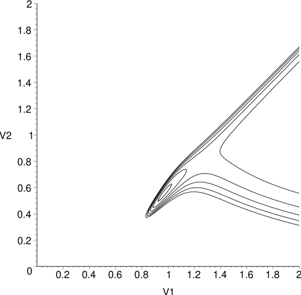
Figure 2: The contours show the value of the total potential including two gaugino condensates and the Casimir energy with the superpotential parameters given in Fig. 1. There is a minimum with zero potential and a saddle. The contour interval in this example is $\kappa_{4}^{-2}|W_{f}|^{2}$.

The example shown in Fig. 2 has a very large Casimir energy contribution. For smaller Casimir energies, Eq. (39) implies that the separation in the fifth dimension is similar in size to the Calabi-Yau radius and we have to consider carefully whether other Kaluza-Klein states contribute to the vacuum energy. The least massive Kaluza-Klein states have a mass $m_{CY}$ related to the first non-zero eigenvalue $\lambda_{1}$ of the second order perturbation operators on the Calabi-Yau space,

$$m_{CY}^{2}=\lambda_{1}v_{CY}^{-1/3}.$$ (40)

If the total vacuum energy vanishes, then Eq. (39) holds and using Eqs. (19-21) we have

$$l_{5}m_{CY}={2\sqrt{2}\over 3}\left({9C\over 2\pi}\right)^{1/5}\left({\tau-\mu\over\mu\tau\beta}\right)^{2/5}\alpha_{GUT}^{1/10}\,\lambda_{1}^{1/2}\approx 0.39C^{1/5}\lambda_{1}^{1/2}.$$ (41)

The massive Kaluza-Klein states can be neglected when $l_{5}m_{CY}\gg 1$. This can happen if $C$ is large or if the Calabi-Yau background has a relatively large first eigenvalue.

The values of the first eigenvalue of the scalar Laplacian on a Calabi-Yau space have been evaluated for specific examples using numerical methods by Braun et. al. Braun et al. (2008). The values range between around $20$ for a Fermat quintic to around $100$ for some more complicated cases. The larger values are already marginally consistent with a five-dimensional reduction unless $C$ happens to be very small (or indeed negative). It would be interesting to find out whether even larger values can be realised, especially for large values of the topological index $\beta$.

If the Kaluza-Klein modes contribute significantly to the vacuum energy, then the Casimir energy might still be able raise the minimum of the potential, but a more sophisticated calculation of the vacuum energy is required. Another possibility is that the warping is large, in which case a curved space casimir calculation is required.

III.3 Stabilisation with non-perturbative terms

If there are no high energy condensates on the visible brane, then we can replace the condensate on the visible brane with another non-perturbative effect. The usual candidate for this is a membrane which stretches between the two boundaries. The area of the membrane $\propto V_{1}-V_{2}$ and the type of contribution this gives to the superpotential is

$$W_{np}=ce^{-\tau(V_{1}-V_{2})}.$$ (42)

The total superpotential for the toy model is given by

$$W=be^{-\mu V_{2}}+ce^{-\tau(V_{1}-V_{2})}-w,$$ (43)

where $w=-W_{f}$ and $b$, $c$ are constants.

This time the parameters $b$, $c$ and $w$ given in terms of the values of $V_{1}$ and $V_{2}$ at the supersymmetric minimum are shown in figure 3. There are always supersymmetric minima in the parameter region indicated on the figure. The minimum potential is now given by

$$V_{\rm min}=-{27\over 32}\mu^{2}\Phi^{2}(V_{1}^{1/3}-V_{2}^{1/3})^{-2}\kappa_{4}^{-2}\alpha^{2}\epsilon^{2}\Lambda^{2}.$$ (44)

Figure 3: The contours show the value of the volume modulus $V_{2}$ at the supersymmetric minimum of the potential. The axes are the superpotential parameters $b$ and $c$ and values of $\tau$ range from $\mu/2$ to $2\mu$. In this case $c$ and $\tau$ parameterise the membrane contribution $W_{np}$. The spot marks the parameters used for Fig. 4. This plot uses the physical value of the volume modulus $V_{1}$ where $\mu V_{1}=5$.

The same procedure as before can now be used to determine whether the Casimir energy is able to cancel the negative gaugino induced potential. For small warping,

$$V_{\rm min}=-{729\over 128}\mu^{2}\Phi^{2}V_{1}^{-1}(V_{1}-V_{2})^{-3}\kappa_{4}^{-2}\alpha^{2}\epsilon^{2}\Lambda^{2}.$$ (45)

The five-dimensional Casimir energy (37) can cancel the negative gaugino induced potential when

$$(V_{1}-V_{2})^{3}={32C\over 81\mu^{2}}V_{1}^{-2}\alpha^{2}\kappa_{4}^{2}.$$ (46)

This can be arranged by choosing $b$, $c$ and $w$. The potential is shown in Fig. 4, and like in the previous case it has a single minimum and a single saddle point. The size of the extra dimension satisfies

$$l_{5}m_{CY}={4\sqrt{2}\over 9}\left({9C\over 4\pi\mu^{2}}\right)^{1/3}\alpha_{GUT}^{1/2}\,\lambda_{1}^{1/2}\approx 0.038C^{1/3}\lambda_{1}^{1/2}.$$ (47)

Either the first eigenvalue needs to be larger than in the previous case or we have to include the Kaluza-Klein modes.

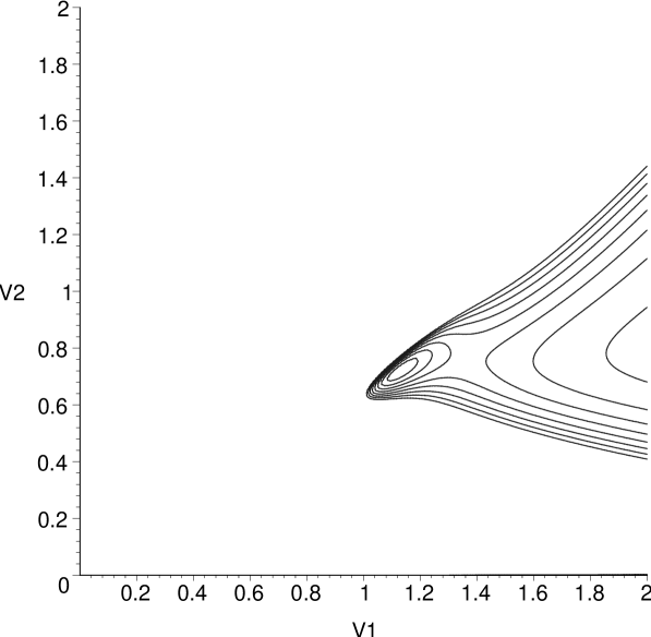
Figure 4: The contours show the value of the total potential including the supermembrane potential and the Casimir energy using the superpotential parameters given in Fig. 3 . There is a local minimum with zero potential and a saddle. The contour interval in this example is $0.01\kappa_{4}^{-2}|W_{f}|^{2}$.

The most general situation is one in which there are combinations of different condensate-like terms and non-perturbative terms in the superpotential. When the Calabi-Yau space has $h_{1,1}>1$ there are additional $(1,1)$ moduli which can all be fixed at the minimum of the potential Braun and Ovrut (2006). The general case has a potential similar to (38) at the minimum, and the balancing this against the Casimir energy gives a consistency condition which is more like Eq. (41) than Eq. (47).

IV Vacuum energy of the gravitino

After reduction from eleven to five dimensions, the theory contains a graviton multiplet and a scalar hypermultiplet. The hypermultiplet includes the Calabi-Yau volume field $V$. In the general case, there is also a collection of $h_{1,1}-1$ vector multiplets and a set of $h_{2,1}$ hypermultiplets. The quantum vacuum energy of the vector multiplets was evaluated in Ref. Moss and Norman (2004), and as expected there was a cancellation between the contributions from the bosonic and fermionic fields . In this section, we shall consider the graviton multiplet and include the gaugino condensate. We expect to see effects on the vacuum energy from the twisting of the gravitino boundary conditions and from changes in the mass of the gravitino. We shall only give results in the case where the warping of the fifth dimension is small, but even in this case we have to face some new technical issues.

IV.1 Twisted fermion boundary conditions

Majorana fermion fields in five dimensions have 8 components which can conveniently be placed into an 8-spinor $\psi$. The gamma-matrix representation which we use is

$$\hat{\Gamma}_{\mu}=\pmatrix{\gamma_{\mu}&0\cr 0&-\gamma_{\mu}\cr},\qquad\hat{\Gamma}_{5}=\pmatrix{\gamma_{5}&0\cr 0&-\gamma_{5}\cr},$$ (48)

where $\gamma_{\mu}$, $\mu=1\dots 4$ are the usual Dirac gamma-matrices. Following Ref. Flachi et al. (2001b), we start with identical chirality conditions on the spinor fields on the two flat boundary components,

$$\psi=\hat{\Gamma}_{5}\psi.$$ (49)

Twisted boundary conditions are obtained by applying a similarity transformation to the spinor representation at the hidden brane, so that the boundary condition there becomes

$$\psi=e^{i\theta\hat{\Gamma}/2}\hat{\Gamma}_{5}e^{-i\theta\hat{\Gamma}/2}\psi,$$ (50)

where $\theta$ is a real number and $\hat{\Gamma}$ anti-commutes with the other $\gamma$-matrices, for example

$$\hat{\Gamma}=\pmatrix{0&1\cr 1&0}.$$ (51)

The special case $\theta=\pi$ results in a fermion with opposite chirality on the two boundaries.

In the flat space limit, the Kaluza-Klein masses for the twisted fermion modes become $(n\pi\pm\theta/2)/l_{5}$, where $l_{5}$ is the separation of the two boundaries. The Casimir energy $V_{F}(\theta)$ for these modes is Flachi et al. (2001a, b)

$$V_{F}(\theta)=\pm{3\over 64\pi^{2}}l_{5}^{-4}\sum_{n=1}^{\infty}{\cos n\theta\over n^{5}},$$ (52)

where the plus sign is for ordinary fermions and the minus sign for ghosts.

In the case of a supermultiplet, the total Casimir energy is the sum of Fermionic and Bosonic contributions,

$$V_{T}=V_{F}(\theta)+V_{B}(\theta).$$ (53)

The total Casimir energy vanishes in the supersymmetric limit where $\theta=0$. If the bosonic modes are unaffected by the twist, then $V_{B}(\theta)=V_{B}(0)=-V_{F}(0)$ and the total Casimir energy in the 5-dimensional Einstein frame is given by

$$V_{T}=V_{F}(\theta)-V_{F}(0)=\mp{3\over 32\pi^{2}}l_{5}^{-4}\sum_{n=1}^{\infty}{\sin^{2}(n\theta/2)\over n^{5}}.$$ (54)

For small $\theta$,

$$V_{T}(\theta)\approx\mp{3\over 128\pi^{2}}\zeta(3)l_{5}^{-4}\theta^{2}.$$ (55)

where $\zeta$ is the Riemann zeta function. The upper sign is for ordinary fermions and the lower sign for ghosts.

IV.2 The gravitino contribution

We shall see now that the 11-dimensional gravitino in the lightest Calabi-Yau mode is equivalent to the twisted 5-dimensional fermion which was dealt with in the last section. The demonstration falls into two parts. The first part follows directly from the 11-dimensional boundary conditions and the second part of the process is to gauge away the condensate contribution to the fermion operators. The boundary conditions and fermion operators of the 11-dimensional theory are described in the appendix.

We take two flat boundary components separated in the $z=x^{5}$ direction labelled by the index $j=1$ for the visible brane (smaller $z$) and $j=2$ for the hidden brane (larger $z$). The 11-dimensional spinors are all in the lightest Calabi-Yau fermion mode which is the covariantly-constant Calabi-Yau spinor.

The boundary conditions on the tangential gravitino components are

$$\left(P_{\pm}\pm\epsilon\Gamma P_{\mp}\right)\lambda_{\mu}=0,$$ (56)

where $\Gamma$ was defined in Eq. (6). The upper signs are used for the visible brane, the lower for the hidden brane, and

$$P_{\pm}=\frac{1}{2}\left(1\pm\Gamma_{N}\right)=\frac{1}{2}\left(1-\Gamma_{5}\right).$$ (57)

When there is a gaugino condensate (24), then by considering $\Gamma^{2}$ it is possible to conclude that,

$$\Gamma={i\over 2}\Lambda_{j}V_{j}^{-1/2}\hat{\Gamma}$$ (58)

where $\hat{\Gamma}^{2}=1$ and $\{\hat{\Gamma},\Gamma_{\alpha}\}=0$ for $\alpha=1\dots 5$. This allows us to rewrite the boundary condition (56) on brane $j$ in the form

$$\lambda_{\mu}=e^{i\theta_{j}\hat{\Gamma}/2}\Gamma_{5}e^{-i\theta_{j}\hat{\Gamma}/2}\lambda_{\mu}$$ (59)

where

$$\theta_{j}=\mp 2\arctan\frac{1}{2}\epsilon\Lambda_{j}V_{j}^{-1/2}\approx\mp\epsilon\Lambda_{j}V_{j}^{-1/2},$$ (60)

for small $\epsilon\Lambda_{j}$. This is equivalent to the boundary condition Eq. (50) when written in 5-dimensional spinor form.

The gauge-ghost $\eta$ has the same boundary conditions as the tangential gravitino, but the gauge ghost $\nu$ and the Nielsen-Kallosh ghost swaps the classes $S_{+}$ and $S_{-}$ (see the appendix). For these

$$c=-e^{i\theta_{j}\hat{\Gamma}/2}\Gamma_{5}e^{-i\theta_{j}\hat{\Gamma}/2}c$$ (61)

where

$$\theta_{j}\approx\pm\epsilon\Lambda_{j}V_{j}^{-1/2}.$$ (62)

The normal component of the gravitino has the same value of $\theta_{j}$ as the tangential components. Note that we can use a similarity transformation to reduce the value of $\theta_{j}$ at the visible brane to zero, but before doing this we have to consider the fermion operators.

The fermion operators $D_{m}$ given in Eq. (74) depend on the background $G$ flux, which consists of the brane induced part $G_{0}$ and the condensate induced part $G_{g}$ (25). The condensate part will give a contribution to the fermion determinants. Fortunately, it is possible to gauge away the condensate terms from the operators using

$$D_{m}=e^{-i\Theta\hat{\Gamma}/2}\left(\Gamma^{I}D_{I}-\frac{\sqrt{2}}{96}m\Gamma^{IJKL}G^{0}_{IJKL}\right)e^{i\Theta\hat{\Gamma}/2}$$ (63)

where $\Theta$ is a function of $z$,

$$\Theta=-\frac{8}{5}m\epsilon\Lambda\Phi^{2}(V_{1}^{5/6}-V^{5/6}).$$ (64)

This transformation transfers the effect of the gaugino condensate terms to the boundary condition on the hidden brane, where

$$\Theta\approx-m\epsilon\Lambda V_{1}^{-1/2},$$ (65)

for small warping. We now combine (60) or (62) with the transformation (65) to get the total twist at the hidden brane

$$\theta=\epsilon\Lambda V_{1}^{-1/2}(\pm 1-m).$$ (66)

where the upper sign is for the gravitino (with $m=1$) and the gauge ghost $\eta$ (with $m=1/3$), whilst the lower sign is for the gauge ghost $\nu$ (with $m=1/3$) and the Nielsen-Kallosh ghost (with $m=-3$) . For small warping, the gravitino components are effectively untwisted, but the two gauge-ghost fermions and the Nielsen-Kallosh ghost survive as twisted fermions. The total contribution to the Casimir energy (55) based on (66) is

$$V_{T}={3\over 128\pi^{2}}\zeta(3)\left(\frac{20}{9}+4\right)l_{5}^{-4}V_{1}^{-1}\epsilon^{2}\Lambda^{2}.$$ (67)

In terms of the constant $C$,

$$V_{T}=Cl_{5}^{-4}V_{1}^{-1}\epsilon^{2}\Lambda^{2}.$$ (68)

where $C\approx 1.776\times 10^{-2}$ or $C^{1/5}\approx 0.45$. The cancellations have resulted in a small positive contribution to the vacuum energy. If the gravitino makes the only contribution to the Casimir energy, we could satisfy the consistency condition (41) only when the first eigenvalue on the Calabi-Yau space $\lambda_{1}\gg 32$. Alternatively, other multiplets may contribute to the Casimir energy and reduce the consistency bound on the first eigenvalue.

V conclusion

The aim of the present paper has been to show that, in principle, the Casimir energy can cancel other contributions to the the cosmological constant in reductions of heterotic $M$-theory. The Casimir energy arises from extra dimensions, where the fermion boundary conditions can break the supersymmetry. Since the boundary conditions and the moduli stabilisation potential can both be related to the scale of a gaugino condensate, cancellation of the cosmological constant requires the cancellation of two terms with similar scales, although the fine-tuning of a parameter in the superpotential is still required.

An explicit calculation of the Casimir energy for the gravitino revealed that the energy has the correct sign, and the size of the contribution was marginally consistent the parameter range for which the 5-dimensional calculation was valid. The validity of the approximation improves with the size of the first eigenvalue of the Laplacian on the Calabi-Yau space, and so examples of Calabi-Yau spaces with large first eigenvalues would be of interest. Two ways to improve the Casimir calculation itself would be to allow large warping of the metric in the fifth dimension and to extend the results to the full eleven dimensions. Some preliminary work has already been done with large warping Ahmed (2008), and on the casimir energy for manifolds with topology $R^{4}\times S^{1}/Z_{2}\times S^{2}$ Flachi et al. (2003).

The gravitino makes the largest contribution to the casimir energy because the gravitino boundary conditions are influenced directly by the condensate. However, other fields may receive smaller indirect effects, through changes in the background metric for example, and these can also contribute towards the Casimir energy. The first step towards calculating the contribution from these fields should be a full 5-dimensional reduction of the new version of heterotic $M$-theory, which has not yet been done. It should be possible to express the bulk fields of the reduced theory in terms of 5-dimensional supergravity multiplets, as in Ref. Lukas et al. (1999b), and the boundary conditions on these multiplets are currently under investigation.

Another avenue for further work would be extending the results of this paper to include the presence of 5-branes and anti-5-branes, which seem to be required for obtaining something approaching the standard model of particle physics at low energies Braun and Ovrut (2006). At present, the modifications to the boundary conditions required for 5-branes are not understood, but it seems likely that a 5-brane running parallel to the boundary branes will lead to two independent sets of twisted fermion boundary conditions on the boundary branes.

We turn finally to the prospects for heterotic $M$-theory cosmology. The potential for the volume moduli has a saddle point separating the local minimum from the large volume region with zero potential. If the potential barrier though the saddle point is sufficiently wide, an inflationary type of evolution from the saddle to the local minimum in the potential is possible. This case also allows an instanton representing the ‘ex nihilo’ creation of the universe at the saddle point Hawking and Moss (1982). By complete contrast, since the potential becomes positive and infinite when the brane separation shrinks to zero, it seems to also allow a colliding brane type of cosmological scenario Khoury et al. (2001). For this scenario, the vacuum energy would be tuned to be small at the saddle point, rather than at the minimum of the potential.

Appendix A The gravitino in 11-dimensions

In this appendix we shall give some details about gauge-fixing for the gravitino in eleven dimensions, and obtain the boundary conditions on the gravitino and ghost fields.

The 2-fermion gravitino Lagrangian ${\cal L}_{RS}$ is part of the supergravity action (1),

$${\cal L}_{RS}=-\bar{\Psi}_{I}\Gamma^{IJK}D_{J}\Psi_{K}-\frac{\sqrt{2}}{96}\left(\bar{\Psi}_{I}\Gamma^{IJKLMP}\Psi_{P}+12\bar{\Psi}^{J}\Gamma^{KL}\Psi^{M}\right)G_{JKLM}.$$ (69)

The action is invariant under the supersymmetry transformation

$$\delta\Psi_{I}=D_{I}\eta+{\sqrt{2}\over 288}\left(\Gamma_{I}\Gamma^{JKLM}-12\delta_{I}{}^{J}\Gamma^{KLM}\right)G_{JKLM}\eta.$$ (70)

We shall replace the supersymmetry invariance with a BRST invariance by introducing gauge fixing function

$$\Psi=\Gamma^{I}\Psi_{I},$$ (71)

and ghost fields. The general procedure is similar to the case of supergravity in four dimensions, and leads to three ghosts, a pair of gauge-fixing ghosts and the Nielsen-Kallosh ghost Nielsen (1978); Kallosh (1978). The 11-dimensional description below follows Freed and Moore Freed and Moore (2006) in general philosophy. Note that it is not known how to close the supersymmetry algebra off-shell in eleven dimensions, and so the BRST approach is not fully justified. We proceed under the assumption that the one-loop results are reliable nevertheless.

It is convenient to redefine the gravitino field first by introducing

$$\lambda_{I}=\Psi_{I}-\frac{1}{2}\Gamma_{I}\Psi.$$ (72)

The gravitino Lagrangian becomes

$${\cal L}_{RS}=-\bar{\lambda}^{I}D_{1}\lambda_{I}+\frac{9}{4}\bar{\Psi}D_{-3}\Psi-{\sqrt{2}\over 4}\bar{\lambda}^{I}\Gamma^{JK}\lambda^{L}G_{IJKL},$$ (73)

where

$$D_{m}=\Gamma^{I}D_{I}-{\sqrt{2}\over 96}m\Gamma^{IJKL}G_{IJKL}$$ (74)

The convenient choice of gauge-fixing term ${\cal L}_{GF}$ is the one which simplifies the total Lagrangian,

$${\cal L}_{GF}=-\frac{9}{4}\bar{\Psi}D_{-3}\Psi.$$ (75)

With this choice, the ghost action ${\cal L}_{GH}$ becomes

$${\cal L}_{GH}=-\bar{\nu}\delta\Psi-\bar{c}D_{-3}c,$$ (76)

where $\nu$ and $\mu$ are gauge ghosts and $c$ is the Nielsen-Kallosh ghost. BRST invariance requires

$$\delta\nu=-\frac{9}{2}D_{-3}\Psi$$ (77)

Using Eqs. (71) and (70) gives $\delta\Psi=D_{1/3}\eta$, and

$${\cal L}_{GH}=-\bar{\nu}D_{1/3}\eta-\bar{c}D_{-3}c.$$ (78)

The total action with Lagrangian ${\cal L}_{TOT}={\cal L}_{RS}+{\cal L}_{GF}+{\cal L}_{GH}$ is then invariant under the BRST transformations given by Eqs. (70) and (77), with all other BRST variations vanishing.

The boundary conditions on the tangential gravitino components and the supersymmetry parameter, given by Eq. (5), are fixed by the supersymmetry, but nothing has been determined so far about the boundary conditions on the normal component of the gravitino. Now we shall show that the boundary conditions on the ghost fields and the normal gravitino component $\lambda_{N}$ are uniquely determined by requiring them to be BRST invariant. (For an explanation of the relationship between BRST symmetry and boundary conditions, see Ref. Moss and Silva (1997)).

Consider one boundary component ${\cal M}_{j}$. Two sets of spinors $S_{\pm}$ can be defined by the action of the projection operators of Heterotic $M$-theory,

$$\psi\in S_{-} (P_{-}-\epsilon\Gamma P_{+})\psi=0\hbox{ on }{\cal M}_{j},$$ if (79)

$$\psi\in S_{+} (P_{+}+\epsilon\Gamma P_{-})\psi=0\hbox{ on }{\cal M}_{j}.$$ if (80)

According to (5), if there are no background supercurrents, the theory has

$$\Psi_{A},\ \eta\in S_{-}.$$ (81)

on the hidden brane. The operator $D_{m}$ maps from gauge ghosts in $S_{-}$ to gauge ghosts in $S_{+}$. Under BRST transformations $\delta\Psi=D_{1/3}\eta\in S_{+}$, therefore we conclude that $\Psi\in S_{+}$. The relationship between the ghost $c$ and $\Psi$ then implies

$$\Psi,\ c\in S_{+}.$$ (82)

The operator $D_{m}$ is self-adjoint on Majorana fermions, so that the BRST transformation (77) implies,

$$\nu\in S_{+}$$ (83)

For the boundary conditions on $\lambda_{I}$ we shall consider the case where $\Gamma$ anticommutes with $\Gamma_{I}$ (which is relevant for the gaugino condensate when $I=1\dots 5$), and then from (81) and (82),

$$\lambda_{A}\in S_{-}$$ (84)

The boundary conditions on $\lambda_{N}$ follow from Eq. (82),

$$(P_{+}+\epsilon\Gamma P_{-})(\Gamma^{A}\Psi_{A}+\Gamma^{N}\Psi_{N})=0.$$ (85)

This implies that

$$(P_{+}-\epsilon\Gamma P_{-})\lambda_{N}=0$$ (86)

and we call this set of spinors $\bar{S}_{-}$. This completes a consistent set of boundary conditions, but it would be interesting to extend these further to include the Yang-Mills fields and to understand their mathematical significance better.

References

- Horava and Witten (1996a) P. Horava and E. Witten, Nucl. Phys. B460, 506 (1996a), eprint hep-th/9510209.
- Horava and Witten (1996b) P. Horava and E. Witten, Nucl. Phys. B475, 94 (1996b), eprint hep-th/9603142.
- Witten (1996) E. Witten, Nucl. Phys. B471, 135 (1996), eprint hep-th/9602070.
- Banks and Dine (1996) T. Banks and M. Dine, Nucl. Phys. B479, 173 (1996), eprint hep-th/9605136.
- Moss (2003) I. G. Moss, Phys. Lett. B577, 71 (2003), eprint hep-th/0308159.
- Moss (2005) I. G. Moss, Nucl. Phys. B729, 179 (2005), eprint hep-th/0403106.
- Moss (2006) I. G. Moss, Phys. Lett. B637, 93 (2006), eprint hep-th/0508227.
- Moss (2008) I. G. Moss, JHEP 11, 067 (2008), eprint 0810.1662.
- Lukas et al. (1999a) A. Lukas, B. A. Ovrut, K. S. Stelle, and D. Waldram, Phys Rev D 59, 086001 (1999a).
- Lukas et al. (1999b) A. Lukas, B. A. Ovrut, K. S. Stelle, and D. Waldram, Nucl. Phys. B552, 246 (1999b), eprint hep-th/9806051.
- Kachru et al. (2003a) S. Kachru, M. B. Schulz, and S. Trivedi, JHEP 10, 007 (2003a), eprint hep-th/0201028.
- Kachru et al. (2003b) S. Kachru, R. Kallosh, A. Linde, and S. P. Trivedi, Phys. Rev. D68, 046005 (2003b), eprint hep-th/0301240.
- Buchbinder and Ovrut (2004) E. I. Buchbinder and B. A. Ovrut, Phys. Rev. D69, 086010 (2004), eprint hep-th/0310112.
- Braun and Ovrut (2006) V. Braun and B. A. Ovrut, JHEP 07, 035 (2006), eprint hep-th/0603088.
- Curio and Krause (2002) G. Curio and A. Krause, Nucl. Phys. B643, 131 (2002), eprint hep-th/0108220.
- Dine et al. (1985) M. Dine, R. Rohm, N. Seiberg, and E. Witten, Phys. Lett. B156, 55 (1985).
- Horava (1996) P. Horava, Phys. Rev. D54, 7561 (1996), eprint hep-th/9608019.
- Lukas et al. (1998) A. Lukas, B. A. Ovrut, and D. Waldram, Phys. Rev. D57, 7529 (1998), eprint hep-th/9711197.
- Gray et al. (2007) J. Gray, A. Lukas, and B. Ovrut, Phys. Rev. D76, 126012 (2007), eprint 0709.2914.
- Becker et al. (2004) M. Becker, G. Curio, and A. Krause, Nucl. Phys. B693, 223 (2004), eprint hep-th/0403027.
- Antoniadis and Quiros (1997) I. Antoniadis and M. Quiros, Nucl. Phys. B505, 109 (1997), eprint hep-th/9705037.
- Toms (2000) D. J. Toms, Phys. Lett. B484, 149 (2000).
- Garriga et al. (2001) J. Garriga, O. Pujolas, and T. Tanaka, Nucl. Phys. B605, 192 (2001), eprint hep-th/0004109.
- Garriga et al. (2003) J. Garriga, O. Pujolas, and T. Tanaka, Nucl. Phys. B655, 127 (2003), eprint hep-th/0111277.
- Flachi et al. (2003) A. Flachi, J. Garriga, O. Pujolas, and T. Tanaka, JHEP 08, 053 (2003), eprint hep-th/0302017.
- Fabinger and Horava (2000) M. Fabinger and P. Horava, Nucl. Phys. B580, 243 (2000), eprint hep-th/0002073.
- Flachi et al. (2001a) A. Flachi, I. G. Moss, and D. J. Toms, Phys. Lett. B518, 153 (2001a), eprint hep-th/0103138.
- Flachi et al. (2001b) A. Flachi, I. G. Moss, and D. J. Toms, Phys. Rev. D64, 105029 (2001b), eprint hep-th/0106076.
- Green et al. (1987) M. B. Green, J. H. Schwarz, and E. Witten, Superstring Theory. vol. 2: Loop amplitudes, anomalies and phenomenology (1987), Cambridge University press, UK. (Cambridge Monographs On Mathematical Physics).
- Luckock and Moss (1989) H. C. Luckock and I. G. Moss, Class Quantum Grav 6, 1993 (1989).
- Lukas et al. (1999c) A. Lukas, B. A. Ovrut, and D. Waldram, Nucl. Phys. B540, 230 (1999c), eprint hep-th/9801087.
- Ahmed and Moss (2008) N. Ahmed and I. G. Moss, JHEP 12, 108 (2008), eprint 0809.2244.
- Curio and Krause (2001) G. Curio and A. Krause, Nucl. Phys. B602, 172 (2001), eprint hep-th/0012152.
- Paccetti Correia et al. (2006) F. Paccetti Correia, M. G. Schmidt, and Z. Tavartkiladze, Nucl. Phys. B751, 222 (2006), eprint hep-th/0602173.
- Burgess et al. (1996) C. P. Burgess, J. P. Derendinger, F. Quevedo, and M. Quiros, Annals Phys. 250, 193 (1996), eprint hep-th/9505171.
- Braun et al. (2008) V. Braun, T. Brelidze, M. R. Douglas, and B. A. Ovrut, JHEP 07, 120 (2008), eprint 0805.3689.
- Moss and Norman (2004) I. G. Moss and J. P. Norman, JHEP 09, 020 (2004), eprint hep-th/0401181.
- Ahmed (2008) N. Ahmed, Brane worlds and low-energy heterotic -theory (2008), PhD thesis.
- Hawking and Moss (1982) S. W. Hawking and I. G. Moss, Phys. Lett. B110, 35 (1982).
- Khoury et al. (2001) J. Khoury, B. A. Ovrut, P. J. Steinhardt, and N. Turok, Phys. Rev. D64, 123522 (2001), eprint hep-th/0103239.
- Nielsen (1978) N. K. Nielsen, Nucl. Phys. B140, 499 (1978).
- Kallosh (1978) R. E. Kallosh, Nucl. Phys. B141, 141 (1978).
- Freed and Moore (2006) D. S. Freed and G. W. Moore, Commun. Math. Phys. 263, 89 (2006), eprint hep-th/0409135.
- Moss and Silva (1997) I. G. Moss and P. J. Silva, Phys. Rev. D55, 1072 (1997), eprint gr-qc/9610023.
- Lukic and Moore (2007) S. Lukic and G. W. Moore (2007), eprint hep-th/0702160.