Incompatibility of Rotation Curves with Gravitational Lensing for TeVeS

Abstract

We constrain the one-parameter ($\alpha$) class of TeVeS models by testing the theory against both rotation curve and strong gravitational lensing data on galactic scales, remaining fully relativistic in our formalism. The upshot of our analysis is that – at least in its simplest original form, which is the only one studied in the literature so far – TeVeS is ruled out, in the sense that the models cannot consistently fit simultaneously the two sets of data without including a significant dark matter component. It is also shown that the details of the underlying cosmological model are not relevant for our analysis, which pertains to galactic scales. The choice of the stellar Initial Mass Function – which affects the estimates of baryonic mass – is found not to change our conclusions.

I Introduction

With the availability of “precision” cosmological data, it has been possible to formulate and test the standard ($\Lambda$CDM) cosmological model to unprecedented accuracy, with the paradigm consistently proving itself to be highly successful at fitting observations teg06 . The model is based on two key components: a framework of classical general relativity acting on a homogeneous Friedman-Lemaître-Robertson-Walker metric with cosmological constant, $\Lambda~{}>~{}0$, and the presence of Cold Dark Matter (CDM). There have been, however, other proposals for models that lie outside the $\Lambda$CDM framework. Such models come from those who see the as yet undetected status of dark matter and the lack of a fundamental theory for the cosmological constant as impetus for looking into alternative theories. In particular, Milgrom milgrom put forward the MOdified Newtonian Dynamics (MOND) to explain the flat rotation curves of galaxies without invoking dark matter. Constructed to give flat rotation curves below an acceleration scale, $a_{0}\approx 1.2\times 10^{-10}{\rm m}/{\rm s}^{2}$, set by galactic rotation data, MOND modifies the standard Newtonian relation between the gravitational potential and the acceleration to $f(|{\vec{a}}|/a_{0}){\vec{a}}=-{\vec{\nabla}}\Phi_{\rm N}$, where $\Phi_{\rm N}$ is the Newtonian gravitational field. The function $f(x)$ is positive, smooth, and monotonic; it controls the interpolation between the two gravitational regimes above and below the acceleration scale. When $f(x)$ equals unity, the usual Newtonian dynamics holds, while when $f(x)$ approximately equals its argument, $f(x)\simeq x$, the deep MONDian regime applies.

MOND has proven itself to be very successful at fitting galactic rotation curves, but it has been less so when applied to galaxy clusters. A relativistic field theory counterpart to MOND has also been expounded bek ; sand , involving the inclusion of a TEnsor, VEctor and Scalar field (TeVeS). Since it has been constructed to reproduce the same modification to gravity as MOND in its low acceleration non-relativistic regime, TeVeS has not been tested using rotation curves; it has been applied to areas such as the cosmic microwave background sko06 and gravitational lensing, where the relativistic aspects of the theory could be fully exploited in a way unachievable by MOND. Most of the work on TeVeS and lensing has remained non-relativistic zhao06 ; Feix ; Feix2 , by simply reducing the theory to that approximately replicated through the addition of a scalar-field potential to the Newtonian potential. However, recent work msy has conducted a fully relativistic lensing analysis of TeVeS and applied the results to a sample of six lenses from the CASTLES survey. In order to ascertain the validity of the TeVeS/MOND claim of explaining observations without the inclusion of dark matter, the stellar content of these galaxies, determined by means of a non-parametric model-independent method, was compared to the mass predicted from lensing in the context of the TeVeS model. A discrepancy here would be indicative of a shortcoming of the theory in its fundamental claim. As the precise results of the comparison of these masses depended significantly on the exact form of the MOND $f(x)$ function, and its TeVeS equivalent $\mu(y)$, a parametrised range of these functions was considered. The analysis showed msy that the parametrisation commonly used for MOND and TeVeS requires significant quantities of dark matter, with the dependence increasing as the parametrisation moved to the functions which best fit rotation curves. These results suggest that a harmonisation between fitting both rotation curves and lensing may not be possible in these modified gravity theories.

The purpose of the present work is to fully examine the efficacy of TeVeS, using the two distinct approaches of rotation curves and lensing data in order to examine the validity of the implied deficiency found in the theory msy . Using the two methods and sets of data, in a fully relativistic way, we independently constrain the degeneracy that exists within the theory regarding the precise form of the $\mu(y)$ function. In this way we can check whether there is any single form of the theory which can fit and describe both rotation curves and lensing data.

The structure of the article is the following: In Section II, we describe the relevant formalism, and solving the appropriate classical equations for the metric in TeVeS. We then use this metric to find the modified equations for the deflection of light and circular rotation. In Section III we analyse rotation curve data for a selection of both High (HSB) and Low (LSB) Surface Brightness galaxies. In Section IV we analyse gravitational lensing for the constraints imposed by the rotation curves. We also find the parameter which fits best the lensing data, and examine how this fits with rotation curves. We round up with an analysis of the results, and present our conclusions and outlook in Section V.

II The TeVeS Model

In this section we shall review the relevant formalism, leading to the TeVeS dynamical equations, which are used when computing the deflection angle and other quantities to be used in our fitting procedure. We shall be brief in our analysis. For details we refer the reader to reviews and relevant previous work bek ; giannios ; msy ; sko09 . TeVeS bek is a bi-metric model in which matter and radiation do not feel the Einstein metric, $g_{\alpha\beta}$, that appears in the canonical kinetic term of the (effective) action, but a modified “physical” metric, ${\tilde{g}}_{\alpha\beta}$, related to the Einstein metric by

$$\tilde{g}_{\alpha\beta}=e^{-2\phi}g_{\alpha\beta}-U_{\alpha}U_{\beta}(e^{2\phi}-e^{-2\phi})~{},$$ (1)

where $U_{\mu},~{}\phi$ denote the TeVeS vector and scalar field, respectively. The TeVeS action reads

$$S= \int{\rm d}^{4}x\ \left[\frac{1}{16\pi G}\left(R-2\Lambda\right)-\frac{1}{2}\{\sigma^{2}\left(g^{\mu\nu}-U^{\mu}U^{\nu}\right)\phi_{,\alpha}\phi_{,\beta}+\frac{1}{2}Gl^{-2}\sigma^{4}F(kG\sigma^{2})\}\right.$$ (2)

$$\ \ \ \ \ \ \ \ \ \ \left.-\frac{1}{32\pi G}\left\{K{\cal F}^{\alpha\beta}{\cal F}_{\alpha\beta}-2\lambda\left(U_{\mu}U^{\mu}+1\right)\right\}\right](-g)^{1/2}+{\cal L}(\tilde{g}_{\mu\nu},f^{\alpha},f^{\alpha}_{|\mu},...)(-\tilde{g})^{1/2},$$

where $k,~{}K$ are the coupling constants for the scalar, vector field, respectively; $\ell$ is a free scale length related to $a_{0}$ (c.f below); $\sigma$ is an additional non-dynamical scalar field; ${\cal F}_{\mu\nu}\equiv U_{\mu,\nu}-U_{\nu,\mu}$; $\lambda$ is a Lagrange multiplier implementing the constraint $g^{\alpha\beta}U_{\alpha}U_{\beta}=-1$, which is completely fixed by variation of the action; the function $F(kG\sigma)$ is chosen to give the correct non-relativistic MONDian limit, with $G$ related to the Newtonian gravitational constant, $G_{\rm N}$, by $G=G_{\rm N}/[1+K/2+k/(4\pi)-2\phi_{\rm c}]$, where $\phi_{\rm c}$ is the present day cosmological value of the scalar field. Covariant derivatives denoted by $|$ are taken with respect to $\tilde{g}_{\mu\nu}$ and indices are raised/lowered using the metric $g_{\mu\nu}$.

The modified equations of motion can be calculated from the Lagrangian. For the modified Einstein equation we have bek ; giannios

$$G_{\alpha\beta}+g_{\alpha\beta}\Lambda=8\pi G\left[\tilde{T}_{\alpha\beta}+(1-e^{-4\phi})U^{\mu}\tilde{T}_{\mu(\alpha}U_{\beta)}+\tau_{\alpha\beta}\right]+~{}\Theta_{\alpha\beta}~{},$$ (3)

where

$$\tau_{\alpha\beta} \equiv \sigma^{2}[\phi_{,\alpha}\phi_{,\beta}-\frac{1}{2}g^{\mu\nu}\phi_{,\mu}\phi_{,\nu}g_{\alpha\beta}-U^{\mu}\phi_{,\mu}(U_{(\alpha}\phi_{,\beta)}-\frac{1}{2}U^{\nu}\phi_{,\nu}g_{\alpha\beta})]-\frac{G\sigma^{4}}{4l^{2}}F(kG\sigma^{2})g_{\alpha\beta}~{},$$

$$\Theta_{\alpha\beta} \equiv K(g^{\mu\nu}U_{[\mu,\alpha]}U_{[\nu,\beta]}-\frac{1}{4}g^{\sigma\tau}g^{\mu\nu}U_{[\sigma,\mu]}U_{[\tau,\nu]}g_{\alpha\beta})-\lambda U_{\alpha}U_{\beta}~{}.$$ (4)

For the vector field we obtain

$$8\pi G(1-e^{-4\phi})g^{\alpha\mu}U^{\beta}\tilde{T}_{\mu\beta}=K{U^{[\alpha;\beta]}}_{;\beta}+\lambda U^{\alpha}+8\pi G\sigma^{2}U^{\beta}\phi_{,\beta}g^{\alpha\gamma}\phi_{,\gamma}~{},$$ (5)

and similarly for the scalar field, namely

$$[\mu(y)(g^{\alpha\beta}-U^{\alpha}U^{\beta})\phi_{,\alpha}]_{;\beta}=kG[g^{\alpha\beta}+(1+e^{-4\phi})U^{\alpha}U^{\beta}]\tilde{T}_{\alpha\beta}~{},$$ (6)

with $\mu(y)$ defined by:

$$\mu(y) = kG\sigma^{2}~{},$$

$$y = -\mu F(\mu)-\frac{1}{2}\mu^{2}\frac{{\rm d}F(\mu)}{{\rm d}\mu}~{},$$

$$\quad y = kl^{2}(g^{\mu\nu}-U^{\mu}U^{\nu})\phi_{,\mu}\phi_{,\nu}~{}.$$ (7)

Motivated by the homogeneity and isotropy of the Universe, observed to date, we assume a spherically symmetric metric

$$g_{\alpha\beta}{\rm d}x^{\alpha}{\rm d}x^{\beta}=-e^{\nu}{\rm d}t^{2}+e^{\zeta}({\rm d}r^{2}+r^{2}{\rm d}\theta^{2}+r^{2}\sin^{2}\theta{\rm d}\varphi^{2})~{},$$ (8)

where $\nu$ and $\zeta$ are both functions of $r$. The physical metric can be written likewise, namely

$$\tilde{g}_{\alpha\beta}{\rm d}x^{\alpha}{\rm d}x^{\beta}=-e^{\tilde{\nu}}{\rm d}t^{2}+e^{\tilde{\zeta}}({\rm d}r^{2}+r^{2}{\rm d}\theta^{2}+r^{2}\sin^{2}\theta{\rm d}\varphi^{2})~{},$$ (9)

with the quantities $\tilde{\nu}$ and $\tilde{\zeta}$ related to $\nu$ and $\zeta$ by

$$\tilde{\nu}=\nu+2\phi~{}~{};~{}~{}\tilde{\zeta}=\zeta-2\phi~{}.$$ (10)

Isotropy makes the scalar field depending only on $r$, namely $\phi=\phi(r)$. We approximate matter as an ideal pressure-less fluid, $\tilde{T}_{\alpha\beta}=\tilde{\rho}\tilde{u}_{\alpha}\tilde{u}_{\beta}$. By assuming that the time-like vector field has only one non-zero temporal component, the normalisation condition imposed by the Lagrange multiplier restricts the vector field to be

$$U^{\alpha}=(e^{-\nu/2},0,0,0)~{}.$$ (11)

Considering the quasi-static case, we can take the four-velocity of the fluid, $\tilde{u}_{\alpha}$, to be collinear with $U^{\alpha}$, and then normalise it with respect to the physical metric, $\tilde{g}_{\alpha\beta}$, so that $\tilde{u}_{\alpha}=e^{\phi}U_{\alpha}$, leading to

$$\tilde{T}_{\alpha\beta}=\tilde{\rho}e^{2\phi}U_{\alpha}U_{\beta}~{}.$$ (12)

Thus, the scalar field equation, Eq.(6), along with the isotropy constraint, leads to

$$\frac{e^{-\frac{(\nu+3\zeta)}{2}}}{r^{2}}\left[r^{2}\phi^{\prime}e^{\frac{(\nu+\zeta)}{2}}\mu(y)\right]^{\prime}=kGe^{-2\phi}\tilde{\rho}~{},$$ (13)

where a prime denotes derivative with respect to $r$. Upon integration, we obtain

$$\phi^{\prime}=\frac{kGm_{\rm s}(<r)}{4\pi r^{2}\mu(y)}e^{-(\nu+\zeta)/2}~{},$$ (14)

where a scalar mass has been defined as

$$m_{\rm s}(<r)=4\pi\int^{r}_{0}\tilde{\rho}e^{\frac{\nu}{2}+\frac{3\zeta}{2}-2\phi}r^{2}{\rm d}r~{}.$$

As shown in Ref. bek , the scalar mass can, to a good approximation, be equivalent to the “proper” mass contained in the same volume. Moreover, the Lagrange multiplier appearing in the vector field, Eq.(11), can be totally determined by the vector equation, Eq.(5), namely

$$\lambda=8\pi G(e^{-2\phi}-e^{2\phi})\tilde{\rho}-Ke^{-\zeta}\left(\frac{\nu^{\prime\prime}}{2}+\frac{\nu^{\prime}\zeta^{\prime}}{4}+\frac{\nu^{\prime}}{r}\right)~{}.$$ (15)

Solving the modified Einstein equations, Eq. (3), for $\tilde{\nu}$ and $\tilde{\zeta}$ we find for the $(tt)$ and $(\theta\theta)$ components of the stress tensor

$$\tau_{tt} = \frac{kGm_{\rm s}(<r)^{2}}{32\pi^{2}\mu(y)}\frac{e^{-2\zeta}}{r^{4}}+\frac{\mu^{2}(y)}{4Gl^{2}k^{2}}F(\mu)e^{\nu}~{},$$

$$\tau_{\theta\theta} = -\frac{kGm_{\rm s}(<r)^{2}}{32\pi^{2}\mu(y)}\frac{e^{-(\zeta+\nu)}}{r^{2}}-\frac{\mu^{2}(y)}{4Gl^{2}k^{2}}F(\mu)r^{2}e^{\zeta}~{},$$

$$\Theta_{tt} = Ke^{\nu-\zeta}\left(\frac{(\nu^{\prime})^{2}}{8}+\frac{\nu^{\prime\prime}}{2}+\frac{\nu^{\prime}\zeta^{\prime}}{4}+\frac{\nu^{\prime}}{r}\right)-8\pi G\tilde{\rho}(e^{-2\phi}-e^{2\phi})e^{\nu}~{},$$

$$\Theta_{\theta\theta} = \frac{K}{8}(r\nu^{\prime})^{2}~{}.$$ (17)

Moreover, the Einstein tensor components are:

$$G_{tt} = -e^{\nu-\zeta}(\zeta^{\prime\prime}+\frac{(\zeta^{\prime})^{2}}{4}+\frac{2\zeta^{\prime}}{r})~{},$$

$$G_{\theta\theta} = \frac{r(\nu^{\prime}+\zeta^{\prime})}{2}+\frac{r^{2}(\nu^{\prime})^{2}}{4}+\frac{r^{2}(\zeta^{\prime\prime}+\nu^{\prime\prime})}{2}~{}.$$ (18)

We thus arrive at the following system of differential equations:

$$\zeta^{\prime\prime}+\frac{(\zeta^{\prime})^{2}}{4}+\frac{2\zeta^{\prime}}{r}+e^{\zeta}\Lambda = -\frac{kG^{2}m_{\rm s}^{2}}{4\pi\mu(y)}\frac{e^{-(\nu+\zeta)}}{r^{4}}-\frac{2\pi\mu^{2}(y)}{l^{2}k^{2}}F(\mu)e^{\zeta}$$

$$-K\left[\frac{(\nu^{\prime})^{2}}{8}+\frac{\nu^{\prime\prime}}{2}+\frac{\nu^{\prime}\zeta^{\prime}}{4}+\frac{\nu^{\prime}}{r}\right]-8\pi G\tilde{\rho}e^{\zeta-2\phi}~{},$$

$$\frac{(\nu^{\prime}+\zeta^{\prime})}{2r}+\frac{(\nu^{\prime})^{2}}{4}+\frac{\zeta^{\prime\prime}+\nu^{\prime\prime}}{2}+e^{\zeta}\Lambda = -\frac{kG^{2}m_{\rm s}^{2}}{4\pi\mu(y)}\frac{e^{-(\nu+\zeta)}}{r^{4}}-\frac{2\pi\mu^{2}(y)}{l^{2}k^{2}}F(\mu)e^{\zeta}+\frac{K}{8}\nu^{\prime 2}.$$ (19)

We analyse two distinct systems: lensing galaxies and galactic rotation curves. For the former, we model the system with the spherically symmetric mass profile hern :

$$M(<\hat{r})=\frac{M\hat{r}^{2}}{(\hat{r}+r_{\rm h})^{2}}~{},$$ (20)

where $\hat{r}=e^{\tilde{\zeta}/2}r$ is the Schwarzschild radial coordinate, $r_{\rm h}$ is the core radius scale, related to the projected two-dimensional half mass radius, $R_{\rm e}$, by $R_{\rm e}=1.8153r_{\rm h}$ fsw05 , and $M$ is the total mass of the galaxy. The mass, Eq. (20), specifies the density function ${\tilde{\rho}}$, and, as we mentioned previously, it is assumed approximately equal bek to the scalar mass $m_{\rm s}(<r)$.

For the galactic rotation curves, we use a different spherically symmetric mass profile, as outlined in Ref. mof , given in Schwarzschild radial coordinates by

$$M(<\hat{r})=M\left(\frac{\hat{r}}{r_{\rm c}+\hat{r}}\right)^{3\beta}~{},$$ (21)

where $\beta=1$ for HSB galaxies and $\beta=2$ for LSB galaxies; $r_{\rm c}$ is the core radius and $M$ is the total mass of the galaxy. We remark at this point that, when converting to the physical coordinates, a factor $e^{\tilde{\zeta}+2\phi}$ appears as the coefficient of the cosmological constant $\Lambda$.

In order solve the equations analytically, we have used the following approximation bek :

$$e^{2\phi}\simeq e^{2\phi_{\rm c}}\left[1-\frac{kGm_{\rm s}(<r)}{2\pi r}+\frac{k^{2}G^{2}m_{\rm s}^{2}(<r)}{8\pi^{2}r^{2}}+O(r^{-3})\right]~{}.$$ (22)

The precise form of the modification to gravity given in TeVeS is largely controlled by the $\mu(y)$ function, however, since the theory is not motivated from a microscopic theory, there exists a large amount of freedom in choosing the form of this function. In Ref. bek a toy-model function was suggested, namely

$$y=\frac{3}{4}\frac{\mu^{2}(\mu-2)^{2}}{1-\mu}~{}.$$ (23)

However, it was noted in Refs. mu1 and mu2 that when this function is converted to its MONDian equivalent, it fits rotation curve data worse than the standard MONDian “simple” form

$$f(x)=\frac{x}{\sqrt{1+x^{2}}}~{}.$$ (24)

In order to improve on this point, the authors of Ref. mu3 suggested the following function

$$f(x)=\frac{2x}{1+x+\sqrt{(1-x)^{2}+4x}}~{},$$ (25)

which fits better the rotation curve data in the MONDian framework.

In addition, they provided parametrised functions $f(x)$ and $\mu(y)$ which interpolate between the toy function, Eq. (23), and the “simple” function, Eq. (24), in both MOND and TeVeS frameworks, over the parameter range $0<\alpha\leq 1$:

$$f(x)=\frac{2x}{1+(2-\alpha)x+\sqrt{(1-\alpha x)^{2}+4x}}~{};\quad\mu(y)=\frac{\sqrt{\frac{y}{3}}}{1-\frac{2\pi\alpha}{k}\sqrt{\frac{y}{3}}}~{};~{}0<\alpha\leq 1~{}.$$ (26)

Note that, for $\alpha=0$, the function $\mu(y)$ does not coincide with the the toy function, Eq. (23), but rather approximates the function in the high and intermediate gravity regimes. However, this approximation is valid for our present analysis.

In fact, for our purposes, we find it convenient to use an explicit parametrisation of $\mu$ in terms of the scalar mass $m_{s}$, which is approximated by the mass profiles given directly by the data. To this end, we use Eq. (14) and the definition of $y$, Eq. (7), as well as the scalar equation of motion, Eq. (6), to write the parametric function $\mu(y)$ in Eq. (26) as:

$$\mu=\frac{2\pi\alpha j}{\sqrt{3}k}+\frac{2\pi}{k}\left(\frac{\alpha^{2}j^{2}}{3}+\frac{k^{2}j}{4\sqrt{3}\pi^{2}}\right)^{1/2}~{},\quad{\rm where}\ ~{}j(r)=\left(\frac{k^{3/2}\,lG}{4\pi}\right)\frac{m_{s}(<r)e^{-\tilde{\nu}/2-\tilde{\zeta}-\phi}}{r^{2}}~{}.$$ (27)

The corresponding $F$ function is then given by (c.f. Eq. (7)):

$$F(\mu)=\frac{6k^{3}}{(4\pi\alpha)^{3}\mu^{2}}\left[\ln\left(\frac{4\pi\alpha\mu}{k}+1\right)^{2}+\frac{1}{1+\frac{4\pi\alpha\mu}{k}}-\frac{4\pi\alpha\mu}{k}\right]~{}.$$ (28)

When $\alpha=0$, the function $F(\mu)$ becomes singular. Since the $\alpha=0$ case is supposed to give a very close approximation of the toy model function, we use for $\alpha=0$ the explicit expression for $F(\mu$) given in Ref. bek , which does not become singular. With all the various components given above, we are able to numerically solve the system of differential equations to find the functions $\tilde{\zeta}$, $\tilde{\nu}$, which specify the metric for our choice of the $\mu(y)$ function.

III Fitting Rotation Curves in TeVeS

In our metric system, Eq. (9), the equation for circular orbital velocity in TeVeS reads:

$$V_{\rm clr}=r\frac{{\rm d}\phi}{{\rm d}t}=\left(\frac{\tilde{\nu}^{\prime}r}{2+r\tilde{\zeta^{\prime}}}\right)^{1/2}~{}.$$ (29)

In order to perform a fitting analysis to rotation curve data there are two free fitting parameters: $r_{\rm c}$, which is the core radius of the galaxy, and $\alpha$, the parameter appearing in the TeVeS $\mu(y)$ function. For a particular choice of these parameters, we can predict the expected rotational velocity at certain radii and this is compared against data. Moreover, the constants in the TeVeS action, Eq. (2), are taken to be

$$k = 0.01~{};\quad K=0.01~{};\quad\ell=\sqrt{k\tilde{b}}/(4\pi\Xi a_{0})~{};$$

$$\phi_{\rm c} = 0.001~{};\quad\Xi=1+K/2-2\phi_{\rm c}~{}.$$ (30)

The values of $K$ and $k$ are constrained bek from solar system tests on gravity to be $\lesssim 0.1$, and by rotation curves to be $\gtrsim 0.001$. The scale $\ell$ is related to the MONDian acceleration scale, $a_{0}$ and $\tilde{b}$. The latter quantity is found by taking the limit of the function $y(\mu)$ when $\mu<<1$, which then takes the form $y(\mu)\approx\tilde{b}\mu$, so for the class of $\mu$ functions considered here, we set $\tilde{b}=3$. Finally we note that, for $\phi_{\rm c}$, the present day value of scalar field at cosmological scales, there are no tight constraints on its exact value, with an approximate upper bound coming from cosmological data.

With these constants so defined, we are able to numerically solve the equations and perform a fitting analysis for the galactic rotation curves. A standard likelihood analysis is used to determine the best fit parameters. Using $\chi^{2}$-statistics, the likelihood probability distribution function for the value of $\alpha$ using data from the $i^{th}$ galaxy is defined as

$$L_{i}(\alpha)=e^{-\frac{1}{2}[\chi_{i}^{2}(\alpha)-\chi^{2}_{i,{\rm min}}]}~{}.$$ (31)

The combined likelihood function for all the galaxies is therefore defined as:

$$L_{{\rm tot}}(\alpha)=L_{1}(\alpha)\times L_{2}(\alpha)\times L_{3}(\alpha)\times\cdots,$$ (32)

where the subscript on $L$ denotes the galaxy. The peak of the total likelihood represents the most likely value of $\alpha$, and the cumulative distribution is used to determine the 90% confidence level (i.e. comparing the 5- and 95-percentile of the distribution). The constraint on $\alpha$ from this analysis is then used to determine lensing masses, as shown below.

In order to find the minimum value of $\chi^{2}$ by numerically varying the free parameters, an adaptive grid method was implemented to give a value of $\chi^{2}$ accurate up to 2 decimal places. The sample of galaxies we chose to examine were taken from Refs. ver1 ; ver2 which explored the Tully-Fisher relation in galaxies belonging to the Ursa Major cluster. Only those rotation curves were examined for which there exist at least five data points and the inner part of the velocity distribution is available, i.e. we excluded those galaxies for which the data only recorded the velocity in the flat part of the rotation curve and missed the inner sections. This gave us a sample of 6 galaxies, 2 LSB (NGC 3972, NGC 4085) and 4 HSB (UGC 6399, UGC 6917, UGC 6923, UGC 7089). The photometric details of the galaxies are given in Table I.

Galaxy	$B-R$	$R-I$	$I-K$	MK	Mgas	Mst(Ch)	Mst(Salp)	MN
	Vegamag				$\times 10^{8}$M⊙			$\times 10^{10}$M⊙
NGC 3972	$0.97$	$0.43$	$1.60$	$-22.08$	$18.07$	$57.15$	$80.17$	$3.77$
NGC 4085	$0.99$	$0.46$	$1.70$	$-22.27$	$15.89$	$72.09$	$100.93$	$2.75$
UGC 6399	$0.88$	$0.33$	$1.56$	$-20.33$	$11.43$	$11.30$	$15.85$	$1.46$
UGC 6917	$0.86$	$0.35$	$1.26$	$-21.10$	$28.52$	$27.61$	$38.37$	$3.10$
UGC 6923	$0.83$	$0.53$	$1.16$	$-20.36$	$11.65$	$13.96$	$19.41$	$0.84$
UGC 7089	$0.85$	$0.30$	$1.04$	$-20.30$	$18.51$	$13.77$	$19.14$	$1.37$

Table 1: Photometric and baryonic mass data for the galaxies in our sample. The photometric data are corrected for internal extinction and are taken from from Table 2 of Ref. ver1 . $M_{{\rm gas}}$ is the gas mass from 21 cm fluxes corrected to include Helium, $M_{{\rm st}}$ is the calculated mass of the stellar content (given for both choices of the Initial Mass Function). M_N gives the Newtonian estimate for the total mass, by using the maximum observed radial position and the maximum rotation velocity: M${}_{\rm N}=v_{\rm MAX}^{2}R/G$.

The photometric details given in Table I are used to calculate the total baryonic content of the galaxies, fixing the mass parameter for TeVeS as M${}_{\rm gas}+$M_st. For the gas mass, we assume an infinitely thin disk and we use the observed 21 cm line fluxes (listed in Ref. ver1 ), using the standard translation between 21 cm flux and neutral hydrogen mass (see, e.g. Ref. mof ). A correction factor of 4/3 is necessary to take proper account of the presence of Helium in the gas phase.

For the stellar content of the galaxies it is important to choose realistic populations. Population synthesis models (e.g. Ref. bc03 ) combine our knowledge of stellar evolution with libraries of stellar spectra to obtain simple stellar populations (SSPs), which correspond to a family of stars all formed at the same time, with the same metallicity. Although SSPs can be used to describe the spectral energy distribution of globular clusters – which form over very short times compared to stellar evolution timescales – a galaxy has a more complex distribution of stellar ages. We follow here the same approach as in Ref. fsw05 , and run a grid of models with an exponentially decaying star formation history. These models replace the single age of a SSP by a linear superposition of SSPs according to an exponentially decaying function of time. Hence, a model is described by the following three parameters: (i) the epoch when the galaxy is born (chosen between redshifts z${}_{\rm F}=1$ and $10$), (ii) the timescale of the exponential (between $\log\tau$(Gyr)$=-1$ and $+1$) and (iii) the metallicity (between 1/30th and twice the solar abundance). Our “basis” SSP models are taken from Ref. cb07 ). We run a grid of $32\times 32\times 32$ models with a uniform distribution of the three parameters that describe the star formation history. For each choice, the models give a spectral energy distribution which is folded with the response function of the standard filters $B$, $R$, $I$ and $K$, which extend over a wide spectral range, from optical blue light ($\lambda\sim 0.4\mu$m) to near infrared ($\lambda\sim 2.2\mu$m). Our photometric system is referenced with respect to Vega. The resulting colours $B-R$, $R-I$ and $I-K$ are compared with the observations, defining a likelihood which is used to determine the stellar masses by comparing the best fit absolute magnitude in the near infrared band ($K$, $\lambda\sim 2.2\mu$m). At longer wavelengths, stellar mass estimates are more robust, since they minimise the attenuation from dust and the flux mostly originates from intermediate/low mass stars, which dominate the stellar mass budget.

In addition to age and metallicity, the stellar mass of a population depends sensitively on the mass distribution of stars at birth, i.e. the Initial Mass Function (IMF). It is generally assumed that the IMF is universal, although its shape at the low mass end is uncertain given how little low-mass stars contribute to the total luminosity of a population. In this paper we consider both the Chabrier IMF chab03 and the simple power law of Salpeter salp . Both IMFs roughly agree at the massive end – where observations can set significant constraints – however, at the low mass end, the Salpeter IMF simply extrapolates the distribution as a power law. Recent dynamical and lensing studies (see, e.g. Ref. cap ; FSans ) suggest that the Salpeter IMF gives unrealistically high stellar masses, and functions such as the Chabrier IMF – which replace the power law by a log-normal distribution at low masses– are favoured. However, given that all those analyses were based on a “standard” General Relativity (GR) / Newtonian theory, we present in this paper both choices of IMF (see, also Ref. sand08 ).

The total baryonic content is the sum of the stellar and the gas mass. Within the TeVeS framework, we assume that the baryonic masses are the total masses of galaxies and we combine them with the observed rotation curves to constrain the $\alpha$ parameter that characterises TeVeS. The values of the likelihood probability distribution function fits are plotted against the value of the $\alpha$ parameter. The results are given in Fig. 1 as a two-dimensional (2D) map with $\alpha$ vs. core radius. The contours are shown at the 75%, 90% and 95% confidence level for the Chabrier (red) and the Salpeter (blue) IMF. We also show the marginalised 1D likelihood function with respect to $\alpha$ in Fig. 2, with the results for the Chabrier and the Salpeter IMF given as a solid and dashed line, respectively. The values for the lowest $\chi^{2}$ and the corresponding values of $\alpha$ are given in Table II, where it can be seen that each of the galaxies analysed here gives a reasonable fit to the data once the $\chi^{2}$ is minimised. The results show that the best fit values for the $\alpha$ parameter are in the range $\sim(5-10)$.

		Salpeter			Chabrier
Galaxy	dof	$\alpha$	$\chi^{2}_{r}$	$\chi^{2}_{r}(\alpha=0)$	$\alpha$	$\chi^{2}_{r}$	$\chi^{2}_{r}(\alpha=0)$
NGC 3972	$9$	$\rightarrow\infty$	$5.20$	$38.05$	$11.19$	$2.47$	$28.13$
NGC 4085	$5$	$\rightarrow\infty$	$3.25$	$21.33$	$\rightarrow\infty$	$0.63$	$15.45$
UGC 6399	$7$	$6.73$	$1.06$	$3.51$	$5.32$	$1.15$	$2.81$
UGC 6917	$9$	$13.84$	$1.12$	$20.91$	$9.56$	$1.23$	$17.59$
UGC 6923	$4$	$11.66$	$1.31$	$4.8$	$12.14$	$1.30$	$4.87$
UGC 7089	$10$	$8.53$	$0.58$	$2.71$	$7.12$	$0.6$	$2.26$

Table 2: Details of the TeVeS parameter fits for the rotation curves, given for both choices of the Initial Mass Function: Salpeter and Chabrier . Note, that the degrees of freedom are denoted by d.o.f. When the best fit parameter is $\alpha\rightarrow\infty$, it represents cases where the best fit is given by GR (TeVeS tends to GR as $\alpha$ goes to infinity). In this paper we also discuss the $\alpha=0$ case (which gives the lowest Dark Matter fractions for strong lensing in TeVeS. For comparison we include the reduced $\chi^{2}$ for this case.

Figure 3 shows the result for the combined probability distribution function over the six galaxies. By normalising the total probability distribution function and setting confidence limits at the 95% level, the uncertainty for the best fit value is calculated: $\alpha=11.56_{-4.80}^{+12.77}$ for the Salpeter IMF and $\alpha=8.54_{-3.32}^{6.10}$ for the Chabrier IMF. The constraints on the $\alpha$ parameter are then used in an analysis of strong gravitational lensing on galaxy scales in TeVeS, to assess the compatibility of these two different ways to constrain mass over similar length-scales.

IV Gravitational Lensing in TeVeS

In this section we perform a gravitational lensing analysis of the TeVeS models. Given the form of our metric, Eq.(9), we can derive the equation for the deflection of light in the physical metric. It reads msy

$$\Delta\phi=2\int^{\infty}_{r_{0}}\frac{1}{r}\left[e^{\tilde{\zeta}(r)-\tilde{\nu}(r)}\frac{r^{2}}{b^{2}}-1\right]^{-1/2}\ {\rm d}r-\pi~{},$$ (33)

where $b$ is the distance of closest approach for the incoming light ray and it is related to $r_{0}$, the impact parameter through

$$b^{2}=e^{\tilde{\zeta}(r_{0})-\tilde{\nu}(r_{0})}r_{0}^{2}~{}.$$ (34)

Once more, these equations can be numerically solved using the same definitions of the TeVeS constants given earlier. In order to perform the lensing analysis in TeVeS, we use the result, Eq. (33), for the deflection angle in the lensing equation (see e.g. deflec )

$$\beta=\theta-\alpha(\theta,M,b)\frac{D_{\rm ls}}{D_{\rm s}}~{},$$ (35)

which relates the actual position of the background source $\beta$ to the observed position of the images, given by $\theta$. For a given cosmological model, the angular diameter distance from the lens to the source, $D_{{\rm l}s}$, and from the observer to the source, $D_{s}$, are both taken from the redshifts. The lensing equation is applied independently to the multiple images of the background source in order to find the actual solution of the lensing model, which gives the actual position of the source ($\beta$) and the mass of the lens. Given that these lenses are early-type galaxies, a Hernquist profile hern is adopted. This profile has been chosen because its projection gives the characteristic $R^{1/4}$ surface brightness profile of this type of galaxies (see Ref. fsy for details). We adopt a concordance cosmology, namely $(\Omega_{\rm m},\Omega_{\Lambda},\Omega_{\rm k})=(0.3,0.7,0)$. As shown in Ref. msy , deviations from this cosmological picture lead to very little difference in the analysis.

Figure 4 illustrates the methodology we use to determine the lensing masses, for lens HE1104-1805 as an example. The lensing equation, Eq. (35) is represented by the pairs of curved lines that intersect at the true value of the lens position and lensing mass. Three pairs of lines are shown for the best fit case of TeVeS (solid black); standard GR (grey solid) and the $\alpha=0$ case (dashed), which would be the best choice for a lensing based study, although as shown above, it is significantly ruled out by the rotation curve data. The figure shows the result both for a Chabrier (left) and a Salpeter IMF, with the stellar masses given by the big solid dot and the error bars.

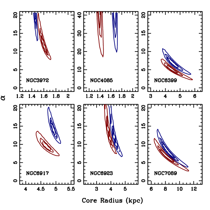
Figure 1: Likelihood maps of the best fit for the rotation curves of disk galaxies, treating the core radius (horizontal axis) and the TeVeS $\alpha$ parameter (vertical axis) as free parameters. The red (blue) contours correspond to the 75%, 90% and 95% confidence levels of the Chabrier (Salpeter) Initial Mass Function, respectively.

To calculate a possible dark matter component, a sample of double lensing systems from the CASTLES database  is analysed and the mass of the lensing galaxy in GR and TeVeS is calculated, using the same fully relativistic method outlined in Ref. msy . By comparing the mass from lensing to the stellar mass content calculated from a comparison of photometry and stellar population synthesis using a Chabrier Initial Mass Function (IMF), as in Ref. fsw05 , the mass deficit which belonged to the “dark” sector is found.

From the rotation curve analysis, the favoured values of $\alpha$ are $11.56$ and $8.54$ for Salpeter and Chabrier IMFs, respectively, and these values are examined in the context of lensing. The results from the lensing analysis are given in Table III.

				$Chab$	$Sal$	$\alpha=11.56_{-4.80}^{+12.77}~{}Sal$		$\alpha=8.54_{-6.1}^{+3.32}~{}Chab$		$\alpha=0$	$Chab$	$Sal$
Lens	$M_{*}^{Chab}$	$M_{*}^{Sal}$	$M_{GR}$	$\%DM$	$\%DM$	$M_{TeV}$	$\%DM$	$M_{TeV}$	$\%DM$	$M_{TeV}$	$\%DM$	$\%DM$
HS0818+1227	$16.2^{21.2}_{13.0}$	$20.8^{28.1}_{13.4}$	$32.71$	$50.5$	$36.4$	$30.59_{-0.92}^{+0.81}$	$30.0_{-2.1}^{+1.8}$	$30.11_{-1.00}^{+0.79}$	$46.2_{-1.9}^{+1.4}$	$19.1$	$15.2$	$-8.9$
FBQ0951+2635	$1.1^{2.1}_{0.5}$	$1.5^{3.0}_{0.8}$	$2.98$	$63.1$	$49.7$	$2.84_{-0.06}^{+0.05}$	$47.2_{-1.2}^{+0.9}$	$2.81_{-0.07}^{+0.05}$	$60.9_{-1.0}^{+0.6}$	$1.9$	$42.1$	$21.0$
HE1104-1805	$22.8^{51.2}_{12.7}$	$36.6^{63.7}_{23.1}$	$83.61$	$72.7$	$56.2$	$78.18_{-2.36}^{+2.10}$	$53.2_{-1.5}^{+1.2}$	$76.96_{-2.60}^{+2.02}$	$70.4_{-1.1}^{+0.7}$	$47.1$	$51.6$	$22.3$
LBQS1009-0252	$5.5^{7.9}_{4.2}$	$7.4^{9.8}_{5.0}$	$15.60$	$64.7$	$52.6$	$14.62_{-0.41}^{+0.98}$	$49.4_{-1.5}^{+3.2}$	$14.40_{-0.45}^{+0.36}$	$61.8_{-1.2}^{+0.9}$	$8.7$	$36.8$	$14.9$
HE2149-2745	$4.6^{6.7}_{3.6}$	$6.9^{8.9}_{5.0}$	$12.03$	$61.8$	$42.6$	$11.27_{-0.35}^{+0.29}$	$38.8_{-2.0}^{+1.1}$	$11.10_{-0.35}^{+0.28}$	$58.6_{-1.4}^{+1.0}$	$6.3$	$27.0$	$-9.5$

Table 3: $M_{*}$ is the stellar content of the lenses taken from FSans . The other columns show the masses of the lensing galaxies for GR and TeVeS when $\alpha=11.56$, $\alpha=8.54$ and $\alpha=0$. It is also given is the percentage of dark matter needed to account for the lensing observed given the luminous content of the galaxies. All masses are given in units of $10^{10}M_{\odot}$. The errors for the $\alpha=11.56$ and $\alpha=8.54$ are derived from the errors on the value of $\alpha$ and are given at the 95% confidence level.

Figure 2: Marginalised likelihood distributions with respect to the TeVeS $\alpha$ parameter for all six disk galaxies. The solid (dashed) lines correspond to the Chabrier (Salpeter) Initial Mass Function, respectively.

Figure 3: Total marginalised likelihood distributions with respect to the TeVeS $\alpha$ parameter combining the data for all six disk galaxies. The result for the Chabrier (Salpeter) IMF is shown as a solid (dashed) line.

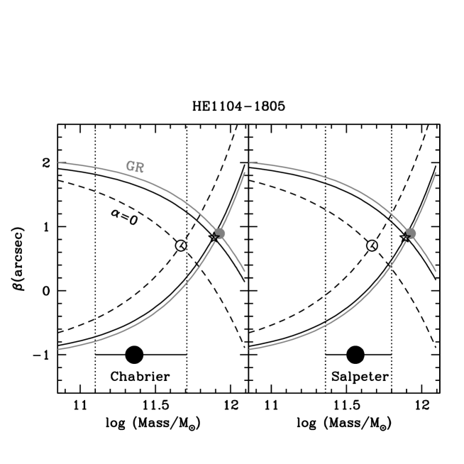
Figure 4: Constraining the lensing mass of galaxy HE1104-1805 (z$=0.73$). The lines come in pairs, and represent the constraint on true source position ($\beta$, vertical axis) and lensing mass (horizontal axis) from each of the two observed positions of the images of the background source. The intersection of each pair of lines give the lensing mass. The standard GR solution is shown as a grey solid line, the best fit is shown as a black solid line and the $\alpha=0$ case discussed in the text is given as a dashed black line. Each panel corresponds to a different choice of Initial Mass Function, as labelled. The stellar mass is given as a large black dot along with error bars, from Ref. fsw05 .

From Table III one can clearly conclude that when $\alpha=11.56$ and $\alpha=8.54$, there is a considerable need for dark matter, comparable to that required in the pure general relativistic case. We find that on average over the six galaxies, in the Salpeter case, TeVeS only predicts $3.4\%$ less dark matter than the general relativistic case: GR requires $47.5\%$ dark matter as opposed to TeVeS which requires $44.1\%$. For the Chabrier case TeVeS gives on average $59.6\%$ dark matter as opposed to GR which gives $62.6\%$, a reduction of only $5.0\%$. Using the errors on the value of $\alpha$, the errors on the mass are calculated at the $95\%$ confidence level. The error bars are quite tight, only $3.3\%$ on average in the Salpeter case and $2.2\%$ for Chabrier, showing just how strongly the analysis rules out this class of $\mu(y)$ functions. This result is in agreement with the work detailed in ref. msy , where it was shown that even for a value of $\alpha$ as low as 0 there is a not-insignificant need for dark matter. However the analysis presented in Ref. msy shows that only values of $\alpha$ greater than or equal to 1 can be definitively ruled out by the lensing data due to the error bars on the stellar masses. The $\alpha=0$ case is not ruled out as the lensing masses are within the error bars of the stellar masses, although they are consistently just within the upper error bar which suggests that with higher accuracy stellar mass estimates, even this case could be ruled out using just a lensing analysis. In the absence of more accurate estimates, we can test the $\alpha=0$ with rotation curves. Table II comparison of the $\chi^{2}$ for rotation curves for different values of $\alpha$. As it can be clearly seen, for three of our sample of six galaxies (N3972, N4085 and U6917), the $\alpha=0$ gives a value of $\chi^{2}$ which is nearly an order of magnitude larger than the best fit $\alpha$ case for both Salpeter and Chabrier IMFs, and is sufficiently high so as to be considered a poor fit. This implies that the $\alpha=0$ case is incompatible with rotation curves. This result was also suggested in Refs. mu1 ; mu2 where the authors showed, using a non-relativistic photometric fitting approach to rotation curves as opposed to the relativistic parametric fitting used here, that galaxy NGC3198 could not fit the data when $\alpha=0$ but only when $\alpha=1$, a case already ruled out by the lensing analysis of Ref. msy .

From this we can infer that there is no value of $\alpha$ which can satisfactorily fit both rotation curves and gravitational lensing. In conclusion, at the very least an entirely different form of the $\mu(y)$ function, and its related MONDian equivalent $f(x)$, needs to be found if the modifications to gravity are to remain universal in applicability with only the acceleration scale being free to be fitted.

V Conclusions and Outlook

In this paper we have made an attempt to constrain TeVeS models by using both gravitational lensing and rotation curve data. In particular, we have analysed the one-parameter models that have been fitted against the rotation curves, and we have found that there is no value of the parameter $\alpha$ that fits both the rotation curves and the gravitational lensing data of galaxies. The baryonic mass of the galaxies is calculated using photometric data and is assumed to account for the total mass budget of the system within the TeVeS paradigm. A standard likelihood method gives $\alpha=11.56_{-4.80}^{+12.77}$ for the Salpeter IMF, and $\alpha=8.54_{-6.1}^{+3.32}$ for the Chabrier IMF, at a 95% confidence level. Consequently, we estimate the mass content of five strong gravitational lenses from the CASTLES survey and compare their lensing masses to the corresponding stellar content, calculated from photometry. On taking into account the constraint from rotation curves, we find that the lensing mass within the TeVeS formalism still shows an excess around 50$\%$ over the baryonic content. The only successful parameter value from lensing ($\alpha=0$) is shown to be incompatible with rotation curves.

For the fits we used a particular set of galaxies, for which information for the inner part of the velocity distribution is available. The upshot of our analysis is that, at least in its simplest original form, which by the way is the only one studied in the literature so far, TeVeS is ruled out. One may think that multi-parametric extensions of TeVeS models may be successful. However, such models have not been proposed so far. Lacking a fundamental microscopic derivation of the $\mu$-functions, the use of such complicated models becomes unnatural and probably of no physical relevance.

Several features of the TeVeS model cannot be excluded at present, and in fact such features may be desirable and essential for fitting extended versions of TeVeS which include dark matter components. In particular, the bi-metric nature of TeVeS is an important ingredient which may indeed characterise more fundamental models, such as string-inspired foam ones nickmairi . Moreover, the vector-like cosmological instabilities implied by the vector time-like field $U^{\mu}$ may play an important rôle in structure formation, as emphasised in Ref. liguori , reconciling the observed baryonic spectrum with theoretical predictions. It is worthy of mentioning at this stage that in the context of the string models of Ref. nickmairi , the bi-metric feature of TeVeS is realised because of the presence of non-trivial dilaton fields, while the vector instabilities arise because of physical interactions of open string matter with space-time defects that such models include, as a result of the recoil of the latter. The models have a non-trivial dark energy component built in, as a result of the Born-Infeld-type dynamics of the vector field, that is characteristic in open string theories on brane worlds considered in that work. In addition, the string spectrum contains dark matter particles, in particular supersymmetric ones, and in this sense the TeVeS-like features co-exist with extra components of dark matter and dark energy in the model, fitting perfectly all currently available data, including cosmological ones. We should stress, however, that in such string models, the fundamental physics is entirely different, and even if one has TeVeS-like features, such as bi-metric models and vector-like instabilities, these are features that pre-existed the specific TeVeS models of Ref. bek and their origin is traced back to fundamental structures in string/brane framework.

Also, for reasons explained in Ref. nickmairi , an important rôle is played by neutrino matter in such models, which provide a significant component of dark matter, in addition to that offered by the supersymmetric matter. In this latter respect, we also mention other phenomenological works within the context of the TeVeS model or extensions thereof sko06 ; neutrinos , in a conventional field theoretic framework, claiming a prominent rôle of neutrinos as dark matter components in TeVeS-like models, fitting cosmological data. These are interesting avenues for research, which we intend and hope to be able to pursue in the near future.

References

- (1) See, e.g.: M. Tegmark et al. [SDSS Collaboration], Phys. Rev. D 74, 123507 (2006) [arXiv:astro-ph/0608632].
- (2) M. Milgrom, Astrophys. J. 270, 365 (1983).
- (3) J. D. Bekenstein, Phys. Rev. D 70, 083509 (2004) [Erratum-ibid. D 71, 069901 (2005)] [arXiv:astro-ph/0403694].
- (4) R.H. Sanders, Astrophys. J. 473, 117 (1996).
- (5) C. Skordis, D. F. Mota, P. G. Ferreira and C. Boehm, Phys. Rev. Lett. 96, 011301 (2006) [arXiv:astro-ph/0505519].
- (6) H. S. Zhao, D. J. Bacon, A. N. Taylor and K. Horne, Mon. Not. Roy. Astron. Soc. 368, 171 (2006) [arXiv:astro-ph/0509590].
- (7) M. Feix, C. Fedeli and M. Bartelmann, Astron. & Astrophysics 480, 313 (2008).
- (8) H. Shan, M. Feix, B. Famaey and H. Zhao, Mon. Not. Roy. Astron. Soc. 387, 1303 (2008) [arXiv:0804.2668 [astro-ph]].
- (9) N.E. Mavromatos, M. Sakellariadou and M. F. Yusaf, Phys. Rev. D 79, 081301(R) (2009) [arXiv:0901.3932 [astro-ph.GA]].
- (10) D. Giannios, Phys. Rev. D 71, 103511 (2005) [arXiv:gr-qc/0502122].
- (11) C. Skordis, arXiv:0903.3602 [astro-ph.CO].
- (12) L. Hernquist, Astrophys. J. 356, 359 (1990).
- (13) I. Ferreras, P. Saha and L. L. R. Williams, Astrophys. J. 623, L5 (2005) [arXiv:astro-ph/0503168].
- (14) J. R. Brownstein and J. W. Moffat, Astrophys. J. 636, 721 (2006) [arXiv:astro-ph/0506370].
- (15) H. Zhao, B. Famaey, Astrophys. J. 638, L9 (2006).
- (16) B. Famaey and J. Binney, Mon. Not. Roy. Astron. Soc. 363, 603 (2005) [arXiv:astro-ph/0506723].
- (17) G. W. Angus, B. Famaey and H. Zhao, Mon. Not. Roy. Astron. Soc. 371, 138 (2006) [arXiv:astro-ph/0606216].
- (18) M. A. W Verheijen, Astrophys. J. 563, 694-715 (2001)
- (19) M. A. W. Verheijen and R. Sancisi 2001, Astron. & Astrophys. 370, 765-867 (2001)
- (20) G. Bruzual and S. Charlot, Mon. Not. Roy. Astron. Soc. 344, 1000 (2003) [arXiv:astro-ph/0309134].
- (21) G. Bruzual, IAU No. 241 Symp. [arXiv:astro-ph/0703052] (2007)
- (22) G. Chabrier, Publ. Astron. Soc. Pac. 115, 763 (2003) [arXiv:astro-ph/0304382].
- (23) E. E. Salpeter, Astrophys. J. 121, 161 (1955)
- (24) I. Ferreras, M. Sakellariadou and M. F. Yusaf, Phys. Rev. Lett., 100, 031302 (2008).
- (25) I. Ferreras, P. Saha and S. Burles, Mon. Not. Roy. Astron. Soc. 383, 857 (2008).
- (26) M. Cappellari, et al., Mon. Not. Roy. Astron. Soc. 366, 1126 (2006).
- (27) R. H. Sanders and D. D. Land, arXiv:0803.0468 [astro-ph].
- (28) R. Narayan and M. Bartelmann, Lectures on Gravitational Lensing (1996), arXiv:astro-ph/9606001.
- (29) N. E. Mavromatos and M. Sakellariadou, Phys. Lett. B 652, 97 (2007) [arXiv:hep-th/0703156].
- (30) S. Dodelson and M. Liguori, Phys. Rev. Lett. 97, 231301 (2006) [arXiv:astro-ph/0608602].
- (31) see e.g.: G. Gentile, H. S. Zhao and B. Famaey, arXiv:0712.1816 [astro-ph]; G. W. Angus, H. Shan, H. Zhao and B. Famaey, Astrophys. J. 654, L13 (2007) [arXiv:astro-ph/0609125].