Detecting Relic Gravitational Waves in the CMB: Comparison of Planck and Ground-based Experiments

Abstract

We compare the detection abilities for the relic gravitational waves by two kinds of forthcoming cosmic microwave background radiation (CMB) experiments, space-based Planck satellite and the various ground-based experiments. Comparing with the ground-based experiments, Planck satellite can observe all the CMB power spectra in all the multipole range, but having much larger instrumental noises. We find that, for the uncertainty of the tensor-to-scalar ratio $\Delta r$, PolarBear (II) as a typical ground-based experiment can give much smaller value than Planck satellite. However, for the uncertainty of the spectral index $\Delta n_{t}$, Planck can give the similar result with PolarBear (II). If combining these two experiments, the value of $\Delta n_{t}$ can be reduced by a factor $2$. For the model with $r=0.1$, the constraint $\Delta n_{t}=0.10$ is expected to be achieved, which provides an excellent opportunity to study the physics in the very early universe. We also find the observation in the largest scale ($\ell<20$) is very important for constraining the spectral index $n_{t}$. So it is necessary to combine the observations of the future space-based and ground-based CMB experiments to determine the relic gravitational waves.

I Introduction

Relic gravitational waves (RGWs) are generated in the very early Universe due to the superadiabatic amplification of zero point quantum fluctuations of the gravitational field a1 ; s2 , and freely evolve in the whole stage of the Universe zhao ; others . So RGWs carry invaluable information about early history of our Universe inaccessible to any other medium.

Detection of RGWs is rightly considered a highest priority for the upcoming cosmic microwave background radiation (CMB) experiments. The current CMB experiments are yet to detect a definite signature of RGWs experiment1 . In the near future, the successive generation of the experiments, including the space-based Planck satellite Planck and the various ground-based experiments bicep ; polarbear ; quiet ; experiment2 together with a host of balloon-borne experiments balloon will provide an increasing sensitive measurement of RGWs.

The space-based experiments, as COBE, WMAP and Planck satellites, can remove atmospheric noises and observe the fairly cleaned CMB temperature and polarization anisotropy fields. In addition, the space-based experiments provide the unique opportunity to detect the CMB power spectra in the largest scale ($\ell<20$) by surveying the full sky.

At the same time, the CMB polarization field can also be observed by the ground-based experiments. Since the atmospheric emission is not expected to be linearly polarized keating1998 , by integrating deeply on the relatively small patches of sky, it is possible to make a measurement of the polarization anisotropies with a comparable signal-to-noise ratio to a satellite experiment on all but the largest angular scales.

In this letter, we shall investigate the detection abilities for the RGWs, by the observations of the forthcoming generation of the ground-based and space-based experiments. By calculating the constraints on the tensor-to-scalar ratio $r$ and the tensor spectral index $n_{t}$, we shall compare the detection abilities of these two types of experiments. We also investigate the potential improvement of the detection ability by combining the observations of them.

II Review of primordial perturbations, CMB and noises

II.1 Primordial perturbation power spectra

The main contribution to the temperature and polarization anisotropies of the CMB comes from two types of cosmological perturbations, density perturbations (also known as the scalar perturbations) and RGWs (also known as the tensor perturbations). The primordial power spectra of these perturbations are usually assumed to be power laws, which is a generic prediction of a wide range of scenarios of the early Universe lyth . If we ignore the running of the spectral indices, the primordial spectra can be written as the following simple forms

$$P_{{s}}(k)=A_{s}(k_{0})\left({k}/{k_{0}}\right)^{n_{s}-1},$$ (1)

$$P_{t}(k)=A_{t}(k_{0})\left({k}/{k_{0}}\right)^{n_{t}},$$ (2)

where $k_{0}$ is the pivot wavenumber, which can be arbitrarily chosen. $n_{s}$ and $n_{t}$ are the scalar and tensor spectral indices. The tensor-to-scalar ratio is defined by

$$r(k_{0})\equiv\frac{A_{t}(k_{0})}{A_{s}(k_{0})}.$$ (3)

For a fixed $A_{s}$, the primordial power spectra of RGWs are completely determined by two parameters $r$ and $n_{t}$, if a power-law form in (2) is assumed. The simplest single-field slow-roll inflationary models predict a consistency relation between $r$ and $n_{t}$ lyth : $n_{t}=-r/8$. However, this consistency relation is incorrect for other inflationary models othermodels . So the determination the parameters $r$ and $n_{t}$ by the observations, provides an excellent opportunity to distinguish various inflationary-type models.

Since in this letter, we are primarily interested in the parameters of the RGW field, in the analysis below we shall work with a fixed cosmological background model. More specifically, we shall work in the framework of $\Lambda$CDM model, and keep the background cosmological parameters fixed at the values determined by a typical model typical

$$\begin{array}[]{c}h=0.732,~{}\Omega_{b}h^{2}=0.02229,\\ \Omega_{m}h^{2}=0.1277,~{}\Omega_{k}=0,~{}\tau_{reion}=0.089.\end{array}$$ (6)

Furthermore, in order to show the results in the figures, we adopt the following parameters of the density perturbations and tensor spectral index,

$$A_{s}=2.3\times 10^{-9},~{}n_{s}=1,~{}n_{t}=0.$$ (7)

II.2 CMB power spectra and their estimators

Let us turn our attention to the CMB field. Density perturbations and gravitational waves produce temperature and polarization anisotropies in the CMB characterized by four angular power spectra $C_{\ell}^{T}$, $C_{\ell}^{E}$, $C_{\ell}^{B}$ and $C_{\ell}^{C}$ as functions of the multipole number $\ell$ a8 ; grishchuk-cmb ; a10 ; a11 . Here $C_{\ell}^{T}$ is the power spectrum of the temperature anisotropies, $C_{\ell}^{E}$ and $C_{\ell}^{B}$ are the power spectra of the so-called $E$-mode and $B$-mode polarizations and $C_{\ell}^{C}$ is the power spectrum of the temperature-polarization cross correlation.

In the linear theory, the various power spectra $C_{\ell}^{Y}$ (where $Y=T,E,B$ or $C$) can be presented in the following form

$$C_{\ell}^{Y}=C_{\ell,s}^{Y}+C_{\ell,t}^{Y},$$ (8)

where $C_{\ell,s}^{Y}$ are the power spectra due to the density perturbations, and $C_{\ell,t}^{Y}$ are the power spectra due to RGWs.

The CMB power spectra $C_{\ell}^{Y}$ are theoretical constructions determined by ensemble averages over all possible realizations of the underlying random process. However, in real CMB observations, we only have access to a single sky, and hence to a single realization. In order to obtain information on the power spectra from a single realization, it is required to construct estimators of power spectra $D_{\ell}^{Y}$ ours1 . The probability distribution functions for the estimators are detailed described in ours1 , which predicts the expectation values of the estimators

$$\langle D_{\ell}^{Y}\rangle=C_{\ell}^{Y},$$ (9)

and the standard deviations ours1

$$\begin{array}[]{c}(\sigma_{D_{\ell}^{X}})^{2}=\frac{2(C_{\ell}^{X}+N_{\ell}^{X})^{2}}{(2\ell+1)f_{\rm sky}},~{}~{}(X=T,E,B)\\ (\sigma_{D_{\ell}^{C}})^{2}=\frac{(C_{\ell}^{T}+N_{\ell}^{T})(C_{\ell}^{E}+N_{\ell}^{E})+(C_{\ell}^{C})^{2}}{(2\ell+1)f_{\rm sky}},\end{array}$$ (12)

where $f_{\rm sky}$ is the cut-sky factor, and $N_{\ell}^{X}$ are the noise power spectra, determined by the specific experiments .

II.3 Noise power spectra

Considering an experiment with multiple frequency channels, the total instrumental noise power spectra can be approximately presented as (see for instance ground ),

$$N_{\ell}^{X}=\left(\sum_{c}\frac{1}{N_{\ell,c}^{X}}\right)^{-1}.$$ (13)

Here $N_{\ell,c}^{X}$ is the noise power spectrum for the individual frequency channel, which is given by

$$N_{\ell,c}^{X}=(\sigma_{pix}^{X}\cdot\theta_{\rm F})^{2}\cdot\exp\left[\ell(\ell+1)\frac{\theta_{\rm F}^{~{}2}}{8\ln 2}\right].$$ (14)

In this formula, $\theta_{\rm F}$ is the full width half maximum (FWHM) beam size. The pixel noises $\sigma_{pix}^{X}$ depend on the survey design and the instrumental parameters.

First, let us focus on the space-based Planck satellite. In this paper, we consider four frequency channels for the Planck satellite, which are listed in Table 1. After two full sky survey (14 months), the pix noises $\sigma_{pix}^{X}$ are expected to be the values listed in Table 1 for different channels. In FIG.1, we plot the instrumental noise power spectrum $N_{\ell}^{B}$, as a comparison with the values of CMB power spectrum $C_{\ell}^{B}$ in the model with $r=0.1$ and $r=0.01$. We find, in the model of $r=0.1$, the value of $C_{\ell}^{B}$ is larger than that of $N_{\ell}^{B}$ only at the largest scale. So Planck satellite can detect RGWs mainly by the observation in this largest scale, which will be clearly shown in the following section.

For a ground-based experiment with $N_{d}$ detectors, a solid angle per pixel $\theta_{\rm F}^{~{}2}$ and a sensitivity NET, we assume it will survey an area $4\pi f_{\rm sky}$ in the integration time $t_{obs}$. The pixel polarization noises are

$$(\sigma_{pix}^{E})^{2}=(\sigma_{pix}^{B})^{2}=\frac{(\sqrt{2}{\rm NET})^{2}\cdot 4\pi f_{\rm sky}}{t_{obs}N_{d}~{}\theta_{\rm F}^{~{}2}}.$$ (15)

In this paper, we shall discuss five kinds of ground-based experiments: BICEP, PolarBear (I) and (II), QUIET (I) and (II). The instrumental parameters for these experiments are given in the Appendix A. Notice that, the ground-based experiments are only sensitive to the polarizations. Since the ground-based experiments can only survey a small part of the full sky, it cannot encode the information of CMB field in the very large scale. From FIG.1, we find that ground-based experiments have much smaller noise power spectra than Planck satellite.

We should notice that, cosmic lensing can convert the $E$-mode polarization into $B$-mode (see lens for a review). So the $B$-mode spectrum due to RGWs will be contaminated by a cosmic lensing contribution. The lensed $C_{\ell}^{B}$ is also shown in FIG.1, which can be treated as a part of the total noise power spectrum $N_{\ell}^{B}$ as well as instrumental noise power spectra in (13).

In addition to the instrumental noises and lensing noise, various foregrounds, such as the synchrotron and dust, are also the important contaminations in the CMB observation. It is hoped that the multifrequency observations and the hard work by astronomical community might allow future experiments can reduce the foreground noises in a very accurate level (see for instance foreground ). So in the following discussion, we shall not consider this kind of contamination.

Table 1: Instrumental parameters for Planck satellite Planck .

Band center [GHz]	100	143	217
$\sigma_{pix}^{T}$ [$\mu$K]	6.8	6.0	13.1
$\sigma_{pix}^{E}$ and $\sigma_{pix}^{B}$ [$\mu$K]	10.9	11.5	26.8
FWHM [arcmin]	$9.5$	$7.1$	$5.0$
$f_{\rm sky}$	$0.65$
$\ell$ range	$2\sim 1000$
Integration time	$14$ Months

Figure 1: This figure shows the instrumental noise power spectrum $N_{\ell}^{B}$ for Planck satellite and various ground-based experiments (solid lines). For the comparison, we also plot the power spectra $C_{\ell}^{B}$ in the models with $r=0.1$ and $r=0.01$ (magenta dashed lines). The blue dotted line denotes the power spectra $C_{\ell}^{B}$ generated by cosmic lensing.

III Determination of RGWs by CMB observations

In the previous works ours1 ; ours2 ; ours3 , we have discussed how to best constrain the parameters of the RGWs, i.e. $r$ and $n_{t}$, by the CMB observation. In the paper ours3 , we found that, in general the constraints on $r$ and $n_{t}$ correlate with each other. However, if we consider the tensor-to-scalar ratio at the best-pivot wavenumber $k_{t}^{*}$, i.e. $r\equiv r(k_{t}^{*})$, the constraints on $r$ and $n_{t}$ becomes independent of each other, and the uncertainties $\Delta{r}$ and $\Delta{n_{t}}$ have the minimum values. In the work ours3 , we have derived the formulas to calculate the quantities: the best-pivot wavenumber $k_{t}^{*}$, and the uncertainties of the parameters $\Delta r$ and $\Delta{n_{t}}$. This provides a simple and quick method to investigate the ability of the CMB observations for the detect of RGWs. In this section, we shall briefly introduce these results.

It is convenient to define two quantities as below,

$$a_{\ell}^{Y}\equiv\frac{C_{\ell,t}^{Y}}{\sigma_{D_{\ell}^{Y}}},~{}~{}b^{*}_{\ell}\equiv\ln\left(\frac{\ell}{\ell_{t}^{*}}\right).$$ (16)

Here $C_{\ell,t}^{Y}$ are the CMB power spectra generated by RGWs, and $\sigma_{D_{\ell}^{Y}}$ are the standard deviations of the estimators $D_{\ell}^{Y}$, which can be calculated by Eq.(12). $\ell_{t}^{*}$ is the best-pivot multipole, which is determined by solving the following equation ours3 :

$$\sum_{\ell}\sum_{Y}a_{\ell}^{Y2}b_{\ell}^{*}=0.$$ (17)

So the value of $\ell_{t}^{*}$ depends on the cosmological model, the amplitude of RGWs, and the noise power spectra. The best-pivot wavenumber $k_{t}^{*}$ relates to $\ell_{t}^{*}$ by the approximation ours3 ,

$$k_{t}^{*}\simeq\ell_{t}^{*}\times 10^{-4}{\rm Mpc}^{-1}.$$ (18)

In order to determine the constraints on the RGWs from the CMB observation, we can consider two quantities, the signal-to-noise ratio $S/N$ (which directly relate to $\Delta r$) and uncertainty $\Delta n_{t}$. For a specific cosmological model and the noises, these quantities can be calculated by the following formulas ours1 ; ours2 ; ours3

$$\begin{array}[]{c}S/N\equiv{r}/{\Delta r}=\sqrt{\sum_{\ell}\sum_{Y}a_{\ell}^{Y2}},\\ \Delta n_{t}=1/\sqrt{\sum_{\ell}\sum_{Y}(a_{\ell}^{Y}b_{\ell}^{*})^{2}}.\end{array}$$ (21)

In this letter, in order to compare the detection abilities for RGWs of Planck and the ground-based experiments, we shall consider the following four cases:

Case A: We only consider the observation of the $B$-polarization by Planck satellite. So, in Eqs. (17) and (21), $Y=B$ and $\ell=2\sim 1000$. The noise power spectrum $N_{\ell}^{B}$ and cut sky factor $f_{\rm sky}$ are the corresponding quantities for Planck satellite.

Case B: We only consider the observation of the $B$-polarization by the ground-based experiments.

Case C: We consider the determination on the RGWs by combining the $B$-polarization observations of Planck and the various ground-based experiments. Since the power spectra in the scale $\ell<20$ ($\ell<30$ for PolarBear (I)) can only be observed by Planck satellite, we adopt the $N_{\ell}^{B}$ and $f_{\rm sky}$ as the the corresponding quantities for Planck satellite. In the scale $\ell=20\sim 1000$ ($\ell=30\sim 1000$ for PolarBear (I)), we only adopt the $N_{\ell}^{B}$ and $f_{\rm sky}$ as the corresponding quantities for ground-based experiments.

Case D: In addition to the $B$-polarization discussed in Case C, we also take into account the observations of the other three power spectra, i.e. $Y=T,C,E$. For $Y=T$ and $C$, only observed by Planck satellite, we consider the Planck noises and cut sky factor. For $Y=E$, similar with $Y=B$, Planck noise and cut sky factor are considered for $\ell<20$ ($\ell<30$ for PolarBear (I)), and the noises and cut sky factors of ground-based experiments are considered for the other multipole scales.

III.1 Best-pivot multipole $\ell_{t}^{*}$

Figure 2: This figure shows the best-pivot multipole $\ell_{t}^{*}$ for Planck and PolarBear (II) experiments in Case A (red line), Case B (black line), Case C (blue line) and Case D (green line).

Figure 3: This figure shows the best-pivot multipole $\ell_{t}^{*}$ in Case D for the various ground-based experiments.

First, let us discuss PolarBear (II) as a typical ground-based experiment. By solving Eq.(17), in FIG.2 we plot the best-pivot multipole $\ell_{t}^{*}$ as a function of tensor-to-scalar ratio $r$ in the four cases. In Case A, the value of $\ell_{t}^{*}$ is always smaller than $40$, which is because that, in Case A the main contribution on the constraint of RGWs only comes from the observation in the very large scale, i.e. the reioniation peak of $B$-polarization power spectrum ours1 ; ours2 . In Case B, $50<\ell_{t}^{*}<130$, the best-pivot multipole is in the intermedial scale, which reflects that PolarBear (II) constrains the RGWs mainly by the observation in the intermedial scale. As a combination of Case A and B, in Case C the value of $\ell_{t}^{*}$ is focused on the range $40<\ell_{t}^{*}<90$. If we also consider the other three power spectra, $T,E,C$ in Case D, the value of $\ell_{t}^{*}$ decreases a little when $r>0.1$, due to the contribution of $T,E,C$ power spectra ours2 .

In FIG. 3, we also plot the best-pivot multipole $\ell_{t}^{*}$ as a function of $r$ in Case D, where the various ground-based experiments are considered. In all these cases, we find that the value of $\ell_{t}^{*}$ increases with the increasing of $r$. In general, the smaller instrumental noises follow the larger $\ell_{t}^{*}$.

III.2 Signal-to-noise ratio $S/N$

Figure 4: This figure shows the signal-to-noise ratio $S/N$ for Planck and PolarBear (II) experiments in Case A (red line), Case B (black line), Case C (blue line) and Case D (green line).

Figure 5: The figure shows the signal-to-noise ratio $S/N$ in Case D for the various ground-based experiments.

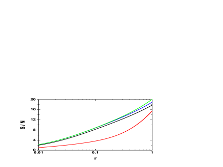
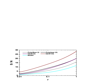
FIG.4 presents the signal-to-noise ratio $S/N$ as a function of $r$ for Planck and PolaeBear (II) experiments, which are obtained by using the first formula in Eq.(21). As expected, in all these four cases, a larger $r$ predicts a larger $S/N$. When $r=0.1$, $S/N=3.6$ for Planck satellite, and $S/N=8.4$ for PolarBear (II) experiment. If we require that $S/N>3$, $r>0.07$ must be satisfied for Planck satellite, and $r>0.02$ for PolarBear (II) experiment. This figure shows that, PolarBear (II) can give a much tighter constraint of $r$ than Planck satellite, due to the much smaller noise level of the PolarBear (II) experiment. Even if we combine Planck and PolarBear (II) experiments, the constraint on $r$ cannot make obvious improvement.

In FIG. 5, we also plot the $S/N$ as a function of $r$ in Case D, where the various ground-based experiments are considered. As expected, the values $S/N$ strongly depend on the instrumental noises and the sky survey factor $f_{\rm sky}$ of the ground-based experiments. The QUIET (II) can very well detect the signal of RGWs ($4$-$\sigma$ level), even for the model with $r=0.01$,

Figure 6: In the model of $r=0.1$ for Planck and PolarBear (II) experiment, we plot the individual signal-to-noise ratio $(S/N)^{2}_{\ell}$ as a function of multipole $\ell$ in Case A (red line), Case B (black line), Case C (blue line) and Case D (green line).

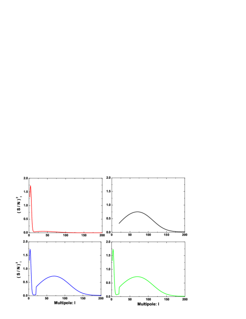
From the first formula in (21), we find the total signal-to-noise ratio can be written as $(S/N)^{2}=\sum_{\ell}(S/N)_{\ell}^{2}$, where the individual signal-to-noise ratio for the multipole $\ell$ is $(S/N)_{\ell}^{2}=\sum_{Y}a_{\ell}^{Y2}$. FIG.6 presents the quantity $(S/N)_{\ell}^{2}$ as a function of multipole $\ell$ in the model with parameter $r=0.1$. This figure clearly shows that, for the Planck satellite the constraint on $r$ mainly comes from the observation in the reionization peak at $\ell<10$, and for PolarBear (II) experiment, the constraint mainly comes from the observation in the intermedial scale $20<\ell<150$. In Case C and D, the function $(S/N)_{\ell}^{2}$ has two peaks, one is at $\ell<10$, and the other is at $\ell\sim 80$. Comparing with the second peak, the first peak, due to the observation of Planck satellite, is very narrow, and only contribute a fairly smalle portion for the total $S/N$. From FIG.6, we also find the difference between Case C and D is only at the range $10<\ell<20$, due to the observation of the $Y=T,E$ and $C$ power spectra.

III.3 Uncertainty of spectral index $\Delta n_{t}$

Now, let us turn our attention to the constraint of the tensor spectral index $n_{t}$. Inserting the best-pivot multipole $\ell_{t}^{*}$ into the second formula in Eq.(15) and taking into account the corresponding noise power spectra, we obtain the $\Delta n_{t}$ as a function of $r$, which are presented in FIG.7. In this figure, we have considered the Planck and PolarBear (II) experiments. We find that, the value of $\Delta n_{t}$ in Case A is similar with that in Case B, although the Planck noise $N_{\ell}^{B}$ is nearly 300 times larger than that of PolarBear (II). When $r>0.08$, Planck can give a tighter constraint, and when $r<0.08$, PolarBear (II) can give a tighter constraint. When $r=0.1$, we find $\Delta n_{t}=0.23$ for Case A, and $\Delta n_{t}=0.24$ for Case B. Both of them are fairly large for the constraint of the inflationary models. The single-field slow-roll inflationary models predict the consistency relation $n_{t}=-r/8$ lyth , which provides the unique way to exactly test or rule out this kind of models. In order to answer: whether the observations provide the probability to check the consistency relation, we can compare the values of $\Delta n_{t}$ with $r/8$. If $\Delta n_{t}<r/8$, we can say the constraint on $n_{t}$ is tight enough to check the consistency relation. From FIG.7, we find that $\Delta n_{t}<r/8$ is satisfied only if $r>0.9$ for Case A, and $r>0.8$ for Case B. Unfortunately, these models have been safely excluded by the current observations currentconstraint . So we conclude that, by either of the single experiment, Planck or PolarBear (II), we cannot constrain $n_{t}$ tight enough to check the consistency relation.

Figure 7: This figure shows the uncertainty $\Delta n_{t}$ for Planck and PolarBear (II) experiments in Case A (red line), Case B (black line), Case C (blue lines) and Case D (green lines). The dashed (magenta) line denote the line with $\Delta n_{t}=r/8$.

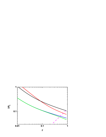
Now, let us consider Case C, which has combined the Planck and PolarBear (II) experiments. We find in this case, the constraint on $n_{t}$ becomes much tighter than that in Case A or B. Comparing with Case B, the value of $\Delta n_{t}$ is reduced by a factor $2$. When $r=0.1$, $\Delta n_{t}=0.10$, which is much smaller than that in Case A or B. From FIG.7, we also find that $\Delta n_{t}<r/8$ is satisfied only if $r>0.5$. If considering the contribution of $T,E,C$, i.e. Case D, the constraint on $n_{t}$ can be even reduced when $r>0.2$. So combining the Planck and PolarBear (II) experiments can effectively reduce the uncertainty of $n_{t}$, although the noise power spectra of Planck experiment is much larger than that in PolarBear (II).

Figure 8: The figure shows the uncertainty $\Delta n_{t}$ in Case D for the various ground-based experiments.

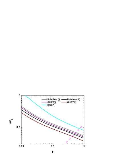
In FIG. 8, we also plot the $\Delta n_{t}$ as a function of $r$ in Case D, where the various ground-based experiments are considered. We find that, by combing QUIET (II) and Planck experiments, we can get a constraint $\Delta n_{t}=0.09$ for the model with $r=0.1$, and a constraint $\Delta n_{t}=0.06$ for the model with $r=0.3$.

Figure 9: In the model of $r=0.1$ for Planck and PolarBear (II) experiments, we plot the quantities of $\sum_{Y}(a_{\ell}^{Y}b_{\ell}^{*})^{2}$ as a function of multipole $\ell$ in Case A (red line), Case B (black line), Case C (blue line) and Case D (green line).

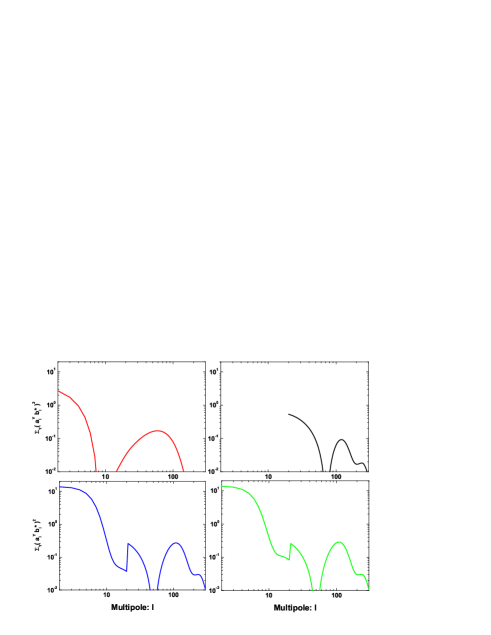
Let us investigate the contribution of the observation in the individual multipole $\ell$. From Eq.(15), we find the quantity $(1/\Delta n_{t})^{2}$ is a sum of $\sum_{Y}(a_{\ell}^{Y}b_{\ell}^{*})^{2}$ for the multipole $\ell$. In FIG.9 we plot the quantity $\sum_{Y}(a_{\ell}^{Y}b_{\ell}^{*})^{2}$ as a function of $\ell$ for all the four cases, where we have considered the model with parameter $r=0.1$. In all cases, the contribution on the constraint of $\Delta n_{t}$ mainly comes from the observation in the rage $\ell<300$. From this figure, we also find that this quantity has the zero value when $\ell=\ell_{t}^{*}$, due to $b_{\ell}^{*}(\ell=\ell_{t}^{*})=0$. So the observation around the best-pivot multipole is not important for the constraint of $n_{t}$. In the range of $\ell<300$, when $\ell\ll\ell_{t}^{*}$ or $\ell\gg\ell_{t}^{*}$, the value of $b_{\ell}^{*}$ is large, as well as the quantity $\sum_{Y}(a_{\ell}^{Y}b_{\ell}^{*})^{2}$, which gives the important contribute for the constraint of $n_{t}$. Especially the observation in the largest scale. For instance, in Case C the best-pivot multipole $\ell_{t}^{*}=51$, so $(b_{\ell=2}^{*})^{2}=10.5$ and $(b_{\ell=200}^{*})^{2}=1.86$, the former one is 6 times larger than the latter one. So the observation at $\ell=2$ is much more important than that at $\ell=200$, for constraining the spectral index $n_{t}$. We conclude that, the Planck observation in the largest scale is extremely important for the constraint of $n_{t}$, although the noise power spectra of Planck satellite is much larger than that of the ground-based experiments.

IV Conclusion

Detecting the signal of RGWs is one of the most important tasks for the forthcoming CMB experiments, including the ground-based, space-based and balloon-borne experiments. In this letter, by calculating the uncertainty of the parameters $r$ and $n_{t}$, we compared the detection abilities of the upcoming space-based Planck mission and the various ground-based experiments. Comparing with Planck experiment, ground-based experiments have the much smaller instrumental noise power spectra, but can only observe the CMB field for a small portion of full sky.

We find that ground-based experiments predict a much larger $S/N$ for all the inflationary models, by observing the CMB power spectra in the intermedial multipole range. Even we combine it with Planck experiment, the value of $S/N$ cannot be obviously improved.

By calculating the value of $\Delta n_{t}$, we find ground-based experiments have the similar ability with Planck mission for the determination of $n_{t}$. If combining them, the value of $\Delta n_{t}$ can be much reduced, which provides an excellent opportunity to distinguish the various inflationary models. We also find that, the observation in the largest scale ($\ell<20$) is extremely important for determining the spectral index $n_{t}$.

Acknowledgement:

W.Zhao thanks NAOC and BNU for invitation and hospitality. This work is supported by Chinese NSF under grant Nos. 10703005 and 10775119. In this paper, we have used the CAMB code for the calculation of CMB power spectra camb .

Appendix A Instrumental parameters of the various ground-based experiments

In this appendix, we shall list the instrumental parameters for the various ground-based experiment, which including BICEP, PolarBear (I) and (II), QUIET (I) and (II). The parameters are detailed listed in Tables 2$-$6, separately.

Table 2: Instrumental parameters for BICEP experiment bicep .

Band center  [GHz]	97.7	151.8
$N_{d}$	50	48
NET [$\mu$K$\cdot$ sec${}^{\frac{1}{2}}$]	480	420
FWHM [arcmin]	$55$	$37$
$f_{\rm sky}$	$0.024$
$\ell$ range	$20\sim 1000$
Integration time	$380$ Days

Table 3: Instrumental parameters for PolarBear (I) experiment polarbear .

Band center  [GHz]	90	150	220
$N_{d}$	104	160	96
NET [$\mu$K$\cdot$ sec${}^{\frac{1}{2}}$]	220	244	453
FWHM [arcmin]	$6.7$	$4.0$	$2.7$
$f_{\rm sky}$	$0.012$
$\ell$ range	$30\sim 1000$
Integration time	$0.45$ Years

Table 4: Instrumental parameters for PolarBear (II) experiment polarbear .

Band center  [GHz]	90	150	220
$N_{d}$	400	600	200
NET [$\mu$K$\cdot$ sec${}^{\frac{1}{2}}$]	220	244	453
FWHM [arcmin]	$6.7$	$4.0$	$2.7$
$f_{\rm sky}$	$0.024$
$\ell$ range	$20\sim 1000$
Integration time	$0.45$ Years

Table 5: Instrumental parameters for QUIET (I) experiment quiet .

Band center  [GHz]	40	90
$N_{d}$	19	91
NET [$\mu$K$\cdot$ sec${}^{\frac{1}{2}}$]	160	250
FWHM [arcmin]	$23$	$10$
$f_{\rm sky}$	$0.04$
$\ell$ range	$20\sim 1000$
Integration time	$2$ Years

Table 6: Instrumental parameters for QUIET (II) experiment quiet .

Band center  [GHz]	40	90
$N_{d}$	1000	1000
NET [$\mu$K$\cdot$ sec${}^{\frac{1}{2}}$]	160	250
FWHM [arcmin]	$23$	$10$
$f_{\rm sky}$	$0.04$
$\ell$ range	$20\sim 1000$
Integration time	$3$ Years

References

- (1) L. P. Grishchuk, Zh. Eksp. Teor. Fiz. 67 (1974) 825 [Sov. Phys. JETP 40 (1975) 409]; Ann. NY Acad. Sci. 302 (1977) 439; Pis’ma Zh. Eksp.Teor. Fiz. 23 (1976) 326 [JETP Lett. 23 (1976) 293].
- (2) A. A. Starobinsky, JEPT Lett. 30 (1979) 682; V. A. Rubakov, M. V. Sazhin and A. V. Veryashin, Phys. Lett. B 115 (1982) 189; R. Fabbri and M. D. Pollock, Phys. Lett. B 125 (1983) 445; L. F. Abbott and M. B. Wise, Nucl. Phys. B 224 (1984) 541; L. F. Abbott and D. D. Harari, Nucl. Phys. B 264 (1986) 487.
- (3) L. P. Grishchuk, Lect. Notes Phys. 562 (2001) 167; Y. Zhang, Y. F. Yuan, W. Zhao and Y. T. Chen, Class. Quant. Grav. 22 (2005) 1383; W. Zhao and Y. Zhang, Phys. Rev. D 74 (2006) 043503; T. L. Smith, H. V. Peiris and A. Cooray, Phys. Rev. D 73 (2006) 123503.
- (4) N. Seto and J. Yokoyama, Journal of the Physical Society of Japan 72 (2003) 3082; Y. Watanabe and E. Komatsu, Phys. Rev. D 73 (2006) 123515; W.Zhao, Chinese Physics 16 (2007) 2894; K. Nakayama, S. Saito, Y. Suwa and J. Yokoyama, JCAP 0806 (2008) 020; L. A. Boyle and P. J. Steinhardt, Phys. Rev. D 77 (2008) 063504; K. Nakayama, S. Saito, Y. Suwa and J. Yokoyama, Phys. Rev. D 77 (2008) 124001; M. Giovannini, Phys. Lett. B 668 (2008), 44.
- (5) C. J. MacTavish et al., Astrophys. J. 647 (2006) 799; N. Rajguru et al., Mon. Not. R. Astron. Soc. 363 (2005) 1125; CAPMAP Collaboration, Astrophys. J. 684 (2008) 771; E. M. Leitch et al., Astrophys. J. 624 (2005) 10; QUaD Collaboration, Astrophys. J. 692 (2009) 1247; M. R. Nolta et al., Astrophys. J. Suppl. 180 (2009) 296.
- (6) Planck Collaboration, The Science Programme of Planck [arXiv:astro-ph/0604069].
- (7) K. W. Yoon et al., astro-ph/0606278.
- (8) http://bolo.berkeley.edu/polarbear/index.html.
- (9) http://quiet.uchicago.edu/index.php; D. Samtleben, arXiv:0802.2657.
- (10) http://groups.physics.umn.edu/cosmology/ebex/index.html; http://www.iac.es/project/cmb/quijote/.
- (11) A. Kogut et al., New Astron.Rev. 50 (2006) 1009; B. P. Crill et al., arXiv:0807.1548.
- (12) B. Keating, P. Timbie, A. Polnarev and J. Steinberger, Astrophys. J. 495 (1998) 580.
- (13) D. H. Lyth and A. Riotto, Phys. Rep. 314 (1999) 1.
- (14) D. Polarski and A. A. Starobinsky, Phys. Lett. B 356 (1995) 196; L. P. Grishchuk, Phys. Usp. 48 (2005) 1235 [Usp. Fiz. Nauk. 175 (2005) 1289]; R. H. Brandenberger, A. Nayeri, S. P. Patil and C. Vafa, Phys. Rev. Lett. 98 (2007) 231302; J. Grain and A. Barrau, Phys. Rev. Lett. 102 (2009) 081301.
- (15) D. N. Spergel et al., Astrophys. J. Suppl. 170 (2007) 377.
- (16) A. Polnarev, Sov. Astron. 29 (1985) 607; D. Harari and M. Zaldarriaga, Phys. Lett. B 310 (1993) 96; U. Seljak and M. Zaldarriaga, Phys. Rev. Lett. 78 (1997) 2054; M. Kamionkowski, A. Kosowsky and A. Stebbins, Phys. Rev. D 55 (1997) 7368.
- (17) L. P. Grishchuk, Phys. Rev. D 48 (1993) 5581; Phys. Rev. Lett. 70 (1993) 2371.
- (18) M. Zaldarriaga and U. Seljak, Phys. Rev. D 55 (1997) 1830.
- (19) J. R. Pritchard and M. Kamionkowski, Ann. Phys. (N.Y.) 318 (2005) 2; W. Zhao and Y. Zhang, Phys. Rev. D 74 (2006) 083006; D. Baskaran, L. P. Grishchuk and A. Polnarev, Phys. Rev. D 74 (2006) 083008; B. G. Keating, A. G. Polnarev, N. J. Miller and D. Baskaran, Int. J. Mod. Phys. A 21 (2006) 2459; Y. Zhang, W. Zhao, X. Z. Er, H. X. Miao and T. Y. Xia, Int. J. Mod. Phys. D 17 (2008) 1105; T. Y. Xia and Y. Zhang, Phys. Rev. D 78 (2008) 123005.
- (20) W. Zhao, D. Baskaran and L. P. Grishchuk, Phys. Rev. D 79 (2009) 023002.
- (21) M. P. Hobson and J. Magueijo, Mon. Not. R. Astron. Soc. 283 (1996) 1133.
- (22) M. Bowden et al., Mon. Not. R. Astron. Soc. 349 (2004) 321.
- (23) A. Lewis and A. Challinor, Phys. Rep. 429 (2006) 1.
- (24) J. Dunkley et al., arXiv:0811.3915; A. A. Fraise et al., arXiv:0811.3920; G. Efstathiou, S. Gratton and F. Paci, arXiv:0902.4803.
- (25) W. Zhao, Phys. Rev. D 79 (2009) 063003 .
- (26) W. Zhao and D. Baskaran, Phys. Rev. D 79 (2009) 083003.
- (27) E. Komatsu et al., Astrophys. J. Suppl. 180 (2009) 330.
- (28) http://camb.info/.