Graph-based Reduction of Program Verification Conditions

Abstract

Increasing the automaticity of proofs in deductive verification of C programs is a challenging task. When applied to industrial C programs known heuristics to generate simpler verification conditions are not efficient enough. This is mainly due to their size and a high number of irrelevant hypotheses.

This work presents a strategy to reduce program verification conditions by selecting their relevant hypotheses. The relevance of a hypothesis is determined by the combination of a syntactic analysis and two graph traversals. The first graph is labeled by constants and the second one by the predicates in the axioms. The approach is applied on a benchmark arising in industrial program verification.

1 Introduction

Deductive software verification aims at verifying program properties with the help of theorem provers. It has gained more interest with the increased use of software embedded in, for instance, airplanes commands, cars or smart cards, requiring a high-level of confidence.

In the Hoare logic framework, program properties are expressed by first-order logical assertions on program variables (preconditions, postconditions, invariants, …). The deductive verification method consists in transforming a program, annotated with sufficiently many assertions, into so-called verification conditions (VCs) that, when proved, establish that the program satisfies its assertions. In the KeY system [2] a special purpose logic and calculus are used to prove these verification conditions. The drawback of this approach is has it is specific to a programming language and a target prover. In contrast, a multi-prover approach is followed by effective tools such as ESC/Java [10] for Java programs annotated using the Java Modeling Language [4], Boogie [1] for the C# programming language, and Caduceus/Why [12] for C programs. The latter also offers Java as input programming language.

A theorem prover is invoked to establish the validity of each verification condition. One of the challenges in deductive software verification is to automatically discharge as many verification conditions as possible. A key issue is that the whole context of a verification condition is a huge set of axioms modelling not only the property and the program under verification, but also many features of the programming language. Simply passing this large context to an automated prover induces a combinatorial explosion, preventing the prover from terminating in reasonable time.

Possible solutions to reduce the VC size and complexity are to optimize the memory model (e.g. by introducing separations of zones of pointers [16]), to improve the weakest precondition calculus [17] and to apply strategies for simplifying VCs [14, 8, 18]. This work focuses on the latter. We suggest heuristics to select axioms to feed automated theorem provers (ATPs). Instead of blindly invoking ATPs with a large VC, we present reduction strategies that significantly prune their search space. The idea behind these strategies is quite natural: an axiom is relevant if a prover applies it successfully, i.e. without diverging, to establish the conclusion. Relevance criteria are computed by the combined traversal of two graphs representing symbol dependencies within axioms. In the graph of constants edges represent the conjoint presence of two constants in some ground axiom. In the graph of predicates arcs represent logical dependencies between predicates occuring in the same axiom.

In former work [5], selection was limited to ground hypotheses and comparison predicates were not taken into account. This led to unsatisfactory results, for instance when the conclusion is some equality between terms. The present work extends selection to context axioms, comparison predicates and hypotheses with quantifiers. We propose new heuristics that increase the number of automatically discharged VCs.

The plan of the article is as follows. Section 2 presents the industrial C example that has motivated this work. This case study is a part of the Oslo [3] secure bootloader annotated with a safety property. Section 3 presents the general structure of a verification condition. Section 4 shows how dependencies are stored in graphs. The selection strategy of hypotheses is presented in Section 5. These last two sections are the first contribution. The second contribution is the implementation of this strategy as a module of Caduceus/Why [12]. Section 6 presents experimentation results. Section 7 discusses related work, concludes and presents future work.

2 Trusted Platform Case Study

Some new challenges for axiom filtering are posed by the context of the PFC project on Trusted Computing (TC). PFC (meaning trusted platforms in French) is one of the SYSTEM@TIC Paris Region French cluster projects. The main idea of the TC approach is to gain some confidence about the execution context of a program. This confidence is obtained by construction, by using a trusted chain. A trusted chain is a chain of executions where each launched program is previously registered with a tamperproof component, such as the Trusted Platform Module (TPM) hardware chipset. In this context of TC, we focus on the Oslo [3] secure loader. This program is the first step of a trusted chain. It uses some hardware functionalities of recent CPUs (AMD-V or Intel-TET technologies) to initialize the chain and to launch the first program of the chain.

The main trusted chain properties are temporal, but some recent works [13, 15] propose a method to translate a temporal property into first-order logic annotations in the code. This method is systematic and generates a large amount of VCs, including quantifications and arrays with many links between them. Therefore, this approach is a good generator for VCs with a medium or low level of automaticity. Table 1 gives some factual information about the studied part of Oslo. The VCs of this benchmark are publicly available [24].

Oslo program and specification
	Code	$\approx$	1500 lines
	Specification	$\approx$	1500 lines (functional)
	Number of VCs	$\approx$	7300 VCs
Observed part of Oslo
	Observed code	$=$	218 lines
	Specification	$\approx$	1400 lines (functional and generated)
	Number of VCs	$=$	771 VCs

Table 1: Some Metrics about the Oslo Program

3 Verification Conditions

The verification conditions (VC) we consider are first order formulae whose validity implies that a piece of annotated source code satisfies some property. This section describes the general structure of VCs generated by Caduceus/Why. A VC is composed of a context and a goal. This structure is illustrated in Fig. 1.

		Goal
		$\overbrace{\phantom{Accoladehorizontaleverslebasspace}}$
Context	$\Rightarrow$	Hypotheses	$\Rightarrow$	Conclusion
$\underbrace{\phantom{Accoladehorizontalevershaut}}$
Axioms

Figure 1: Structure of verification conditions

The context depends on the programming language. It is a first-order axiomatization of the language features used in the program under verification. Typical features are data types or a memory model, enriched to allow the specification of, e.g. separated pointer regions. For instance, a typical VC produced by Caduceus/Why has a context with more than 80 axioms.

VCs are generated in the input format of many first-order ATPs, among which Simplify [9] and SMT solvers [6]. The Simplify automatic prover has a specific input language. SMT solvers such as Alt-Ergo and Yices have a common input language. Alt-Ergo is however addressed in the Why input language for more efficiency. For SMT solvers, the context is presented as a base theory, usually a combination of equality with uninterpreted function symbols and linear arithmetic, extended with a large set of specific axioms.

The goal depends on the program and on the property under verification. When this property is an assertion about a given program control point, the goal is generated by the weakest precondition (wp) calculus of Dijkstra [11] at that control point. The goal is considered as a conclusion implied by hypotheses that encode the program execution up to the control point.

Running example.

Consider the following function:

struct p {
 int x;
} p;

struct t {
 struct p v[2];¯
} t;

/*@ requires \valid(a) &&
  @  (\forall int i; 0<=i<=1 => \valid(a->v[i]))
  @ assigns a->v[0].x */
void f(struct t *a) {
 a->v[0].x = 2;
}

The requires annotation specifies a precondition and the assigns annotation means that function f modifies no other location than a->v[0].x. The hypotheses of the generated VC are

$$\begin{array}[]{l}\textsf{valid}($a$),\\ (\forall i:\textsf{int}\,.\,0\leq i\leq 1\Rightarrow\textsf{valid}(a,\textit{shift}(\textit{acc}(m_{v},a),i))\ \land\\ \quad\textsf{valid\_acc}(m_{\textit{pPM}})),\\ \textsf{valid\_acc\_range}(m_{v},2),\\ \textsf{separa\-tion1\_ran\-ge}(m_{v},2),\\ \textsf{va\-lid\_acc}(m_{v}),\\ r=\textit{acc}(m_{v},a),\\ r_{0}=\textit{shift}(r,0),\textrm{ and }\\ m_{x}\_0=\textit{upd}(m_{x},r_{0},2).\end{array}$$

The conclusion is

$$\begin{array}[]{l}\textsf{not\_assigns}(m_{x},m_{x}\_0,\textit{singleton}(\textit{acc}(m_{v},a))).\end{array}$$

The meaning of these formulae is as follows. $m_{\textit{pPM}}$ is the pointer ($P$) memory ($M$) for the structures of type p. valid_acc($m$) means that the memory $m$ is initialized, i.e. that this memory is accessible from any valid pointer in the allocation table. The first two hypotheses correspond to the precondition. In the next two hypotheses the predicates valid_acc_range$(m_{v},2)$ and separation1_range$(m_{v},2)$ respectively mean that any access to the memory $m_{v}$ returns an array $t$ such that pointers $t[0]$ and $t[1]$ are valid and $t[0]\neq t[1]$. The last three hypotheses come from a flattening-like decomposition of the statement a->v[0].x = 2 performed by the VC generator. The function $\textit{shift}(t,i)$ allows access to the index $i$ in the array $t$. The conclusion translates the assigns annotation into a relation between two memory values. $m_{x}$ is the value of memory $x$ before execution of f and $m_{x}\_0$ is its value after execution of f. The third parameter is the representation of a->v[0]. Our preprocessor eliminates the last three hypotheses and the intermediary constants that they introduce by considering that the conclusion is

$$\begin{array}[]{l}\textsf{not\_assigns}(m_{x},\textit{upd}(m_{x},\textit{shift}(\textit{acc}(m_{v},a),0),2),\\ \quad\textit{singleton}(\textit{acc}(m_{v},a))).\end{array} C$$ ()

4 Graph-Based Dependency

Basically, a conclusion is a propositional combination of potentially quantified predicates over some terms. Dependencies between axioms and the conclusion can then arise from terms and predicates. Terms in the goal may either come from the annotated program (from statements or assertions) or may result from a weakest precondition calculus applied to the program and its assertions. The term dependency just transcribes that parts of the goal (in particular, hypotheses and conclusion) share common terms. It is presented in Section 4.1. Two predicates are dependent if there is a deductive path leading from one to the other. The predicate dependency is presented in Section 4.2. Finally, Section 4.3 presents a special dependency analysis for comparison predicates.

4.1 Term Dependency

In order to describe how hypotheses connect terms together and according to previous work [5], an undirected connected graph $G_{c}$ is constructed by syntactic analysis of term occurrences in each hypothesis of a VC. The graph vertices are labeled with the constants occurring in the goal and with new constants resulting from the following flattening-like process. A fresh constant $f\_i$ where $i$ is some unique integer is created for each term $f(t_{1},\ldots,t_{n})$ in the goal. There is a graph edge between the two vertices labeled with the constants $f\_i$ and $c$ when $c$ is $t_{j}$ if $t_{j}$ is a constant and when $c$ is the fresh constant created for $t_{j}$ if $t_{j}$ is a compound term ($1\leq j\leq n$).

Running example.

An excerpt of the graph representing the VC presented in Section 3 is given in Fig. 2. The vertices shift_6 and acc_7 come from the second hypothesis and the other vertices come from the conclusion ($C$).

\psfrag{pPM_global}[cc][cc]{$m_{pPM}$}\psfrag{acc_6}[cc][cc]{{acc}\_6}\psfrag{shift_6}[cc][cc]{{shift}\_6}\psfrag{acc_7}[cc][cc]{{acc}\_7}\psfrag{a}[cc][cc]{$a$}\psfrag{v_global}[cc][cc]{$m_{v}$}\psfrag{acc_5}[cc][cc]{{acc}\_5}\psfrag{acc_3}[cc][cc]{{acc}\_3}\psfrag{x_global}[cc][cc]{$m_{x}$}\psfrag{shift_2}[cc][cc]{{shift}\_2}\psfrag{pset_singleton_4}[cc][cc]{{singleton}\_4}\psfrag{upd_1}[cc][cc]{{upd}\_1}\includegraphics[width=203.80193pt]{f_cte_graph.ps}

Figure 2: Example of Constant Dependency Graph

4.2 Predicate Dependency

A weighted directed graph is constructed to represent implication relations between predicates in an efficient way. Intuitively, each graph vertex represents a predicate name and an arc from a vertex $p$ to a vertex $q$ means that $p$ may imply $q$. What follows are details on how to compute this graph of predicates, named $G_{P}$. This section describes the general approach. The next section adds a special treatment for comparison predicates.

First, each context axiom is decomposed into a conjunctive normal form (CNF). It is done in a straightforward way (in contrast to optimised CNF decomposition [19]): axioms are of short size and their transformation into CNF does not yield a combinatorial explosion. The resulting clauses are called axiom clauses. Each graph vertex is labeled with a predicate symbol that appears in at least one literal of the context. If a predicate $p$ appears negated (as $\neg p$) in an axiom clause, it is represented by a vertex labeled with $\overline{p}$. A clause is considered as a set of literals. For each axiom clause $\mathit{Cl}$ and each pair $(l,l^{\prime})\in\mathit{Cl}\times\mathit{Cl}$ of distinct literals in this clause, there is an arc in $G_{P}$ depending on the polarity of $l$ and $l^{\prime}$. There are three distinct cases modulo symmetry to consider. They are enumerated in Table 2, where $p$ and $q$ are two distinct predicates. To reduce the graph size, the contraposite of each implication is not represented as an arc in the graph but is considered when traversing it, as detailed in Section 5.2.

Value of the $(l,l^{\prime})$ pair	Arcs
$(\neg p,q)$	$\{p\longrightarrow q\}$
$(p,q)$	$\{\overline{p}\longrightarrow q\}$
$(\neg p,\neg q)$	$\{p\longrightarrow\overline{q}\}$

Table 2: Translating Pairs of Literals into Arcs.

The intended meaning of an arc weight is that the lower the weight is, the higher the probability to establish $q$ from $p$ is. Therefore, the arc introduced for the pair $(p,q)$ along Table 2 is labeled with the number of predicates minus one ($card(\mathit{Cl})-1$) in the clause $\mathit{Cl}$ under consideration. For instance, a large clause with many negative literals, with $\neg p$ among them, and with many consequents, with $q$ among them, is less useful for a deduction step leading to $q$ than the smaller clause $\{\neg p,q\}$. Finally, two weighted arcs $p\overset{w_{1}}{\longrightarrow}q$ and $p\overset{w_{2}}{\longrightarrow}q$ are replaced with the weighted arc $p\overset{min(w_{1},w_{2})}{-\!\!\!-\!\!\!-\!\!\!-\!\!\!-\!\!\!\longrightarrow}q$.

Running example.

Figure 3 represents the dependency graph corresponding to the definition of predicates $\mathsf{valid}$, $\mathsf{not\_assigns}$ and $\mathsf{valid\_acc}$. It is an excerpt of the graph representing the memory model of Caduceus/Why.

\psfrag{valid_acc}[cc][cc]{{valid\_acc}}\psfrag{valid}[cc][cc]{{valid}}\psfrag{valid_acc_C}[cc][cc]{$\overline{\textsf{valid\_acc}}$}\psfrag{valid_C}[cc][cc]{$\overline{\textsf{valid}}$}\psfrag{not_assigns}[cc][cc]{{not\_assigns}}\psfrag{not_assigns_C}[cc][cc]{$\overline{\textsf{not\_assigns}}$}\psfrag{not_in_pset}[cc][cc]{{not\_in\_pset}}\psfrag{not_in_pset_C}[cc][cc]{$\overline{\textsf{not\_in\_pset}}$}\includegraphics[width=203.80193pt]{f_ctx_4.2.ps}

Figure 3: Example of Predicate Dependency Graph

4.3 Handling Comparison Predicates

In a former work [5], equalities and inequalities were ignored when memorizing predicate dependencies. This leads to unsatisfactory results when (in)equality is central for deduction, e.g. when the conclusion is some equality between terms. If we handle equality as the other predicates, the process of Section 4.2 connects too many vertices with the vertex labeled $=$. We have experienced that this reduction of the graph diameter has a negative impact on the quality of selection.

More generally the present section suggests a special construction of graph vertices and edges for comparison predicates. A comparison predicate is an equality $=$, an inequality $\neq$, a (reflexive) order relation ($\leq$ or $\geq$) or an irreflexive pre-order ($>$ or $<$). The keys of this construction are the support of types and the exploitation of some causalities between comparison predicates.

4.3.1 Typed comparisons

Each comparison predicate $\circ$ is written $\circ_{t}$ where $\circ$ is $=$, $\neq$, $\leq$, $<$, $\geq$ or $>$ and $t$ is the type of the $\circ$ operands. For simplicity, the focus is on the types $t$ where $\leq_{t}$ and $\geq_{t}$ are total orders, $>_{t}$ and $<_{t}$ are their respective reverse orders, and $\leq_{t}$ is the union of $<_{t}$ and $=_{t}$. A typical example is the type int of integers.

Each comparison $t_{1}\circ_{t}t_{2}$ present in at least one axiom is represented by two nodes respectively labeled with $\circ_{t}$ and $\overline{\circ_{t}}$, where $\overline{=_{t}}$, $\overline{\neq_{t}}$, $\overline{\leq_{t}}$, $\overline{<_{t}}$, $\overline{\geq_{t}}$, and $\overline{>_{t}}$ respectively are $\neq_{t}$, $=_{t}$, $>_{t}$, $\geq_{t}$, $<_{t}$, and $\leq_{t}$. For instance, the two nodes $\leq_{\textsf{int}}$ and $>_{\textsf{int}}$ represent a total order on integers and its negation. These labels are called the typed comparison predicates.

Apart from this difference in the definition of $\overline{\circ_{t}}$, the arcs connected to typed comparison predicates are constructed following the general rules described in Table 2.

4.3.2 Causalities between comparison predicates

Verification conditions are expressed as SMT problems in AUFLIA logics [22]. Since the comparison predicates between integers are interpreted in AUFLIA, no context axiom contributes to their definition. Figure 4 suggests such a list of axioms. To lighten the figure, the predicates are not indexed with int.

Adding these axioms to the context would be counterproductive. We propose instead to analyze them to enrich the predicate graph as if they were in the context. Since the algorithm of axiom selection does not take loops into account, the sole arcs of interest in the predicate graph are between distinct nodes. It is then impossible to proceed so on internal properties like reflexivity, irreflexivity, symmetry or transitivity. This is the reason why Figure 4 is limited to axioms between distinct predicates. The symmetric axioms where $\leq$ and $<$ respectively replace $\geq$ and $>$ are also treated but are not reproduced. The arcs resulting from the application of the rules of Table 2 to those ten axioms are added to the graph of predicates.

$$x\leq y\land y\leq x \Rightarrow x=y$$ (1)

$$x=y \Rightarrow x\geq y$$ (2)

$$x=y \Rightarrow y\geq x$$ (3)

$$x>y \Rightarrow x\geq y$$ (4)

$$x\geq y \Rightarrow x>y\lor x=y$$ (5)

Figure 4: Some Axioms Relating Comparison Predicates

5 Axiom Selection

Relevant axioms remain to be selected. Intuitively, an axiom is relevant with respect to a conclusion if a proof that needs this axiom can be found. Variables and predicates included in a relevant axiom are also called relevant.

Section 5.1 shows how to select relevant constants in, Section 5.2 how to select relevant predicates and Section 5.3 how to combine these results to select relevant axioms. A selection strategy is presented as an algorithm in Section 5.4.

5.1 Relevant Constants

A node in the graph of constants $G_{c}$ is identified with its labeling constant. Let $n$ be the diameter of the graph of constants $G_{c}$. Starting from the set ${\mathcal{C}}_{0}$ of constants in the conclusion, a breadth-first search algorithm computes the sets ${\mathcal{C}}_{i}$ of constants in $G_{c}$ that are reachable from ${\mathcal{C}}_{0}$ with at most $i$ steps ($1\leq i\leq n$). Finally, unreachable constants are added to the limit of the sequence $\big{(}{\mathcal{C}}_{n}\big{)}_{n\in\mathbb{N}}$ for completeness. Let ${\mathcal{C}}_{\infty}$ be the resulting set.

To introduce more granularity in the computation of reachable constants, we propose as a heuristic to insert nodes that are linked several times before nodes that are just linked once. Semantically it gives priority to constants which are closer to the conclusion. Notice that, in this case, the index $i$ of ${\mathcal{C}}_{i}$ does not correspond to a path length anymore.

Running example.

The sequence of reachable constants sets associated to the graph in Fig. 2 is:

$$\begin{array}[]{lcl}{\mathcal{C}}_{0}&=&\{m_{x},m_{v},a\},\\ {\mathcal{C}}_{1}&=&{\mathcal{C}}_{0}\cup\{\textit{acc}\_3,\textit{acc}\_5,\textit{acc}\_7\},\\ {\mathcal{C}}_{2}&=&{\mathcal{C}}_{1}\cup\{\textit{singleton}\_4,\textit{shift}\_2\},\\ {\mathcal{C}}_{3}&=&{\mathcal{C}}_{2}\cup\{\textit{shift}\_6\},\\ {\mathcal{C}}_{4}&=&{\mathcal{C}}_{3}\cup\{\textit{upd}\_1\}\textrm{ and}\\ {\mathcal{C}}_{\infty}&=&{{\mathcal{C}}_{4}.}\end{array}$$

5.2 Relevant Predicates

A predicate $p$ is identified with the vertex labeled $p$ and its negation with the vertex labeled $\overline{p}$ in the graph of predicates $G_{P}$. A predicate symbol $p$ is relevant w.r.t. a predicate symbol $q$ if there is a path from $p$ to $q$ in $G_{P}$, or dually from $\overline{q}$ to $\overline{p}$. Intuitively, the weaker the path weight is, the higher the probability of $p$ to establish $q$ is. Relevant predicates extracted from $G_{P}$ are stored into an increasing sequence $(\mathcal{L}_{n})_{n\in\mathbb{N}}$ of sets. The natural number $n$ is the maximal weight of paths considered in the graph of predicates.

We now present how $\mathcal{L}_{n}$ is computed. The conclusion is assumed to be a single clause. $\mathcal{L}_{0}$ gathers the predicates from the conclusion. For each predicate symbol $p$ that is not in $\mathcal{L}_{0}$, a graph traversal computes the paths with the minimal weight $w$ from $p$ to some predicate in $\mathcal{L}_{0}$.

Furthermore, contraposition of each implication is considered: let $p_{1}$ and $p_{2}$ be two node labels, corresponding either to a positive or a negative literal. If the arc $p_{1}\overset{w}{\longrightarrow}p_{2}$ is taken into account, its couterpart $\overline{p_{2}}\longrightarrow\overline{p_{1}}$ is too, with the convention that $\overline{\overline{p}}$ is $p$. Let $n$ be the minimal distance from $\mathcal{L}_{0}$ to the deepest reachable predicate. For $1\leq i\leq n$, $\mathcal{L}_{i}$ is the set of vertices of $G_{P}$ whose distance to $\mathcal{L}_{0}$ is less than or equal to $i$. $\mathcal{L}_{\infty}$ is the limit $\bigcup_{i\geq 0}\mathcal{L}_{i}$ augmented with the vertices from which $\mathcal{L}_{0}$ is not reachable.

Running example.

From the predicate graph of the running example, depicted in Fig. 3 without the comparison predicates for lack of space, the first five sets of reachable predicates are

$$\begin{array}[]{llllll}{\mathcal{L}}_{0}&=&\{\mathsf{not\_assigns}\},\\ {\mathcal{L}}_{1}&=&{\mathcal{L}}_{0}\cup\{\overline{\mathsf{valid}},\overline{\mathsf{not\_in\_pset}},=\},\\ {\mathcal{L}}_{2}&=&{\mathcal{L}}_{1}\cup\{\overline{<_{\textsf{int}}},\overline{\mathsf{valid\_acc}},\overline{\leq_{\textsf{int}}}\},\\ {\mathcal{L}}_{3}&=&{\mathcal{L}}_{2}\cup\{\mathsf{valid\_acc},\overline{>_{\textsf{int}}},\overline{\neq_{\textsf{int}}},\overline{\geq_{\textsf{int}}}\}\textrm{ and }\\ {\mathcal{L}}_{4}&=&{\mathcal{L}}_{3}\cup\{\overline{=},\mathsf{not\_in\_pset},\mathsf{valid},\leq_{\textsf{int}},\overline{=_{\textsf{int}}}\}.\end{array}$$

5.3 Selection of Relevant Axioms

In this section, we present the main principles of the axiom selection combining predicate and constant selection. A first part describes hypothesis selection and a second one extends the approach to axioms from the context.

Let $(\mathcal{L}_{n})_{n\in\mathbb{N}}$ and $\big{(}{\mathcal{C}}_{n}\big{)}_{n\in\mathbb{N}}$ respectively be the sequences of relevant predicate and constant sets. Let $i$ be a counter which represents the depth of predicate selection. Similarly, let $j$ be a counter corresponding to the depth of constant selection.

5.3.1 Hypothesis Selection

Let $\mathit{Cl}$ be a clause from a hypothesis. Let $V$ be the set of constants of $\mathit{Cl}$ augmented with constants resulting from flattening (see Section 4.1). Let $P$ be the set of predicates of $\mathit{Cl}$. The clause $\mathit{Cl}$ should be selected if it includes constants or predicates that are relevant according to the conclusion. Different criteria can be used to verify this according to its sets $P$ and $V$. Possible choices are, in increasing order of selectivity

1. the clause includes at least one relevant constant or one relevant predicate:

   $V\cap{\mathcal{C}}_{j}\neq\emptyset~{}\lor~{}P\cap{\mathcal{L}}_{i}\neq\emptyset$

2. the clause includes more than a threshold $t_{v}$ of relevant constants or more than a threshold $t_{p}$ of relevant predicates:

   ${\textit{card}(V\cap{\mathcal{C}}_{j})/\textit{card}({\mathcal{C}}_{j})\geq t_{v}}~{}\lor{\textit{card}(P\cap{\mathcal{L}}_{i})/\textit{card}({\mathcal{L}}_{i})\geq t_{p}}$

3. all the clause constants and clause predicates are relevant:

   $V\subseteq{\mathcal{C}}_{j}~{}\land~{}P\subseteq{\mathcal{L}}_{i}$

Our experiments on these criteria have shown that a too weak criterion does not accomplish what it is designed for: too many clauses are selected for few iterations, making the prover quickly diverge. Thus, we only consider the strongest criterion (3).

We have also often observed the case where only a conjunctive part of a universally quantified hypothesis is relevant. In that case, we split the conjunctive hypothesis into its parts and the filtering criterion is applied to the resulting predicates. A particular case is considered if a whole splittable hypothesis is relevant according to the criterion. Indeed, we then consider the original formula, in order to preserve its structure, which can be exploited by provers.

5.3.2 Context Axioms

Consider now the case of selecting relevant axioms from the context. Intuitively, an axiom of the context has to be selected if one of the predicate relations it defines is relevant for one hypothesis, i.e. the corresponding arc is used in the computation of $\mathcal{L}_{i}$. Practically, for each arc that is passed through while generating $\mathcal{L}_{i}$, we keep all the axioms of the context that have generated this arc.

5.4 Selection Strategy

$$\begin{array}[]{|l|}\hline\cr\textnormal{Parameters : }\textit{VC, Prover, TO}\\[2.0pt] \left\lfloor\begin{array}[]{l}\textit{// Prover call without VC reduction}\\ \textit{Res}:=\textit{Prover}(\textit{VC},TO)\\ \textit{{if}}~{}\textit{Res}=\textit{timeout}~{}\textit{{then}}\\ \left\lfloor\begin{array}[]{l}i_{\textit{max}}\!:=\!1+\textit{Min depth giving reachable preds (VC)}\!\!\!\!\\ j_{\textit{max}}\!:=\!1+\textit{Min depth giving reachable vars (VC)}\!\!\!\!\\ \\ i:=0;\\ j:=0;\\ \textit{{While}}~{}\textit{Res}\!\neq\!\textit{unsat}~{}\land~{}i\leq i_{\textit{max}}\textit{{ do}}\\ \left\lfloor\begin{array}[]{l}\textit{// Prover call after VC reduction}\\ \textit{Res}:=\textit{Prover}(\textit{selection$(\textit{VC},i,j)$},TO)\!\!\!\!\!\!\!\!\!\!\!\!\\ j:=j+1;\\ \textit{{if }}j>j_{\textit{max}}\textit{{ then }}\\ \left\lfloor\begin{array}[]{l}i:=i+1;\\ j:=0;\end{array}\right.\end{array}\right.\\ \end{array}\right.\\ \textit{return }Res;\end{array}\right.\\[2.0pt] \hline\cr\end{array}$$

Figure 5: General Algorithm Discharging a VC with Axiom Selection

The selection strategy experimented in this work is described in Fig. 5. The algorithm takes three parameters in input:

• a VC whose satisfiability has to be checked,

• a satisfiability solver Prover, and

• a maximal amount of time $TO$ given by the user to the satisfiability solver to discharge the VC.

The algorithm starts with a first attempt to discharge the VC without axiom selection. It stops if this first result is unsatisfiable or satisfiable. Notice that in the latter case, removing axioms cannot modify the result. Otherwise, Prover is called following an incremental constant-first selection.

The two natural numbers $i_{\textit{max}}$ and $j_{\textit{max}}$ are depth bounds for ${\mathcal{L}}_{i}$ and ${\mathcal{C}}_{j}$ computed during predicate graph and constant graph traversals. Since we want to reach ${\mathcal{L}}_{\infty}$ and $\mathcal{C}_{\infty}$, $i_{\textit{max}}$ and $j_{\textit{max}}$ are initially computed by the tool as one plus the minimal depth to obtain all reachable predicates and constants. This is interpreted by the tool as the $\infty$ depth, according to Sec. 5.2 and 5.1 (all predicates and constants of the graphs).

The selection function implements the selection of axioms (from context or hypotheses) according to the strongest criterion (3). Discharging the resulting reduced VC into a prover can yield three outcomes: satisfiable, unsatisfiable or timeout.

1. If the formula is declared to be unsatisfiable, the procedure ends. Adding more axioms cannot make the problem satisfiable.

2. If the formula is declared to be satisfiable, we may have omitted some axioms; we are then left to increment either $i$ or $j$, i.e. to enlarge either the set of selected predicates or the set of selected constants.

   However, allowing predicates has a more critical impact than allowing new constants, since constants do not appear in context axioms. Therefore we recommend to first increment $j$, increasing $\mathcal{C}_{j}$ until eventually $\mathcal{C}_{\infty}$, before considering incrementing $i$. In this later case, $j$ resets to $0$.

3. If the formula is not discharged in less than a given time, after having iteratively incremented $i$ and $j$, then the algorithm terminates.

6 Experiments

The proposed approach is included in a global context of annotated C program certification. A separation analysis that strongly simplifies the verification conditions generated by a weakest precondition calculus, and thus greatly helps to prove programs with pointers has been proposed by T. Hubert and C. Marché [16]. Their approach is supported by the Why tool. The pruning heuristics presented here are developed as a post-process of this tool.

Section 6.1 gives some implementation and experimentation details. Section 6.2 presents experimental results on an industrial case study for trusted computing. This case study raises new challenges associated to the certification of C programs annotated with a temporal logic formula. Section 6.3 finally gives results obtained on a public benchmark.

6.1 Methodology

All the strategies presented in this work are implemented in OCaml as modules in the Why [12] tool in less than 1700 lines of code. Since these criteria are heuristics, their use is optional, and Why has command line arguments which allow a user to enable or disable their use. In the current version, several others heuristics have been developed, which are not considered because their impact on the performance of Why seems to be less obvious. In order to use the presented algorithms, the arguments to include in the Why call are:

- -prune-with-comp - -prune-context - -prune-coarse-pred-comp

- -prune-vars-filter CNF

The first parameter includes comparison predicates in the predicate dependency graph. The second one requires filtering not only hypotheses but also axioms from the context. The third one requires to ignore arc weights. This option gives better execution times on the Oslo benchmark. Finally, the fourth argument requires for rewriting hypotheses into CNF before filtering.

The whole experiment is done on an Intel T8300@2.4GHz with 4Gb of memory, under a x86_64 Ubuntu Linux.

6.2 Results of Oslo Verification

First of all, among the 771 generated VCs, 741 are directly discharged, without any axiom selection. Next, the approach developed in [5] increases the result to 752 VCs.

Among the remaining unproved VCs, some rely on quantified hypotheses and others need comparison predicates that are not handled in the previous work [5]. They have motivated the present extensions, namely CNF reduction, comparison handling and context reduction. Thanks to these improvements, 10 more VCs are automatically proved by using the algorithm described in Fig. 5 with the three provers Simplify, Alt-Ergo 0.8 and Yices 1.0.20 with a timeout $TO$ of 10 seconds.

The $i_{\textit{max}}$ and $j_{\textit{max}}$ limits depend on the VCs. Their observed values do not go beyond $i_{\textit{max}}=6$ and $j_{\textit{max}}=7$. These limits express the number of versions in which the VCs have been cut. If edge weights are considered, then $i_{\textit{max}}$ grows up to $i_{\textit{max}}=18$ and the execution time is twice as long. Figure 6 sums up these results.

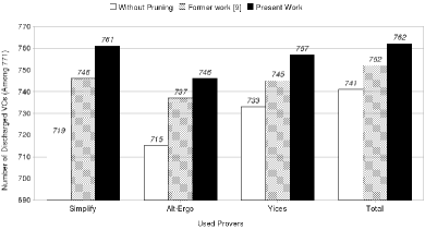
Figure 6: Result Comparison on Oslo Benchmark (771 VCs)

6.3 Public Why Benchmark

Our approach is developed in the Why tool, which translates Why syntax into the input syntax of several proof assistants (Coq, HOL 4, HOL Light, Isabelle/HOL, Mizar, PVS) and automated theorem provers (Alt-Ergo, CVC3, Simplify, Yices, Z3). This section shows some experimental results on the Why public benchmark.

The Why benchmark is a public collection of VCs generated by Caduceus or Krakatoa. These tools generate VCs respectively from C and Java programs, according to CSL and JML specifications. Hence, it partially matches to our requirements, since our work is focusing on the verification of VCs generated by these tools. The only limitation is that our method is focusing on VCs with a large amount of hypotheses, in contrast to the ones presented in this benchmark.

This benchmark is provided in two versions corresponding to two different pre-processes. Our results are similar with both versions. Alt-Ergo discharges 1260 VCs directly and 1297 VCs with axiom selection, while axiom selection adds 3 VCs to the 1310 VCs directly discharged by Simplify.

7 Related Work and Conclusion

We have presented a new strategy to select relevant hypotheses in formulae coming from program verification. To do so, we have combined two separate dependency analyses based on graph computation and graph traversal. Moreover, we have given some heuristics to analyse the graphs with a sufficient granularity. Finally we have shown the relevance of this approach with a benchmark issued from a real industrial code.

Strategies to simplify the prover’s task have been widely studied since automated provers exist [28], mainly to propose more efficient deductive systems [28, 27, 26]. The KeY deductive system [2] is an extreme case. It is composed of a large list of special purpose rules dedicated to JML-annotated JavaCard programs. These rules make unnecessary an explicit axiomatization of data types, memory model, and program execution. Priorities between deduction rules help in effective reasoning. Beyond this, choosing rules in that framework requires as much effort as choosing axioms when targeting general purpose theorem provers.

The present work can be compared with the set of support (sos) selection strategy [28, 20]. This approach starts with asking the user to provide an initial sos: it is classically the conclusion negation and a subset of hypotheses. It is then restricted to only apply inferences with at least one clause in the sos, consequences being added next into the sos. Our work can also be viewed as an automatic guess of the initial sos guided by the formula to prove. In this sense, it is close to [18] where initial relevant clauses are selected according to syntactical criteria, i.e. counting matching rates between symbols of any clause and symbols of clauses issued from the conclusion. By considering syntactical filtering on clauses issued from axioms and hypotheses, this latter work does not consider the relation between hypotheses, formalized by axioms of the theory: it provides a reduced forward proof. In contrast, by analyzing dependency graphs, we simulate natural deduction and are not far from backward proof search. By focusing on the predicative part of the verification condition, our objectives are dual to those developed in [14]: this work concerns boolean verification conditions with any boolean structure whereas we treat predicative formulae whose symbols are axiomatized in a quantified theory. Even in a large set of context axioms, most of the time, each verification condition only requires a tiny portion of this context. In [23, 7] a strategy to select relevant context axioms is presented, but it needs a preliminary manual task classifying axioms. Our predicate graph computation makes this axiom classification automatic. Recent advances have been made in the direction of semantic selection of axioms [25, 21]. Briefly speaking, at each iteration, the selection of each axiom depends on the fact whether a computed valuation is a model of the axiom or not. By comparison, our syntactical axiom selection is more efficient, indeed linear in the size of the input formula.

In a near future we plan to apply the strategy to other case studies. We also plan to investigate the impact on execution time of various strategies discharging the same list of verification conditions. We want to confirm or infirm with other benchmarks that weighting predicate dependencies with a formula length has no positive impact on automaticity but has a significant negative impact on the execution time. We also plan to integrate selection strategies in the Why tool or in a target automated theorem prover.

8 Acknowledgments

This work is partially funded by the French Ministry of Research, thanks to the CAT (C Analysis Toolbox) RNTL (Reseau National des Technologies Logicielles), by the SYSTEM@TIC Paris Region French cluster, thanks to the PFC project (Plateforme de Confiance, trusted platforms), and by the INRIA, thanks to the CASSIS project and the CeProMi ARC. The authors also want to thank Christophe Ringeissen and the four anonymous referees for their insightful comments.

References

- [1] M. Barnett, K. R. M. Leino, and W. Schulte. The Spec# Programming System: An Overview. In Construction and Analysis of Safe, Secure, and Interoperable Smart Devices (CASSIS’04), volume 3362 of Lecture Notes in Computer Science, pages 49–69. Springer, 2004.
- [2] B. Beckert, R. Hähnle, and P. H. Schmitt, editors. Verification of Object-Oriented Software: The KeY Approach. LNCS 4334. Springer-Verlag, 2007.
- [3] Bernhard Kauer. OSLO: Improving the security of Trusted Computing. In 16th USENIX Security Symposium, August 6-10, 2007, Boston, MA, USA, 2007.
- [4] L. Burdy, Y. Cheon, D. Cok, M. Ernst, J. Kiniry, G. T. Leavens, K. R. M. Leino, and E. Poll. An overview of JML tools and applications. Technical Report NIII-R0309, Dept. of Computer Science, University of Nijmegen, 2003.
- [5] J.-F. Couchot and T. Hubert. A Graph-based Strategy for the Selection of Hypotheses. In FTP 2007 - International Workshop on First-Order Theorem Proving, Liverpool, UK, Sept. 2007.
- [6] L. M. de Moura, B. Dutertre, and N. Shankar. A tutorial on satisfiability modulo theories. In W. Damm and H. Hermanns, editors, CAV, volume 4590 of Lecture Notes in Computer Science, pages 20–36. Springer, 2007.
- [7] D. Deharbe and S. Ranise. Satisfiability Solving for Software Verification. Submitted in 2006. See http://www.loria.fr/~ranise/pubs/sttt-submitted.pdf.
- [8] E. Denney, B. Fischer, and J. Schumann. An empirical evaluation of automated theorem provers in software certification. International Journal on Artificial Intelligence Tools, 15(1):81–108, 2006.
- [9] D. Detlefs, G. Nelson, and J. B. Saxe. Simplify: a theorem prover for program checking. J. ACM, 52(3):365–473, 2005.
- [10] D. L. Detlefs, K. R. M. Leino, G. Nelson, and J. B. Saxe. Extended static checking. Technical Report 159, Compaq Systems Research Center, Dec. 1998. Available at http://www.hpl.hp.com/techreports/Compaq-DEC/SRC-RR-159.html.
- [11] E. W. Dijkstra. A discipline of programming. Series in Automatic Computation. Prentice Hall Int., 1976.
- [12] J.-C. Filliâtre and C. Marché. The Why/Krakatoa/Caduceus platform for deductive program verification. In 19th International Conference on Computer Aided Verification, volume 4590 of \balancecolumnsLecture Notes in Computer Science, pages 173–177. Springer, 2007.
- [13] A. Giorgetti and J. Groslambert. JAG: JML Annotation Generation for Verifying Temporal Properties. In Luciano Baresi and Reiko Heckel, editors, Fundamental Approaches to Software Engineering, 9th International Conference, FASE 2006, volume 3922 of Lecture Notes in Computer Science, pages 373–376. Springer, 2006.
- [14] E. P. Gribomont. Simplification of boolean verification conditions. Theoretical Computer Science, 239(1):165–185, 2000.
- [15] J. Groslambert and N. Stouls. Vérification de propriétés LTL sur des programmes C par génération d’annotations. In AFADL’09, 2009. Short paper.
- [16] T. Hubert and C. Marché. Separation analysis for deductive verification. In Heap Analysis and Verification (HAV’07), Braga, Portugal, Mar. 2007.
- [17] K. R. M. Leino. Efficient weakest preconditions. Information Processing Letters, 93(6):281–288, 2005.
- [18] J. Meng and L. Paulson. Lightweight relevance filtering for machine-generated resolution problems. In ESCoR: Empirically Successful Computerized Reasoning, 2006.
- [19] A. Nonnengart and C. Weidenbach. Computing Small Clause Normal Forms. In A. Robinson and A. Voronkov, editors, Handbook of Automated Reasoning, volume I, chapter 6, pages 335–367. Elsevier Science, 2001.
- [20] D. A. Plaisted and A. H. Yahya. A relevance restriction strategy for automated deduction. Artificial Intelligence, 144(1-2):59–93, 2003.
- [21] P. Pudlak. Semantic selection of premisses for automated theorem proving. In G. Sutcliffe, J. Urban, and S. Schulz, editors, CEUR Workshop Proceedings, volume 257, pages 27–44, 2007.
- [22] S. Ranise and C. Tinelli. The Satisfiability Modulo Theories Library (SMT-LIB). http://www.SMT-LIB.org, 2006.
- [23] W. Reif and G. Schellhorn. Theorem proving in large theories. In M. P. Bonacina and U. Furbach, editors, Int. Workshop on First-Order Theorem Proving, FTP’97, pages 119–124. Johannes Kepler Universität, Linz (Austria), 1997.
- [24] N. Stouls. Hypotheses selection applied to trusted computing. http://perso.citi.insa-lyon.fr/nstouls/tools/oslo/.
- [25] G. Sutcliffe and Y. Puzis. Srass - a semantic relevance axiom selection system. In Springer, editor, Automated Deduction - CADE-21, 21st International Conference on Automated Deduction, Bremen, Germany, July 17-20, 2007, Proceedings, volume 4603 of Lecture Notes in Computer Science, pages 295–310, 2007.
- [26] L. Wos. Conquering the meredith single axiom. Journal of Automated Reasoning, 27(2):175–199, 2001.
- [27] L. Wos and G. W. Pieper. The hot list strategy. Journal of Automated Reasoning, 22(1):1–44, 1999.
- [28] L. Wos, G. A. Robinson, and D. F. Carson. Efficiency and completeness of the set of support strategy in theorem proving. J. ACM, 12(4):536–541, 1965.