New dynamical pair breaking effect

Abstract

A dynamical pair breaking effect is evidenced at very low excitation energies. For this purpose, a new set of time-dependent coupled channel equations for pair-breaking in superfluid systems are deduced from the variational principle. These equations give the probability to destroy or to create a Cooper pair under the action of some perturbations or when the mean field varies in time. The odd-even effect in fission is investigated within the model as an example. For this purpose, the time-dependent probability to find the system in a seniority-one or in a seniority-two state is restricted in the sense that the perturbations are considered only in the avoided crossing regions.

1 Introduction

In atomic or nuclear molecules, fermions move in a common field generated by several centers of force. The potential depends on the so-called generalized coordinates. The most used generalized variables are function of the inter-nuclear distances and their angular dependencies. In such a molecular description, the motion of the nuclear centers is considered adiabatically slow compared with the rearrangement of the mean field. The atoms or the nuclei share their valence electrons and their outer-bound nucleons, respectively. Enhancements and structures in the energy dependence of the cross section in atomic [1, 2] and nuclear [3, 4] reactions reflect a special signature of the presence of molecular orbitals. The behavior of the cross section is usually explained in terms of the Landau-Zener effect.

The Landau-Zener effect [5, 6] describes the non-adiabatic transitions at avoided crossing regions between potential curves [7, 8] or energy levels [9, 10]. Two levels with the same good quantum numbers associated to some symmetries cannot intersect and exhibit avoided level crossing regions. A small perturbation energy is always available in these regions, being responsible for the level slippage mechanism. Recently, the time-dependent equations that describe quantitatively the Landau-Zener promotion mechanism were generalized for molecular potentials that include pairing residual interactions [11]. As evidenced below, this generalization also provides a way to formulate a theory for a new dynamical pair breaking mechanism. Originally, the pairing formalism, reflected in the BCS equations, was used to explain superconducting states in terms of two electrons pairs with opposite momenta and spin near the Fermi surface [12].

2 Formalism

The dynamical pair breaking effect emerges from a new set of coupled channel equations deduced for the time-dependent probability to find the system in a seniority-one state or in a seniority-two one. The variation of the mean field is considered slow enough, so that fermions follow eigenstates of the instantaneous mean field. In such an approximation, if the interactions produced in the avoided crossing regions or those due to the Coriolis coupling are not taken into consideration, other perturbations between two different states are not possible. In the following, the calculations are restricted only for perturbations produced in the avoided crossing regions. This approximation does not affect the essential features of the model but leads to a considerable simplification of the mathematical apparatus.

The starting point is a many-body Hamiltonian with pairing residual interactions. This Hamiltonian depends on some time-dependent collective parameters $q(t)=\{q_{i}(t)\}$ ($i=1,...n$), such as the internuclear distances between atoms or nuclei:

$$H(t)=\sum_{k>0}\epsilon_{k}[q(t)](a_{k}^{+}a_{k}+a_{\bar{k}}^{+}a_{\bar{k}})-G\sum_{k,i>0}a_{k}^{+}a_{\bar{k}}^{+}a_{i}a_{\bar{i}}.$$ (1)

Here, $\epsilon_{k}$ are single-particle energies of the molecular potential, $a_{k}^{+}$ and $a_{k}$ denote operators for creating and destroying a particle in the state $k$, respectively. The state characterized by a bar signifies the time-reversed partner of a pair. The pairing correlation arise from the short range interaction between fermions moving in time-reversed orbits. The essential feature of the pairing correction can be described in terms of a constant pairing interaction $G$ acting between a given number of particles. In this paper, the sum over pairs generally runs over the index $k$. Because the pairing equations diverge for an infinite number of levels, a limited number of levels are used in the calculation, that is $N$ levels above and below the Fermi energy $E_{F}$.

Using quasiparticle creation and annihilation operators

$$\alpha_{k(\gamma)} = u_{k(\gamma)}a_{k}-v_{k(\gamma)}a_{\bar{k}}^{+};$$

$$\alpha_{\bar{k}(\gamma)} = u_{k(\gamma)}a_{\bar{k}}+v_{k(\gamma)}a_{k}^{+};$$ (2)

$$\alpha_{k(\gamma)}^{+} = u_{k(\gamma)}a_{k}^{+}-v_{k(\gamma)}^{*}a_{\bar{k}};$$

$$\alpha_{\bar{k}(\gamma)}^{+} = u_{k(\gamma)}a_{\bar{k}}^{+}+v_{k(\gamma)}^{*}a_{k};$$

it is possible to construct some interactions able to break a Cooper pair when the system traverses a avoided crossing region. The parameters $v_{k(\gamma)}$ and $u_{k(\gamma)}$ are occupation and vacancy amplitudes, respectively, for a pair occupying the single-particle level $k$ of the configuration $(\gamma)$. The seniority-zero configuration is labeled with $(\gamma)=(0)$ and the seniority-two configuration by a pair of indexes denoting the levels blocked by the unpaired fermions $(\gamma)=(ij)$. The three situations plotted in Fig. 1 can be modeled within products of such creation and annihilation operators acting on Bogoliubov wave functions. In the plot 1(a), the Cooper pairs remain on the adiabatic levels $\epsilon_{i}$ and $\epsilon_{j}$ after the passage through the avoided crossing region, in Fig. 1 (b) the pair destruction is illustrated, while in Fig. 1 (c) two fermions generate a pair after the passage through an avoided crossing region. Formally, to describe these three situations, an interaction in the avoided crossing can be postulated as follows:

$$H^{\prime}(t) = \sum_{i,j\neq i}^{n}h_{ij}[q(t)]\left[\alpha_{i(0)}\alpha_{\bar{j}(0)}\prod_{k\neq i,j}\alpha_{k(0)}a_{k}^{+}a_{k}\alpha_{k(ij)}^{+}\right.$$ (3)

$$\left.+\alpha_{i(0)}^{+}\alpha_{\bar{j}(0)}^{+}\prod_{k\neq i,j}\alpha_{k(ij)}a_{k}^{+}a_{k}\alpha_{k(0)}^{+}\right],$$

where $h_{ij}$ is the interaction between the levels. The form of the perturbation (3) was postulated in Ref. [11] and was successfully used to generalize the Landau-Zener effect in seniority-one superfluid systems. Acting on a suited Bogoliubov wave function, the product over $k$ transforms the seniority-two configuration in the seniority-zero one in the case of the first term in the left hand of Eq. (3), and vice-versa in the case of the second term. If the product $\alpha_{i(0)}\alpha_{\bar{j}(0)}$ acts on a seniority-zero function, then it annihilates a pair and creates two unpaired fermions in states $i$ and $\bar{j}$. If the product $\alpha_{i(0)}^{+}\alpha_{\bar{j}(0)}^{+}$ acts on a seniority-two wave function, then it creates a pair distributed on both orbitals $i$ and $j$. In order to obtain the equations of motion, we shall start from the variational principle taking the following energy functional

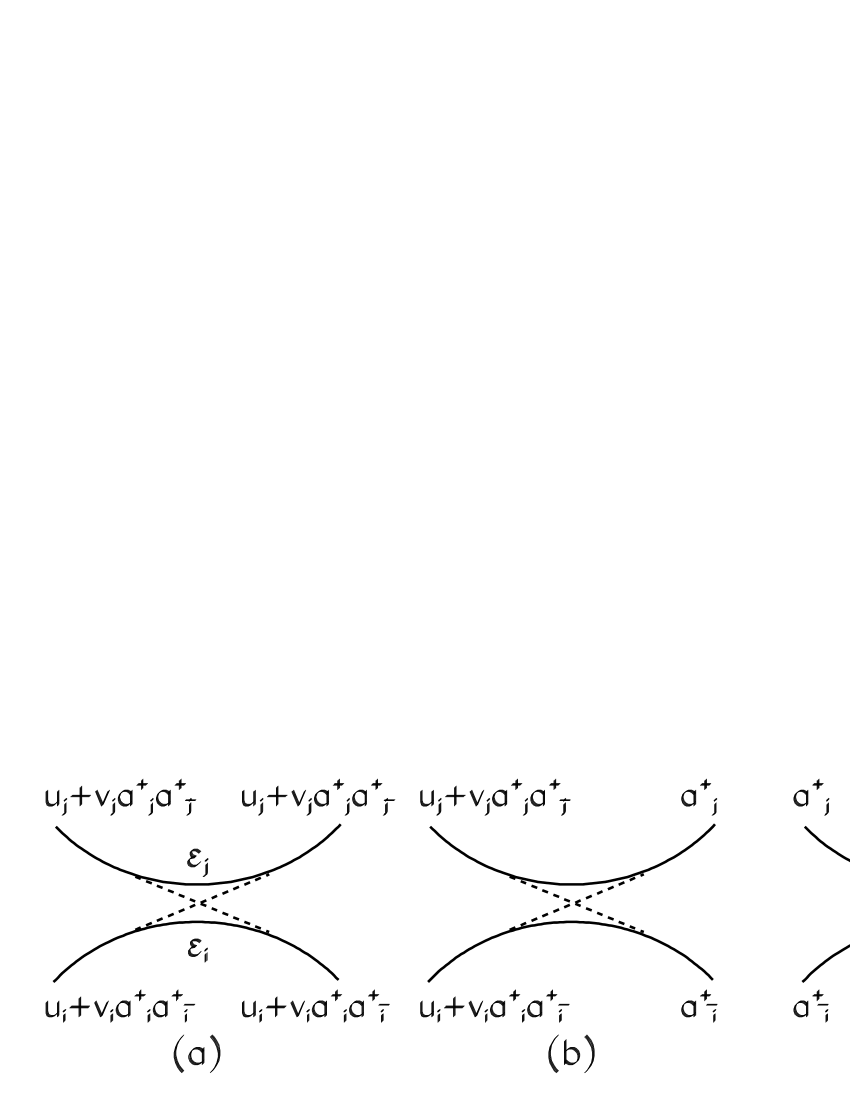
Figure 1: Ideal avoided crossing regions between two adiabatic levels $\epsilon_{i}$ and $\epsilon_{j}$. Three possible transitions between configurations in an avoided crossing region in the superfluid model are displayed: (a) The configuration remains unchanged after the passage through the avoided crossing region. (b) A pair is broken. (c) A pair is created.

$${\cal{L}}=<\varphi\mid H-i\hbar{\partial\over\partial t}+H^{\prime}-\lambda\hat{N}\mid\varphi>$$ (4)

and by assuming the many-body state formally expanded as a superposition of time dependent BCS seniority-zero and seniority-two adiabatic wave functions

$$\mid\varphi(t)> = \left[c_{0}(t)\prod_{k}\left(u_{k(0)}(t)+v_{k(0)}(t)a_{k}^{+}a_{\bar{k}}^{+}\right)\right.$$

$$+\sum_{j,l\neq j}c_{jl}(t)a_{j}^{+}a_{\bar{l}}^{+}$$

$$\left.\times\prod_{k\neq j,l}\left(u_{k(jl)}(t)+v_{k(jl)}(t)a_{k}^{+}a_{\bar{k}}^{+}\right)\right]\mid 0>,$$

where $c_{0}$ and $c_{jl}$ are amplitudes of the two kind of configurations. Here, $\lambda$ is the chemical potential, and $\hat{N}$ is the particle number operator. To minimize this functional, the expression (4) is derived with respect the independent variables $v_{k(0)}$, $v_{k(jl)}$, $c_{0}$, $c_{jl}$, together with their complex conjugates, and the resulting equations are set to zero. Eventually, eight coupled-channel equations are obtained:

$$i\hbar\dot{\rho}_{k(0)} = \kappa_{k(0)}\Delta_{0}^{*}-\kappa_{k(0)}^{*}\Delta_{0};$$

$$i\hbar\dot{\rho}_{k(jl)} = \kappa_{k(jl)}\Delta_{jl}^{*}-\kappa_{k(jl)}^{*}\Delta_{jl};$$

$$i\hbar\dot{\kappa}_{k(0)} = \left(2\rho_{k(0)}-1\right)\Delta_{0}+2\kappa_{k(0)}\left(\epsilon_{k}-\lambda_{0}\right)$$

$$-2G\rho_{k(0)}\kappa_{k(0)};$$

$$i\hbar\dot{\kappa}_{k(jl)} = \left(2\rho_{k(jl)}-1\right)\Delta_{jl}+2\kappa_{k(jl)}\left(\epsilon_{k}-\lambda_{jl}\right)$$

$$-2G\rho_{k(jl)}\kappa_{k(jl)};$$

$$i\hbar\dot{P}_{0} = \sum_{l,j\neq l}h_{jl}(S_{0jl}^{*}-S_{0jl});$$ (6)

$$i\hbar\dot{P}_{jl} = h_{jl}(S_{0jl}-S_{0jl}^{*});$$

$$i\hbar\dot{S}_{0jl} = S_{0jl}(E_{0}-N\lambda_{0}-E_{jl}+N\lambda_{jl})$$

$$+S_{0jl}\left(\sum_{k\neq j,l}T_{k(jl)}-\sum_{k}T_{k(0)}\right)$$

$$+\sum_{m,n\neq m}h_{mn}S_{mnjl}+h_{jl}(P_{jl}-P_{0});$$

$$i\hbar\dot{S}_{mnjl} = S_{mnjl}(E_{mn}-N\lambda_{mn}-E_{jl}+N\lambda_{jl})$$

$$+S_{mnjl}\left(\sum_{k\neq m,n}T_{k(mn)}-\sum_{k\neq j,l}T_{k(jl)}\right)$$

$$+h_{mn}S_{0jl}-h_{jl}S_{0mn}^{*};$$

where the partial derivatives with respect the time are denoted by a dot. The sums are restricted by the conditions $j\neq l$, $m\neq n$, $m\neq j$, and $n\neq l$. $E_{\gamma}$ are exactly the expected values of the Hamiltonian (1) for the seniority-zero or seniority-two configurations:

$$E_{0} = 2\sum_{k}\rho_{k(0)}\epsilon_{k}-{\mid\Delta_{0}\mid^{2}\over G}-G\sum_{k}\rho_{k(0)}^{2};$$

$$E_{jl} = 2\sum_{k\neq j,l}\rho_{k(jl)}\epsilon_{k}-{\mid\Delta_{jl}\mid^{2}\over G}$$ (7)

$$-G\sum_{k\neq j,l}\rho_{k(jl)}^{2}+\epsilon_{j}+\epsilon_{l};$$

and $T_{k(\gamma)}$ are energy terms associated to single-particle states:

$$T_{k(\gamma)} = 2\rho_{k(\gamma)}(\epsilon_{k}-\lambda_{\gamma})-2G\rho_{k(\gamma)}^{2}$$

$$+{\kappa_{k(\gamma)}\Delta_{\gamma}^{*}+\kappa_{k(\gamma)}^{*}\Delta_{\gamma}\over 2}\left({\rho_{k(\gamma)}^{2}\over\mid\kappa_{k(\gamma)}\mid^{2}}-1\right).$$

The following notations are used in Eqs. (6):

$$\Delta_{0} = G\sum_{k}\kappa_{k(0)};$$

$$\Delta_{jl} = G\sum_{k\neq j,l}\kappa_{k(jl)};$$

$$\kappa_{k(\gamma)} = u_{k(\gamma)}v_{k(\gamma)};$$

$$\rho_{k(\gamma)} = \mid v_{k(\gamma)}\mid^{2};$$ (8)

$$P_{\gamma} = \mid c_{\gamma}\mid^{2};$$

$$S_{\gamma\gamma^{\prime}} = c_{\gamma}c_{\gamma^{\prime}}^{*};$$

where $\rho_{k(\gamma)}$ are single-particle densities and $\kappa_{k(\gamma)}$ are pairing moment components. $P_{\gamma}$ denote the probabilities to find the system in the configurations $\gamma$. $S_{\gamma\gamma^{\prime}}$ are moment components between two configurations $\gamma$ and $\gamma^{\prime}$ and have the property $\mid S_{\gamma\gamma^{\prime}}\mid^{2}=P_{\gamma}P_{\gamma^{\prime}}$. $\Delta_{\gamma}$ is the gap parameter. The values of $\rho_{k(\gamma)}$ and $P_{\gamma}$ are reals. The particle number conservation conditions $2\sum_{k}\rho_{k(0)}=2N$, $2\sum_{k\neq j,l}\rho_{k(jl)}=2N-2$ and $P_{0}+\sum_{j,l\neq j}P_{jl}=1$ are fulfilled by Eqs. (6).

3 Application to fission processes

A direct application of the system (6) is related to the pair breaking and the odd-even structure in fission fragment yields. In fission, it is considered that the paired configuration is preserved until an interaction breaks some pairs in combination with the existence of a sufficient high excitation energy. The odd-even structure in fission is explained usually within statistical arguments, as for example in Refs. [13, 14]. Alternatively, the probability to break a pair can be determined dynamically by taking into account only the interaction available in the avoided crossing regions within the present model.

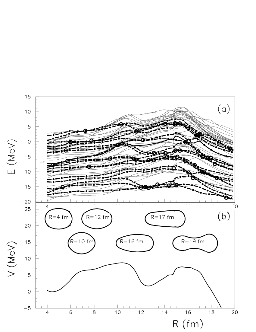
Figure 2: (a) Proton level scheme as function of the inter-nuclear distance $R$ between the nascent fragments along the minimal action path for the ²³⁴U fission. Only $N$=60 single-particle energies above and below the Fermi level are plotted. The Fermi level $E_{F}$ is displayed with a thick full curve. The selected $\Omega$=1/2 levels ($\epsilon_{1},...\epsilon_{17}$) are plotted with thick dot-dashed lines. Avoided level crossing regions are marked with circles. The maximum number of major shells used in calculations is 12. (b) The fission barrier as function of the internuclear distance $R$. Nuclear shapes corresponding to several special configurations are inserted in the plot. The values of the internuclear distances are also marked. At $R\approx 4$ fm, the ground-state configuration of the parent is found.

To solve the pair breaking equations (6), the variations of single-particle energies $\epsilon_{k}$ together with perturbations $h_{ij}$ must be supplied. The simplest way to obtain these evolutions is to consider a time-dependent mean field in which the nucleons move independently. In most usual treatments of nuclear fission, the whole nuclear system is characterized by some collective variables, which determine approximately the behavior of many other intrinsic variables. The generalized coordinates vary in time leading to a split of the nuclear system. The basic ingredient in such an analysis is a nuclear shape parametrization. In the following treatment, a nuclear shape parametrization is given by two ellipsoids of different sizes smoothly joined by a third surface obtained [11] by the rotation of a circle around the axis of symmetry. Five degrees of freedom characterize this parametrization: the elongation given by the inter-nuclear distance $R$ between the centers of the ellipsoids, the two deformations of the nascent fragments, the mass asymmetry and the necking parameter. Due to the axial symmetry, the good quantum numbers are the projections of the intrinsic spin $\Omega$.

As specified in Ref. [15], first of all, a calculation of the fission trajectory in our five-dimensional configuration space, beginning with the ground-state of the system up to the exit point of the barrier must be performed. This can be done by minimizing the action integral. For this purpose, two ingredients are required: the deformation energy $V$ and the tensor of the effective mass. The deformation energy was obtained in the frame of the microscopic-macroscopic method [16] by summing the liquid drop energy with the shell and the pairing corrections. The macroscopic energy is obtained in the framework of the Yukawa plus exponential model [17] extended for binary systems with different charge densities [18]. The Strutinsky microscopic corrections were computed on the basis of the Woods-Saxon superasymmetric two center shell model. The effective mass is computed within the cranking approximation [19]. After minimization, the dependences between the generalized coordinates $q_{i}$ ($i=1,...5$) in the region comprised between the parent ground state configuration and the exit point of the external fission barrier supply the least action trajectory. The ground-state corresponds to the lowest deformation energy in the first well. The least action trajectory is obtained within a numerical method. Details about the numerical procedure of minimization and about the model can be found in Refs. [10, 11] and references therein. The resulting ²³⁴U fission barrier is plotted on Fig. 2 (b) as function of the distance between the centers of the nascent fragments $R$. Some nuclear shapes obtained along the minimal action trajectory are inserted in the plot. A realistic proton level scheme along the least action trajectory is obtained within the superasymmetric Woods-Saxon two-center shell model [11]. This model gives the single particle level diagrams by diagonalizing a Woods-Saxon potential, corrected within spin-orbit and Coulomb terms, in the analytic eigenvalue basis of the two center semi-symmetric harmonic model [20, 21]. Other recipes to obtain the level scheme are related to the molecular orbital method [22]. The proton level scheme is displayed in Fig. 2 (a).

Figure 3: (a) The average excitation energy $E^{*}$ as function of the elongation $R$. The inter-nuclear velocities $\dot{R}$ are 10⁴, 10⁵ and 10⁶ m/s for the dashed, full and dot-dashed lines, respectively. (b) The probability $P_{odd}$ of a seniority-two state with respect to the elongation $R$. The same line types and inter-nuclear velocities as in panel (a) are used. (c) The probabilities to obtain a seniority-zero state $P_{0}$ and a seniority-two state $P_{odd}$ as function of the excitation energy $E^{*}$ of the fragments at the elongation $R$=20 fm.

The Landau-Zener effect is produced only in the workspace spanned by levels characterized by the same good quantum numbers. As mentionned, due to the axial symmetry, the good quantum numbers are the projections of the intrinsic spin $\Omega$. Therefore, among the $N$ states in the region near the Fermi surface, the 17 levels with spin projection $\Omega$=1/2 are selected. These levels are plotted with thick dot-dashed lines in Fig. 2 (a). Because a pair creation or annihilation is considered to be possible only between adjacent levels, 16 seniority-two configurations are constructed. The initial values of quantities(8) are obtained by solving the BCS equations for the ground states of all $\gamma$ configurations. The average excitation energy of the seniority-zero state is computed as in Ref. [23, 24] with the relation $E^{*}=(E_{0}-E_{0}^{0})+E_{n}^{*}$, where $E_{0}^{0}$ is the value of the lowest energy state of any deformation calculated within the BCS approach and $E_{0}$ is obtained with Eqs. (7). Here, $E_{n}^{*}$ is the dissipation obtained within the same formalism for the even neutron subsystem. The probability to obtain a seniority-two state is simply $P_{odd}=1-P_{0}$. The values of $E^{*}$ and $P_{odd}$ are plotted in Fig. 3 (a) and (b) as function of the elongation for some inter-nuclear velocities $\dot{R}$. In connection with the shape of the barrier displayed in Fig. 2, it can be deduced that the larger part of the odd-even yield is formed during the penetration of the second barrier and the excitation energy increases merely in the same region. Different constant values of the inter-nuclear velocity $\dot{R}$ ranging from 10⁴ to 10⁶ m/s were tested. These values can be translated in a time to penetrate the barrier ranging in the interval $[1.4\times 10^{-18},1.4\times 10^{-20}]$ s. In Fig. 3 (c), the dependences of $P_{0}$ and $P_{odd}$ versus $E^{*}$ are displayed in the selected velocity domain. The results exhibit a clear decrease of $P_{odd}$ as function of $E^{*}$. It is interesting to note that at zero excitation energy, the probability to find the system in a seniority-two state is practically one. In cold fission, at very low excitation energies of the fragments, the odd-even yields are always larger than the even-even ones [25, 26, 27]. The even-even fragmentation dominates at larger excitation energies of the fragments, above 4-6 MeV. It is a very strange phenomenon because in cold processes the system doesn’t possess enough energy to break a pair and because the penetrability is hindered for odd-systems due to the specialization energies associated to the two unpaired nucleons. Up to now, the statistical explanation of this phenomenon involved some modifications of the level densities for odd-even and even-even partitions [14] by according them within the deformations of the fragments as function of the excitation energies and the shell effects. However, if one assumes that the odd-even effect in the fission fragments distribution is strongly correlated to the seniority-two state probability, this phenomenon can be alternatively explained by solving the coupled-channel system of time-dependent pair breaking equations as evidenced above. In this work, only the $\Omega$=1/2 subspace of the proton level diagram is treated, but the same formalism can be applied to other subspaces.

In conclusion, a new set of time-dependent coupled channel equations derived from the variational principle is proposed to determine dynamically the mixing between seniority-zero and seniority-two configurations. The essential idea is that the configuration mixing is managed under the action of some inherent low lying time dependent excitations produced in the avoided crossing regions. These equations were used to explain the odd-even effect in cold fission processes. Only the radial coupling was used in the analysis, but it is possible to extend the equations to take into account even the Coriolis coupling, as in Ref. [28]. The main trends concerning the dependence of the odd-even effect in fragments yields versus the fragments excitation energy were reproduced. The formalism can be adjusted for other types of processes. In this respect, the value of the interaction $h_{\gamma\gamma^{\prime}}$ can also be the magnitude of other kind of interactions between different configurations and the collective variables could be the amplitude of an external applied field as encountered in the field of condensed matter. The essential idea is the inclusion in the energy functional of a time dependent low perturbation by the mean of quasiparticle operators.

Acknowledgments This work was supported by the CNCSIS IDEI 512 contract of the Romanian Ministry of Education and Research.

References

- [1] U. Fano and W. Lichten, Phys. Rev. Lett. 14 (1965) 627.
- [2] W. Lichten, Phys. Rev. 164 (1967) 131.
- [3] B. Milek and R. Reif, Phys. Lett. B 157 (1985) 134.
- [4] J.Y. Park, W. Greiner and W. Scheid, Phys. Rev. C 21 (1980) 958.
- [5] L.D. Landau, Phys. Z. Sowjetunion 2 (1932) 46.
- [6] C. Zener, Proc. Roy. Soc. A 137 (1932) 696.
- [7] R.A. Marcus, Rev. Mod. Phys. 65 (1993) 599.
- [8] N. Bohr and J. Wheeler, Phys. Rev. 16 (1939) 426.
- [9] J.R. Rubbmark, M.M. Kash, M.G. Littman, and D. Kleppner, Phys. Rev. A 23 (1981) 3107.
- [10] M. Mirea, L. Tassan-Got, C. Stephan, C.O. Bacri, and R.C. Bobule scu, Phys. Rev. C 76 (2007) 064608.
- [11] M. Mirea, Phys. Rev. C 78 (2008) 044618.
- [12] J. Bardeen, L.N. Cooper, and J.R. Schrieffer, Phys. Rev. 108 (1957) 1175.
- [13] F. Rejmund, A.V. Ignatyuk, A.R. Junghans, and K.-H. Schmidt, Nucl Phys. A 678 (2000) 215.
- [14] V. Avrigeanu, A. Florescu, A. Sandulescu, and W. Greiner, Phys. Rev. C 52 (1995) R1755.
- [15] M. Brack, J. Damgaard, A.S. Jensen, H.C. Pauli, V.M. Strutinsky, and C.Y. Wong, Rev. Mod. Phys. 44 (1972) 320.
- [16] J.R. Nix, Ann. Rev. Nucl. Sci. 22 (1972) 65.
- [17] K.T.R. Davies, and J.R. Nix, Phys. Rev. C 14 (1976) 1977.
- [18] M. Mirea, O. Bajeat, F. Clapier, F. Ibrahim, A.C. Mueller, N. Pauwels, and J. Proust, Europ. Phys. J. A 11 (2001) 59.
- [19] M. Mirea, R.C. Bobulescu, and M. Petre, Rom. Rep. Phys., in print .
- [20] M. Mirea, Nucl. Phys. A 780 (2006) 13.
- [21] J. Maruhn, and W. Greiner, Z. Phys. 251 (1972) 431.
- [22] A. Diaz-Torres, Phys. Rev. Lett. 101 (2008) 122501.
- [23] M. Mirea, L. Tassan-Got, C. Stephan, and C.O. Bacri, Nucl. Phys. A 735 (2004) 21.
- [24] S.E. Koonin, and J.R. Nix, Phys. Rev. C 13 (1976) 209.
- [25] H.-G. Clerc, in Heavy Elements and Related New Phenomena, edited by W. Greiner and R.K. Gupta (World Scientific, 1999), p. 451.
- [26] W. Schwab, H.-G. Clerc, M. Mutterer, J.P. Theobald, and H. Faust, Nucl. Phys. A 577 (1994) 674.
- [27] F.-J. Hambsch, H.-H. Knitter, and C. Budtz-Jorgensen, Nucl. Phys. A 554 (1993) 209.
- [28] M. Mirea, Phys. Rev. C 63 (2001) 034603.