Ferro-Nematic ground state of the dilute dipolar Fermi gas

Abstract

It is shown that a homogeneous two-component Fermi gas with (long range) dipolar and short-range isotropic interactions has a ferro-nematic phase for suitable values of the dipolar and short-range coupling constants. The ferro-nematic phase is characterized by having a non-zero magnetization and long range orientational uniaxial order. The Fermi surface of spin up (down) component is elongated (compressed) along the direction of the magnetization.

Cold dipolar Fermi gases have attracted much attention due to the novel anisotropic and long-range character of dipole-dipole interactions. Recent studies of many-body effects predicted an elongated Fermi surface (FS) in a one-component fully polarized Fermi gas with dipolar interactions along the polarization direction established by an external fieldMiyakawa et al. (2008); Sogo et al. (2009). A biaxial state with a critical value of the effective coupling constant $\lambda_{d}=n\mu^{2}/\epsilon_{F}$ was proposed in Ref. Fregoso et al. (2009) ($\mu$ is the dipole moment of the fermion, $n$ is the total density and $\epsilon_{F}$ is the Fermi energy of the free Fermi gas at the same density). It was foundFregoso et al. (2009) that the system will exhibit violations of the Landau theory of the Fermi liquid both at quantum criticality and in the biaxial phase. More generally, understanding anisotropic non-Fermi liquid phases of cold atomic systems may shed light into the quantum liquid crystal phases in strongly correlated systems and high $T_{c}$ superconductors Kivelson et al. (1998); Oganesyan et al. (2001); Sun et al. (2008).

The question we want to address here is whether a cold spin-$\nicefrac{{1}}{{2}}$ Fermi gas with long range dipolar interactions can become spontaneously polarized and what is the nature of the broken symmetry state. The theory we present here is a generalization of the theory of the Stoner (ferromagnetic) transition in metalsDoniach and Sondheimer (1998) to take into account the effects of the long range and anisotropic dipolar interactionmah . As we will see below, much as in the theory of Stoner ferromagnetism, the polarized state can occur only for sufficiently large values of the magnetic dipole moment and/or of the spin-flip scattering rate. However, unlike what happens in Stoner ferromagnetism, as a result of the structure of the dipolar interactions, the resulting polarized state is also spatially anisotropic, a ferro-nematic state.

The classical version of this problem has been considered in mixtures of ferromagnetic particles with nematic liquid crystalsBrochard and de Gennes (1970), and in dipolar colloidal fluids and ferrofluidsSeul and Andelman (1995). Classical dipolar fluids have complex phase diagrams, typically featuring inhomogeneous phases with complex spatial structures. Much less is known about their quantum counterparts. In the case of simple quantum fluids, such as ³He, the dipolar interaction plays a small role compared to the short-range exchange interactionFomin et al. (1978). In the context of ultracold gases, a number of atomic and molecular systems with strong dipolar interactions, such as Dy, have been the focus of recent experiments (see Ref.Leefer et al. (2009)).

Consider a restricted Hilbert space of two hyperfine states, called $1$ (“spin up”) and $2$ (“spin down”), of a point-like magnetic atom of mass $m$ and magnetic moment, $\mathbf{M}$, with components $M_{i}=\mu\sigma^{i}$ ($i=1,2,3$) and $\vec{\sigma}$ are the usual spin-$\nicefrac{{1}}{{2}}$ Pauli matrices (the factor of $\hbar/2$ is absorbed in the definition of $\mu$). The Hamiltonian is

$$\hat{H} = \int d^{3}x\psi_{\alpha}^{\dagger}(\mathbf{x})\left(-\frac{\hbar^{2}\nabla^{2}}{2m}\right)\psi_{\alpha}(\mathbf{x})+\frac{1}{2}\int d^{3}xd^{3}x^{\prime}$$ (1)

$$\times\psi_{\alpha}^{\dagger}(\mathbf{x})\psi_{\beta}^{\dagger}(\mathbf{x}^{\prime})U_{0}(\mathbf{x},\mathbf{x}^{\prime})_{\alpha\alpha^{\prime};\beta\beta^{\prime}}\psi_{\beta^{\prime}}(\mathbf{x}^{\prime})\psi_{\alpha^{\prime}}(\mathbf{x})$$

where the fields $\psi_{\alpha}(\mathbf{x})$ destroy fermions on spin state with $z$-component $\alpha=1,2$ at position $\mathbf{x}$. We consider the model interaction is of the form

$$U_{0}(\mathbf{x},\mathbf{x}^{\prime})_{\alpha\alpha^{\prime};\beta\beta^{\prime}} = \frac{\mu^{2}}{r^{3}}\sigma^{i}_{\alpha\alpha^{\prime}}(\delta_{ij}-3\mathbf{\hat{r}}_{i}\mathbf{\hat{r}}_{j})\sigma^{j}_{\beta\beta^{\prime}}$$ (2)

$$\hskip 20.0pt+\hskip 2.0ptg\hskip 2.0pt\delta_{\alpha\alpha^{\prime}}\delta_{\beta\beta^{\prime}}\delta(\mathbf{r})$$

where $\mathbf{r}\equiv(\mathbf{x}-\mathbf{x}^{\prime})/|\mathbf{x}-\mathbf{x}^{\prime}|$ and $\mathbf{\hat{r}}$ is a unit vector in the direction of $\mathbf{r}$. The last (ultra-local) term represents the short-range isotropic (contact) interactions. It only affects the spin-triplet channel and we denote by $g$ the associated coupling constant. The Fourier transform of the bare two body interaction is $(4\pi\mu^{2}/3)\sigma^{i}_{\alpha\alpha^{\prime}}(3\mathbf{\hat{q}}_{i}\mathbf{\hat{q}}_{j}-\delta_{ij})\sigma^{j}_{\beta\beta^{\prime}}+g\delta_{\alpha\alpha^{\prime}}\delta_{\beta\beta^{\prime}}$. The Hamiltonian is invariant under simultaneous $SU(2)$ transformations in spin space and $SO(3)$ rotations in real space. This mixing of orbital and spin degrees of freedom is, in essence, what relates the distortions of the shape of FS and the spin polarization.

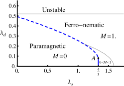
Figure 1: (color online) Schematic phase diagram as a function of $\lambda_{s}=gn/\epsilon_{F}$ and $\lambda_{d}=n\mu^{2}/\epsilon_{F}$. It has a paramagnetic phase ($M=0$), and a ferro-nematic phase with partial ($0<M<1$) and full polarization ($M=1$). Dashed (full) curve: first (second) order phase transitions; $A$: tricritical point.

The ferro-nematic state breaks simultaneously the rotational invariance in spin space and in real space of the Hamiltonian, and its order parameters reflect this pattern of symmetry breaking. The order parameters are: a) the local magnetization vector $M_{a}$ ($a=x,y,z$) that measures the spin polarization, b) the nematic order parameter, a $3\times 3$ symmetric traceless matrix, $Q_{ij}$ ($i,j=x,y,z$) that measures the breaking of rotational invariance in space, and c) the generalized “nematic-spin-nematic” order parameter $Q_{ij}^{ab}$, a tensor symmetric and traceless on the spatial ($i,j=x,y,z$) and spin ($a,b=x,y,z$) components, that measures the breaking of both symmetries nem . General order parameters of the latter (nematic-spin-nematic) type were considered by Wu et. al. Wu et al. (2007) who gave a detailed description in 2D systems and partially in 3D systems. The ferro-nematic state has an unbroken uniaxial symmetry in real space. It is a 3D generalization of the quadrupolar $\alpha$ phase of Ref.Wu et al. (2007).

An intuitive way to describe these phases (and their order parameters) in a Fermi system is in terms of spontaneously deformed Fermi surfaces Oganesyan et al. (2001); Wu et al. (2007); Fregoso et al. (2009). A ferromagnetic state is isotropic in real space and has a spherical FS of unequal size for both spin polarizations. The nematic phase is isotropic in spin space, and its FS has a uniaxial distortion in real space, with the up and down spin FS being identical in shape and size. For small values of the order parameter, the distorted FS are ellipsoids with an eccentricity determined by the magnitude of the order parameter $Q_{ij}$. Due to the mixing of orbital and spin degrees of freedom by the dipolar interaction, ferromagnetism causes the FS to distort, thus driving the system into an uniaxial nematic state. Since the state is ferromagnetic, the up (down) FS is a prolate (oblate) revolution ellipsoid. Both FS are collinear, and have unequal distortion and volume. Hence, the nematic-spin-nematic order parameter $Q_{ij}^{ab}$ has a finite value. We find that all three order orders are present even for arbitrary small values of the dipolar coupling, where the ferromagnetic is the strongest, the nematic intermediate, and the nematic-spin-nematic the weakest.

In this paper we use a Hartree-Fock (HF) variational wave function to determine the phase diagram as a function of the density $n$, the (dimensionless) dipolar coupling constant $\lambda_{d}$ and of the (dimensionless) local exchange coupling $\lambda_{s}=gn/\epsilon_{F}$. We consider an infinite system and significant finite size effects, such as the trap potential and the associated inhomogeneity of the gas, are not considered but can be included using the Thomas-Fermi approximation. We find two phases: a) an isotropic unpolarized state and b) a ferro-nematic phase. As in the conventional theory of the Stoner transition, we find that the values of $\lambda_{s}$ and $\lambda_{d}$ on the phase boundary are of order unity. In this regime, a HF wave function can only yield qualitative results, such as the broad structure of the phase diagram, but its is not not expected to be quantitatively accurate. Even within mean field theory, HF may miss important physics; a recent studyDuine and MacDonald (2005) found that to second order in $g$ the usual continuous Stoner phase transition can turn first order.

We take a variational HF wave function of the form of a Slater determinant describing a state in which the spin up and down Fermi surfaces are spontaneously deformed away from their non-interacting spherical shape. We will not consider other interesting states with more complex order, such as biaxialFregoso et al. (2009) and its generalizations. Since we are interested in magnetism we allow for the volume of the up and down Fermi surfaces to change as well. This results in a (“Thomas-Fermi” like) distribution function of fermions in momentum space with 4 variational parameters, $k_{F1}$, $k_{F2}$ $\alpha_{1}$ and $\alpha_{2}$. We keep the total particle density $n=n_{1}+n_{2}$ fixed,Miyakawa et al. (2008); Sogo et al. (2009)

$$n_{\sigma\mathbf{k}}=\Theta\bigg{(}k_{F\sigma}^{2}-\alpha_{\sigma}^{-1}(k^{2}_{x}+k^{2}_{y})-\alpha_{\sigma}^{2}k^{2}_{z}\bigg{)}$$ (3)

where $\Theta(x)$ is the step function and $\sigma=1,2$. If $\alpha_{\sigma}=1$ both FS’s are spheres. Eq.(3) has the property that $V^{-1}\sum_{\mathbf{k}}n_{\sigma\mathbf{k}}=k_{F\sigma}^{3}/(6\pi^{2})\equiv n_{\sigma}$; the total density does not depend on the FS distortion parameters $\alpha_{\sigma}$, with $\alpha_{\sigma}>1$(oblate), $\alpha_{\sigma}<1$ (prolate).

Computing the energy in HF we obtain an expression for the ground state energy density in terms of the distribution functions of spin up and down particles $n_{\sigma,\mathbf{k}}=\langle c^{\dagger}_{\sigma\mathbf{k}}c_{\sigma\mathbf{k}}\rangle$, and $\sum_{\mathbf{k}}n_{\sigma,\mathbf{k}}=N_{\sigma}$,

$$\mathcal{E}_{int} = \hskip 2.0ptg\hskip 2.0ptn_{1}n_{2}+\frac{2\pi\mu^{2}}{3V^{2}}\sum_{\mathbf{k},\mathbf{k}^{\prime}}(1-3\cos^{2}\theta_{\mathbf{k}-\mathbf{k}^{\prime}})$$ (4)

$$\times\big{(}n_{1\mathbf{k}^{\prime}}n_{1\mathbf{k}}-2n_{1\mathbf{k}^{\prime}}n_{2\mathbf{k}}+n_{2\mathbf{k}^{\prime}}n_{2\mathbf{k}}\big{)}$$

where $\theta_{\bf k-\bf k^{\prime}}$ labels the direction of $\bf k-\bf k^{\prime}$ with respect to the $z$-axis. $\mathcal{E}_{int}$ is a function of the magnetization $M\equiv(n_{1}-n_{2})/n$, the density $n$, and the ratio of the undistorted Fermi surface volumes is $r^{3}=k_{F1}^{3}/k_{F2}^{3}=(1+M)/(1-M)$. The total energy density $\mathcal{E}$ is

$$\mathcal{E}_{kin} = \frac{C_{1}\hbar^{2}}{3m}\left[n_{1}^{5/3}\left(2\alpha_{1}+\frac{1}{\alpha_{1}^{2}}\right)+n_{2}^{5/3}\left(2\alpha_{2}+\frac{1}{\alpha_{2}^{2}}\right)\right]$$

$$\mathcal{E}_{int} = gn_{1}n_{2}-\frac{\pi\mu^{2}}{3}\bigg{[}n_{1}^{2}I(\alpha_{1})-2n_{1}n_{2}\hskip 2.0ptI(\alpha_{1},\alpha_{2},M)$$ (5)

$$\hskip 65.0pt+\hskip 2.0ptn_{2}^{2}I(\alpha_{2})\bigg{]}$$

where $C_{1}=(3/10)(6\pi^{2})^{2/3}$. The integrals $I(\alpha)$ and $I(\alpha_{1},\alpha_{2},M)$ are given by

$$I(\alpha)=-2-\frac{6}{\alpha^{3}-1}-\frac{3\arccos\alpha^{3/2}}{(\alpha^{-1}-\alpha^{2})^{3/2}}$$ (6)

$$I(\alpha_{1},\alpha_{2},M) \equiv \frac{9}{8\pi^{2}}\int d^{3}k_{1}d^{3}k_{2}\hskip 2.0pt\Theta\left(1-\alpha_{1}^{-1}(k_{1x}^{2}+k_{1y}^{2})-\alpha_{1}^{2}k_{1z}^{2}\right)\Theta\left(1-\alpha_{2}^{-1}(k_{2x}^{2}+k_{2y}^{2})-\alpha_{2}^{2}k_{2z}^{2}\right)\left(3\cos^{2}\theta_{r\mathbf{k}_{1}-\mathbf{k}_{2}}-1\right)$$

The total energy $\mathcal{E}$ becomes

$$\frac{\mathcal{E}}{\mathcal{E}_{0}} = \frac{1}{6}\left[(1+M)^{5/3}\left(2\alpha_{1}+\frac{1}{\alpha_{1}^{2}}\right)+(1-M)^{5/3}\left(2\alpha_{2}+\frac{1}{\alpha_{2}^{2}}\right)\right]$$ (8)

$$- \frac{5\pi}{36}\lambda_{d}\bigg{[}(1+M)^{2}I(\alpha_{1})-2(1-M^{2})I(\alpha_{1},\alpha_{2},M)+(1-M)^{2}I(\alpha_{2})\bigg{]}+\frac{5}{12}\lambda_{s}(1-M^{2})$$

where $\mathcal{E}_{0}=(2C_{1}\hbar^{2}n^{5/3})/(2^{5/3}m)$. Numerically minimizing the energy we obtain the phase diagram in the couplings $\lambda_{s}$ and $\lambda_{d}$ of Fig. 1.

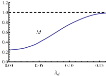
(a)   Magnetization

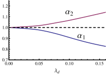
(b)   FS distortions

Figure 2: (color online) Magnetization $M$ and Fermi surface distortion parameters $\alpha_{1}$ and $\alpha_{2}$ vs the dimensionless dipolar coupling $\lambda_{d}$ for an s-wave coupling $\lambda_{s}=1.34$.

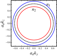
(a) $\lambda_{s}=1.34$, $\lambda_{d}=0.04$

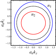
(b) $\lambda_{s}=1.34$, $\lambda_{d}=0.08$

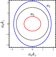
(c) $\lambda_{s}=1.37$, $\lambda_{d}=0.10$

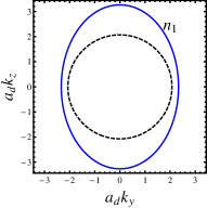
(d) $\lambda_{s}=1.37$, $\lambda_{d}=0.14$

Figure 3: (color online) a-d: Spin up and down FS, labeled by $n_{1}$ and $n_{2}$, for several values of $\lambda_{s}$ and $\lambda_{d}$ and fixed particle density $n$. $a_{d}=m\mu^{2}/\hbar^{2}$ is the dipole-dipole interaction length scale. Dashed lines: Free fermion FS.

The phase diagram shown in Fig. 1 exhibits a ferro-nematic phase and a paramagnetic phase, separated by a phase boundary consisting of a line of 1st order transitions that meets a line of continuous transitions at a tricritical point (labeled by $A$.) As expected the ferro-nematic state becomes more accessible as the $s$-wave coupling increases. This phase is fully polarized ($M=1$) for most of the phase diagram, except for a small region where the polarization is partial, $0<M<1$. In the ferro-nematic phase with partial polarization the up and down Fermi surfaces are unequally distorted, while in the fully polarized regime only one distorted up FS exists. Partial magnetization in the conventional Stoner transition occurs for $\lambda_{d}=0$ and $4/3<\lambda_{s}<2^{2/3}$, where the up and down FS become distorted even for arbitrarily small values of the dipolar coupling (see Fig. 2.) From the structure of the free energy for small values of $Q_{1}=\alpha_{1}-1$, $Q_{2}=\alpha_{2}-1$ and $M$ (valid in the vicinity of the continuous transition) we see that the dipolar interaction leads to a leading term of the form $M(Q_{1}-Q_{2})$, which is invariant under $1\leftrightarrow 2$. Since the ferromagnetic state is already favored by the contact term, this term also favors $Q_{1}<0$ and $Q_{2}>0$.

In the ferro-nematic phase the $SU(2)$ spin symmetry of the Hamiltonian is broken down to the residual $U(1)\cong SO(2)$ invariance of this uniaxial state. The equilibrium FS of the up and down spin components are shown in Fig. 3 for several values of of the coupling constants. Both FS’s are invariant under $SO(2)$ rigid rotations about $\mathbf{M}$.

The total energy, the equilibrium values of the FS distortions and the magnetization are functions of the particle density $n=N/V$. The pressure $P=-(\partial E/\partial V)_{N}$, chemical potential $\mu=(\partial E/\partial N)_{V}$ and the compressibility $K^{-1}=n(\partial P/\partial n)$ can be computed straightforwardly, and decrease monotonically as the dipolar coupling increases, see Fig. 4. The compressibility vanishes at $\lambda_{d}^{c}\simeq 0.52$ Sogo et al. (2009); com where the Fermi gas becomes (formally) unstable to collapseins .

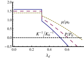
Figure 4: (color online) Pressure (broken), bulk compressibility (full) and chemical potential (dashed) (normalized to their values at the non-interacting Fermi gas) vs the dimensionless dipolar coupling $\lambda_{d}$, for $\lambda_{s}=0.8$. At $\lambda_{d}\sim 0.3$ there is a 1st order paramagnetic-ferro-nematic transition. The gas becomes unstable at $\lambda_{d}\simeq 0.52$.

In current experiments on cold atoms it is possible to prepare a two-component Fermi gas out of the hyperfine manifold of the atom. One can imagine, a two-component dipolar Fermi gas made out of, say, the hyperfine manifold of strongly magnetic atom such as Dy. For ¹⁶³Dy with a density of $10^{13}$cm^-3, we estimate $\lambda_{d}\simeq 0.01$ cav ; chr . The recent experimental observation of itinerant (Stoner) ferromagnetism in ultra-cold gases of ⁶Li atomsJo et al. (2009) opens the possibility to detect the ferro-nematic state in the laboratory possibly by tuning the $s$-wave scattering amplitude. Depending on the strength of the dipole moment and of the $s$-wave coupling, the FS for the two components may differ considerably from the spherical shape, and free expansion experiments may be able to provide signatures of this state. Ferromagnetism in cold dilute systems interacting only by s-wave contact pseudo-potential has been difficult to observe as the spin states of fermions are conserved separately on the time scales of the experimentsDuine and MacDonald (2005). However, a ferro-nematic state can be set up experimentally in systems with a population imbalance of hyperfine states, which may also exhibit other anisotropic and inhomogeneous phases. In actual experiments the trap potential is anisotropic and weakly inhomogeneous. We estimate that such effects do not affect our main results provided the trap potential aspect ratios depart from 1 by perhaps up to about 30%. Nevertheless, the anisotropy acts as a weak symmetry breaking field, that orients the ferro-nematic order.

In this work we have shown the existence a new phase of matter, the ferro-nematic Fermi fluid, a ground state of a dipolar Fermi gas with short range interactions with a spontaneous magnetization and long range orientational order. In this state, the up and down FS manifolds have unequal shapes and volumes. Since rotational invariance in real space and in spin space is simultaneously spontaneously broken in this state, it supports a rich spectrum of Goldstone excitations. As a result the fluid is an optically anisotropic medium whose properties that may be detected by light scattering experiments.

We thank B. L. Lev, B. Hsu, K. Sun, and B. Uchoa for many discussions. EF thanks the Kavli Institute for Theoretical Physics (KITP) of the University of California Santa Barbara for hospitality. This work was supported in part by the National Science Foundation under the grants DMR 0758462 (EF) at the University of Illinois, and PHY05-51164 (EF) at KITP, and by the Office of Science, U.S. Department of Energy under contracts DE-FG02-91ER45439 (EF, BMF) through the University of Illinois Frederick Seitz Materials Research Laboratory.

References

- Miyakawa et al. (2008) T. Miyakawa, T. Sogo, and H. Pu, Phys. Rev. A 77, 061603(R) (2008).
- Sogo et al. (2009) T. Sogo, L. He, T. Miyakawa, S. Yi, H. Lu, and H. Pu, New J. Phys. 11, 055017 (2009).
- Fregoso et al. (2009) B. M. Fregoso, K. Sun, E. Fradkin, and B. L. Lev, New J. Phys. 11, 103003 (2009).
- Kivelson et al. (1998) S. A. Kivelson, E. Fradkin, and V. J. Emery, Nature 393, 550 (1998).
- Oganesyan et al. (2001) V. Oganesyan, S. A. Kivelson, and E. Fradkin, Phys. Rev. B 64, 195109 (2001).
- Sun et al. (2008) K. Sun, B. M. Fregoso, M. J. Lawler, and E. Fradkin, Phys. Rev. B 78, 085124 (2008).
- Doniach and Sondheimer (1998) S. Doniach and E. H. Sondheimer, Green’s Functions For Solid State Physicists (Imperial College Press, 1998).
- (8) Ref.Mahanti and Jha (2007) used a similar variational state to argue that the dipolar Fermi gas is fully polarized.
- Mahanti and Jha (2007) S. D. Mahanti and S. S. Jha, Phys. Rev. E 76, 062101 (2007).
- Brochard and de Gennes (1970) F. Brochard and P. G. de Gennes, J. Physique (Paris) 31, 691 (1970).
- Seul and Andelman (1995) M. Seul and D. Andelman, Science 267, 477 (1995).
- Fomin et al. (1978) I. A. Fomin, C. J. Pethick, and J. W. Serene, Phys Rev. Lett. 40, 1144 (1978).
- Leefer et al. (2009) N. Leefer, A. Cingoz, and D. Budker, Optics Lett. 34, 2548 (2009).
- (14) A nematic-spin-nematic Kivelson et al. (2003); Wu et al. (2007) is a 2D state invariant under a rotation by followed by a spin flip. The uniaxial 3D ferro-nematic state does not have this property, as its up FS and down FS are not equivalent under a rotation.
- Kivelson et al. (2003) S. A. Kivelson, I. P. Bindloss, E. Fradkin, V. Oganesyan, J. M. Tranquada, A. Kapitulnik, and C. Howald, Rev. Mod. Phys. 75, 1201 (2003).
- Wu et al. (2007) C. Wu, K. Sun, E. Fradkin, and S. C. Zhang, Phys. Rev. B 75, 115103 (2007).
- Duine and MacDonald (2005) R. A. Duine and A. H. MacDonald, Phys Rev Lett 95, 230403 (2005).
- (18) Sogo et al Sogo et al. (2009) estimated that the homogeneous fully polarized dipolar Fermi gas becomes unstable at . The correct value is .
- (19) Short-range interactions tend to suppress this instability.
- (20) Dy has , and .Leefer et al. (2009) It is not described by this simple two-state model.
- (21) Dipolar atoms such as 52Cr have been cooled and a Bose-Einstein condensate has been observedBeaufulis et al. (2008). 53Cr is a fermion and, if cooled to low enough temperatures, could also be a candidate for a ferro-nematic state.
- Beaufulis et al. (2008) Q. Beaufils, R. Chicireanu, T. Zanon, B. Laburthe-Tolra, E. Maréchal, L. Vernac, J. C. Keller, and O. Gorceix, Phys Rev. A 77, 061601(R) (2008).
- Jo et al. (2009) G. B. Jo, Y. R. Lee, J. H. Choi, C. A. Christiansen, T. H. Kim, J. H. Thywissen, D. E. Pritchard, and W. Ketterle, Science 325, 1521 (2009).