Strong exciton-plasmon coupling in semiconducting carbon nanotubes

Abstract

We study theoretically the interactions of excitonic states with surface electromagnetic modes of small-diameter ($\,\lesssim\!1$ nm) semiconducting single-walled carbon nanotubes. We show that these interactions can result in strong exciton-surface-plasmon coupling. The exciton absorption line shape exhibits Rabi splitting $\sim 0.1$ eV as the exciton energy is tuned to the nearest interband surface plasmon resonance of the nanotube. We also show that the quantum confined Stark effect may be used as a tool to control the exciton binding energy and the nanotube band gap in carbon nanotubes in order, e. g., to bring the exciton total energy in resonance with the nearest interband plasmon mode. The exciton-plasmon Rabi splitting we predict here for an individual carbon nanotube is close in its magnitude to that previously reported for hybrid plasmonic nanostructures artificially fabricated of organic semiconductors on metallic films. We expect this effect to open up paths to new tunable optoelectronic device applications of semiconducting carbon nanotubes.

I Introduction

Single-walled carbon nanotubes (CNs) are quasi-one-dimensional (1D) cylindrical wires consisting of graphene sheets rolled-up into cylinders with diameters $\sim\!1-10$ nm and lengths $\sim\!1-10^{4}\,~{}\mu$m Dresselhaus ; Dai ; Zheng ; Huang . CNs are shown to be useful as miniaturized electronic, electromechanical, and chemical devices Baughman , scanning probe devices Popescu , and nanomaterials for macroscopic composites Trancik . The area of their potential applications was recently expanded to nanophotonics Bondarev06 ; Bondarev07 ; Bondarev07jem ; Bondarev07os after the demonstration of controllable single-atom incapsulation into CNs Shimoda ; Jeong ; Jeongtsf ; Khazaei , and even to quantum cryptography since the experimental evidence was reported for quantum correlations in the photoluminescence spectra of individual nanotubes Imamoglu .

For pristine (undoped) single-walled CNs, the numerical calculations predicting large exciton binding energies ($\sim\!0.3\!-\!0.6$ eV) in semiconducting CNs Pedersen03 ; Pedersen04 ; Capaz  and even in some small-diameter ($\sim\!0.5$ nm) metallic CNs Spataru04 , followed by the results of various exciton photoluminescence measurements Imamoglu ; Wang04 ; Wang05 ; Hagen05 ; Plentz05 ; Avouris08 , have become available. These works, together with other reports investigating the role of effects such as intrinsic defects Hagen05 ; Prezhdo08 , exciton-phonon interactions Plentz05 ; Prezhdo08 ; Perebeinos05 ; Lazzeri05 ; Piscanec , external magnetic and electric fields Zaric ; Perebeinos07 ; Srivastava , reveal the variety and complexity of the intrinsic optical properties of CNs Dresselhaus07 .

Here we develop a theory for the interactions between excitonic states and surface electromagnetic (EM) modes in small-diameter ($\lesssim\!1$ nm) semiconducting single-walled CNs. We demonstrate that such interactions can result in a strong exciton-surface-plasmon coupling due to the presence of low-energy ($\sim\!0.5\!-\!2$ eV) weakly-dispersive interband plasmon modes Pichler98 and large exciton excitation energies $\sim\!1$ eV Spataru05 ; Ma in small-diameter CNs. Previous studies have been focused on artificially fabricated hybrid plasmonic nanostructures, such as dye molecules in organic polymers deposited on metallic films Bellessa , semiconductor quantum dots coupled to metallic nanoparticles Govorov , or nanowires Fedutik , where one material carries the exciton and another one carries the plasmon. Our results are particularly interesting since they reveal the fundamental EM phenomenon — the strong exciton-plasmon coupling — in an individual quasi-1D nanostructure, a carbon nanotube.

The paper is organized as follows. Section II presents the general Hamiltonian of the exciton interaction with vacuum-type quantized surface EM modes of a single-walled CN. No external EM field is assumed to be applied. The vacuum–type–field we consider is created by CN surface EM fluctuations. In describing the exciton–field interaction on the CN surface, we use our recently developed Green function formalism to quantize the EM field in the presence of quasi-1D absorbing bodies Bondarev02 ; Bondarev04 ; Bondarev04pla ; Bondarev04ssc ; Bondarev05 ; Bondarev06trends . The formalism follows the original line of the macroscopic quantum electrodynamics (QED) approach developed by Welsch and coworkers to correctly describe medium-assisted electromagnetic vacuum effects in dispersing and absorbing media VogelWelsch ; ScheelWelsch ; BuhmannWelsch (also refs. therein). Section III explains how the interaction introduced in Sec. II results in the coupling of the excitonic states to the nanotube’s surface plasmon modes. Here we derive, calculate and discuss the characteristics of the coupled exciton–plasmon excitations, such as the dispersion relation, the plasmon density of states (DOS), and the optical absorption line shape, for particular semiconducting CNs of different diameters. We also analyze how the electrostatic field applied perpendicular to the CN axis affects the CN band gap, the exciton binding energy, and the surface plasmon energy, to explore the tunability of the exciton-surface-plasmon coupling in CNs. The summary and conclusions of the work are given in Sec. IV. All the technical details about the construction and diagonalization of the exciton–field Hamiltonian, the EM field Green tensor derivation, the perpendicular electrostatic field effect, are presented in the Appendices in order not to interrupt the flow of the arguments and results.

II Exciton-electromagnetic-field interaction on the nanotube surface

We consider the vacuum-type EM interaction of an exciton with the quantized surface electromagnetic fluctuations of a single-walled semiconducting CN by using our recently developed Green function formalism to quantize the EM field in the presence of quasi-1D absorbing bodies Bondarev02 ; Bondarev04 ; Bondarev04pla ; Bondarev04ssc ; Bondarev05 ; Bondarev06trends . No external EM field is assumed to be applied. The nanotube is modelled by an infinitely thin, infinitely long, anisotropically conducting cylinder with its surface conductivity obtained from the realistic band structure of a particular CN. Since the problem has the cylindrical symmetry, the orthonormal cylindrical basis $\{\mathbf{e}_{r},\mathbf{e}_{\varphi},\mathbf{e}_{z}\}$ is used with the vector $\mathbf{e}_{z}$ directed along the nanotube axis as shown in Fig. 1. Only the axial conductivity, $\sigma_{zz}$, is taken into account, whereas the azimuthal one, $\sigma_{\varphi\varphi}$, being strongly suppressed by the transverse depolarization effect Benedict ; Tasaki ; Li ; Marinop ; Ando ; Kozinsky , is neglected.

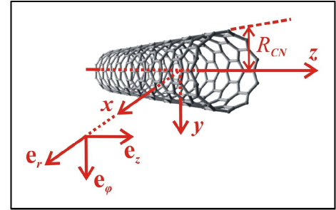
Figure 1: (Color online) The geometry of the problem.

The total Hamiltonian of the coupled exciton-photon system on the nanotube surface is of the form

$$\hat{H}=\hat{H}_{F}+\hat{H}_{ex}+\hat{H}_{int},$$ (1)

where the three terms represent the free (medium-assisted) EM field, the free (non-interacting) exciton, and their interaction, respectively. More explicitly, the second quantized field Hamiltonian is

$$\hat{H}_{F}\!=\!\sum_{\mathbf{n}}\int_{0}^{\infty}\!\!\!d\omega\,\hbar\omega\hat{f}^{\dagger}(\mathbf{n},\omega)\hat{f}(\mathbf{n},\omega),$$ (2)

where the scalar bosonic field operators $\hat{f}^{\dagger}(\mathbf{n},\omega)$ and $\hat{f}(\mathbf{n},\omega)$ create and annihilate, respectively, the surface EM excitation of frequency $\omega$ at an arbitrary point $\mathbf{n}\!=\!\mathbf{R}_{n}\!=\!\{R_{CN},\varphi_{n},z_{n}\}$ associated with a carbon atom (representing a lattice site – Fig. 1) on the surface of the CN of radius $R_{CN}$. The summation is made over all the carbon atoms, and in the following it is replaced by the integration over the entire nanotube surface according to the rule

$$\sum_{\mathbf{n}}\!\ldots=\frac{1}{S_{0}}\int\!d\mathbf{R}_{n}\!\ldots=\frac{1}{S_{0}}\int_{0}^{2\pi}\!\!\!\!d\varphi_{n}R_{CN}\!\int_{-\infty}^{\infty}\!\!\!\!dz_{n}\!\ldots,$$ (3)

where $S_{0}\!=\!(3\sqrt{3}/4)b^{2}$ is the area of an elementary equilateral triangle selected around each carbon atom in a way to cover the entire surface of the nanotube, $b\!=\!1.42$ Å is the carbon-carbon interatomic distance.

The second quantized Hamiltonian of the free exciton (see, e.g., Ref. Haken ) on the CN surface is of the form

$$\hat{H}_{ex}\!=\!\!\!\sum_{\mathbf{n},\mathbf{m},f}\!\!\!E_{f}(\mathbf{n})B^{\dagger}_{\mathbf{n}+\mathbf{m},f}B_{\mathbf{m},f}\!=\!\sum_{\mathbf{k},f}E_{f}(\mathbf{k})B^{\dagger}_{\mathbf{k},f}B_{\mathbf{k},f},$$ (4)

where the operators $B^{\dagger}_{\mathbf{n},f}$ and $B_{\mathbf{n},f}$ create and annihilate, respectively, an exciton with the energy $E_{f}(\mathbf{n})$ in the lattice site $\mathbf{n}$ of the CN surface. The index $f\,(\neq\!0)$ refers to the internal degrees of freedom of the exciton. Alternatively,

$$B^{\dagger}_{\mathbf{k},f}=\frac{1}{\sqrt{N}}\sum_{\mathbf{n}}\!B^{\dagger}_{\mathbf{n},f}e^{i\mathbf{k}\cdot\mathbf{n}}~{}~{}~{}\mbox{and}~{}~{}~{}B_{\mathbf{k},f}=(B^{\dagger}_{\mathbf{k},f})^{\dagger}$$ (5)

create and annihilate the $f$-internal-state exciton with the quasi-momentum $\mathbf{k}\!=\!\{k_{\varphi},k_{z}\}$, where the azimuthal component is quantized due to the transverse confinement effect and the longitudinal one is continuous, $N$ is the total number of the lattice sites (carbon atoms) on the CN surface. The exciton total energy is then written in the form

$$E_{f}(\mathbf{k})=E_{exc}^{(f)}(k_{\varphi})+\frac{\hbar^{2}k_{z}^{2}}{2M_{ex}(k_{\varphi})}$$ (6)

Here, the first term represents the excitation energy

$$E_{exc}^{(f)}(k_{\varphi})=E_{g}(k_{\varphi})+E_{b}^{(f)}(k_{\varphi})$$ (7)

of the $f$-internal-state exciton with the (negative) binding energy $E_{b}^{(f)}$, created via the interband transition with the band gap

$$E_{g}(k_{\varphi})=\varepsilon_{e}(k_{\varphi})+\varepsilon_{h}(k_{\varphi}),$$ (8)

where $\varepsilon_{e,h}$ are transversely quantized azimuthal electron-hole subbands (see the schematic in Fig. 2). The second term in Eq. (6) represents the kinetic energy of the translational longitudinal movement of the exciton with the effective mass $M_{ex}=m_{e}+m_{h}$, where $m_{e}$ and $m_{h}$ are the (subband-dependent) electron and hole effective masses, respectively. The two equivalent free-exciton Hamiltonian representations are related to one another via the obvious orthogonality relationships

$$\frac{1}{N}\sum_{\mathbf{n}}e^{-i(\mathbf{k}-\mathbf{k}^{\prime})\cdot\mathbf{n}}=\delta_{\mathbf{k}\mathbf{k}^{\prime}},\;\;\frac{1}{N}\sum_{\mathbf{k}}e^{-i(\mathbf{n}-\mathbf{m})\cdot\mathbf{\mathbf{k}}}=\delta_{\mathbf{n}\mathbf{m}}$$ (9)

with the $\mathbf{k}$-summation running over the first Brillouin zone of the nanotube. The bosonic field operators in $\hat{H}_{F}$ are transformed to the $\mathbf{k}$-representation in the same way.

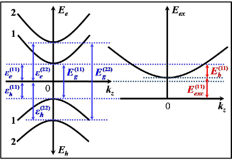
Figure 2: (Color online) Schematic of the two transversely quantized azimuthal electron-hole subbands (left), and the first-interband ground-internal-state exciton energy (right) in a small-diameter semiconducting carbon nanotube. Subbands with indices $j=1$ and 2 are shown, along with the optically allowed (exciton-related) interband transitions Ando . See text for notations.

The most general (non-relativistic, electric dipole) exciton-photon interaction on the nanotube surface can be written in the form (we use the Gaussian system of units and the Coulomb gauge; see details in Appendix A)

$$\hat{H}_{int}=\sum_{\mathbf{n},\mathbf{m},f}\int_{0}^{\infty}\!\!\!\!\!d\omega\,[\,\mbox{g}_{f}^{(+)}(\mathbf{n},\mathbf{m},\omega)B^{\dagger}_{\mathbf{n},f}\hskip 17.07182pt$$

$$-\;\mbox{g}_{f}^{(-)}(\mathbf{n},\mathbf{m},\omega)B_{\mathbf{n},f}\,]\,\hat{f}(\mathbf{m},\omega)+h.c.,$$ (10)

where

$$\mbox{g}_{f}^{(\pm)}(\mathbf{n},\mathbf{m},\omega)=\mbox{g}_{f}^{\perp}(\mathbf{n},\mathbf{m},\omega)\pm{\omega\over{\omega_{f}}}\,\mbox{g}_{f}^{\parallel}(\mathbf{n},\mathbf{m},\omega)$$ (11)

with

$$\mbox{g}_{f}^{\perp(\parallel)}(\mathbf{n},\mathbf{m},\omega)=-i\frac{4\omega_{f}}{c^{2}}\sqrt{\pi\hbar\omega\,\mbox{Re}\,\sigma_{zz}(R_{CN},\omega)}\hskip 14.22636pt$$

$$\times\;\;(\textbf{d}^{f}_{\mathbf{n}})_{z}\,^{\perp(\parallel)}G_{zz}(\mathbf{n},\mathbf{m},\omega)\hskip 39.83368pt$$ (12)

being the interaction matrix element where the exciton with the energy $E_{exc}^{(f)}=\hbar\omega_{f}$ is excited through the electric dipole transition $(\textbf{d}^{f}_{\mathbf{n}})_{z}\!=\!\langle 0|(\hat{\mathbf{d}}_{\mathbf{n}})_{z}|f\rangle$ in the lattice site n by the nanotube’s transversely (longitudinally) polarized surface EM modes. The modes are represented in the matrix element by the transverse (longitudinal) part of the Green tensor $zz$-component $G_{zz}(\mathbf{n},\mathbf{m},\omega)$ of the EM subsystem (Appendix B). This is the only Green tensor component we have to take into account. All the other components can be safely neglected as they are greatly suppressed by the strong transverse depolarization effect in CNs Benedict ; Tasaki ; Li ; Marinop ; Ando ; Kozinsky . As a consequence, only $\sigma_{zz}(R_{CN},\omega)$, the axial dynamic surface conductivity per unit length, is present in Eq.(12).

Equations (1)–(12) form the complete set of equations describing the exciton-photon coupled system on the CN surface in terms of the EM field Green tensor and the CN surface axial conductivity.

III Exciton-surface-plasmon coupling

For the following it is important to realize that the transversely polarized surface EM mode contribution to the interaction (10)–(12) is negligible compared to the longitudinally polarized surface EM mode contribution. As a matter of fact, ${}^{\perp}G_{zz}(\mathbf{n},\mathbf{m},\omega)\!\equiv\!0$ in the model of an infinitely thin cylinder we use here (Appendix B), thus yielding

$$\mbox{g}_{f}^{\perp}(\mathbf{n},\mathbf{m},\omega)\!\equiv\!0,~{}~{}~{}\mbox{g}_{f}^{(\pm)}(\mathbf{n},\mathbf{m},\omega)\!=\!\pm\frac{\omega}{\omega_{f}}\,\mbox{g}_{f}^{\parallel}(\mathbf{n},\mathbf{m},\omega)$$ (13)

in Eqs. (10)–(12). The point is that, because of the nanotube quasi-one-dimensionality, the exciton quasi-momentum vector and all the relevant vectorial matrix elements of the momentum and dipole moment operators are directed predominantly along the CN axis (the longitudinal exciton; see, however, Ref. UryuAndo ). This prevents the exciton from the electric dipole coupling to transversely polarized surface EM modes as they propagate predominantly along the CN axis with their electric vectors orthogonal to the propagation direction. The longitudinally polarized surface EM modes are generated by the electronic Coulomb potential (see, e.g., Ref. Landau ), and therefore represent the CN surface plasmon excitations. These have their electric vectors directed along the propagation direction. They do couple to the longitudinal excitons on the CN surface. Such modes were observed in Ref. Pichler98 . They occur in CNs both at high energies (well-known $\pi$-plasmon at $\sim\!6$ eV) and at comparatively low energies of $\sim\!0.5\!-\!2$ eV. The latter ones are related to the transversely quantized interband (inter-van Hove) electronic transitions. These weakly-dispersive modes Pichler98 ; Kempa02 are similar to the intersubband plasmons in quantum wells Kempa89 . They occur in the same energy range of $\sim\!1$ eV where the exciton excitation energies are located in small-diameter ($\lesssim\!1$ nm) semiconducting CNs Spataru05 ; Ma . In what follows we focus our consideration on the exciton interactions with these particular surface plasmon modes.

III.1 The dispersion relation

To obtain the dispersion relation of the coupled exciton-plasmon excitations, we transfer the total Hamiltonian (1)–(10) and (13) to the $\mathbf{k}$-representation using Eqs. (5) and (9), and then diagonalize it exactly by means of Bogoliubov’s canonical transformation technique (see, e.g., Ref. Davydov ). The details of the procedure are given in Appendix C. The Hamiltonian takes the form

$$\hat{H}=\!\!\!\sum_{\mathbf{k},\,\mu=1,2}\!\!\!\hbar\omega_{\mu}(\mathbf{k})\,\hat{\xi}^{\dagger}_{\mu}(\mathbf{k})\hat{\xi}_{\mu}(\mathbf{k})+E_{0}\,.$$ (14)

Here, the new operator

$$\hat{\xi}_{\mu}(\mathbf{k})=\sum_{f}\left[u_{\mu}^{\ast}(\mathbf{k},\omega_{f})B_{\mathbf{k},f}-v_{\mu}(\mathbf{k},\omega_{f})B_{-\mathbf{k},f}^{\dagger}\right]$$ (15)

$$+\int_{0}^{\infty}\!\!\!\!\!d\omega\left[u_{\mu}(\mathbf{k},\omega)\hat{f}(\mathbf{k},\omega)-v_{\mu}^{\ast}(\mathbf{k},\omega)\hat{f}^{\dagger}(-\mathbf{k},\omega)\right]$$

annihilates and $\hat{\xi}^{\dagger}_{\mu}(\mathbf{k})\!=\![\hat{\xi}_{\mu}(\mathbf{k})]^{\dagger}$ creates the exciton-plasmon excitation of branch $\mu$, the quantities $u_{\mu}$ and $v_{\mu}$ are appropriately chosen canonical transformation coefficients. The ”vacuum” energy $E_{0}$ represents the state with no exciton-plasmons excited in the system, and $\hbar\omega_{\mu}(\mathbf{k})$ is the exciton-plasmon energy given by the solution of the following (dimensionless) dispersion relation

$$x_{\mu}^{2}-\varepsilon_{f}^{2}-\varepsilon_{f}\frac{2}{\pi}\int_{0}^{\infty}\!\!\!\!\!dx\,\frac{x\,\bar{\Gamma}_{0}^{f}(x)\rho(x)}{x_{\mu}^{2}-x^{2}}=0\,.$$ (16)

Here,

$$x=\frac{\hbar\omega}{2\gamma_{0}},~{}~{}~{}x_{\mu}=\frac{\hbar\omega_{\mu}(\mathbf{k})}{2\gamma_{0}},~{}~{}~{}\varepsilon_{f}=\frac{E_{f}(\mathbf{k})}{2\gamma_{0}}$$ (17)

with $\gamma_{0}\!=\!2.7$ eV being the carbon nearest neighbor overlap integral entering the CN surface axial conductivity $\sigma_{zz}(R_{CN},\omega)$. The function

$$\bar{\Gamma}_{0}^{f}(x)=\frac{4|d^{f}_{z}|^{2}x^{3}}{3\hbar c^{3}}\left(\frac{2\gamma_{0}}{\hbar}\right)^{\!2}$$ (18)

with $d^{f}_{z}\!=\!\sum_{\mathbf{n}}\langle 0|(\hat{\mathbf{d}}_{\mathbf{n}})_{z}|f\rangle$ represents the (dimensionless) spontaneous decay rate, and

$$\rho(x)=\frac{3S_{0}}{16\pi\alpha R_{CN}^{2}}\;\mbox{Re}\frac{1}{\bar{\sigma}_{zz}(x)}$$ (19)

stands for the surface plasmon density of states (DOS) which is responsible for the exciton decay rate variation due to its coupling to the plasmon modes. Here, $\alpha\!=\!e^{2}/\hbar c\!=\!1/137$ is the fine-structure constant and $\bar{\sigma}_{zz}\!=\!2\pi\hbar\sigma_{zz}/e^{2}$ is the dimensionless CN surface axial conductivity per unit length.

Note that the conductivity factor in Eq. (19) equals

$$\mbox{Re}\frac{1}{\bar{\sigma}_{zz}(x)}=-\frac{4\alpha c}{R_{CN}}\left(\frac{\hbar}{2\gamma_{0}x}\right)\mbox{Im}\frac{1}{\epsilon_{zz}(x)-1}$$ (20)

in view of Eq. (17) and equation $\sigma_{zz}\!=\!-i\omega(\epsilon_{zz}\!-\!1)/4\pi S\rho_{T}$ representing the Drude relation for CNs, where $\epsilon_{zz}$ is the longitudinal (along the CN axis) dielectric function, $S$ and $\rho_{T}$ are the surface area of the tubule and the number of tubules per unit volume, respectively Bondarev04 ; Bondarev05 ; Tasaki . This relates very closely the surface plasmon DOS function (19) to the loss function $-\mbox{Im}(1/\epsilon)$ measured in Electron Energy Loss Spectroscopy (EELS) experiments to determine the properties of collective electronic excitations in solids Pichler98 .

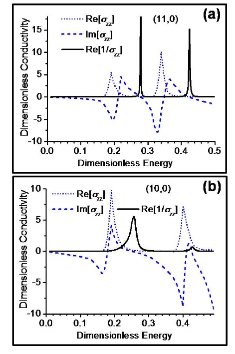
Figure 3: (Color online) (a),(b) Calculated dimensionless (see text) axial surface conductivities for the (11,0) and (10,0) CNs. The dimensionless energy is defined as [Energy]/$2\gamma_{0}$, according to Eq. (17).

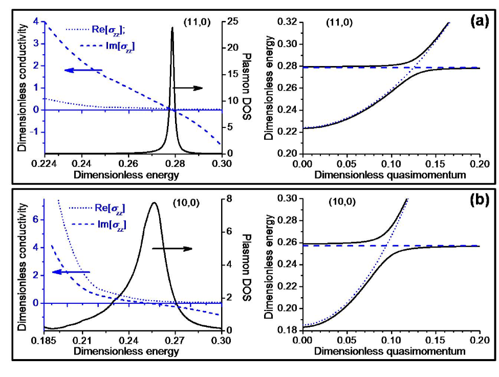
Figure 4: (Color online) (a),(b) Surface plasmon DOS and conductivities (left panels), and lowest bright exciton dispersion when coupled to plasmons (right panels) in (11,0) and (10,0) CNs, respectively. The dimensionless energy is defined as [Energy]/$2\gamma_{0}$, according to Eq. (17). See text for the dimensionless quasi-momentum.

Figure 3 shows the low-energy behaviors of the functions $\bar{\sigma}_{zz}(x)$ and $\mbox{Re}[1/\bar{\sigma}_{zz}(x)]$ for the (11,0) and (10,0) CNs ($R_{CN}=0.43$ nm and $0.39$ nm, respectively) we study here. We obtained them numerically as follows. First, we adapt the nearest-neighbor non-orthogonal tight-binding approach Valentin to determine the realistic band structure of each CN. Then, the room-temperature longitudinal dielectric functions $\epsilon_{zz}$ are calculated within the random-phase approximation LinShung97 ; EhrenreichCohen59 , which are then converted into the conductivities $\bar{\sigma}_{zz}$ by means of the Drude relation. Electronic dissipation processes are included in our calculations within the relaxation-time approximation (electron scattering length of $130R_{CN}$ was used Lazzeri05 ). We did not include excitonic many-electron correlations, however, as they mostly affect the real conductivity $\mbox{Re}(\bar{\sigma}_{zz})$ which is responsible for the CN optical absorption Pedersen04 ; Spataru04 ; Ando , whereas we are interested here in $\mbox{Re}(1/\bar{\sigma}_{zz})$ representing the surface plasmon DOS according to Eq. (19). This function is only non-zero when the two conditions, $\mbox{Im}[\bar{\sigma}_{zz}(x)]=0$ and $\mbox{Re}[\bar{\sigma}_{zz}(x)]\rightarrow 0$, are fulfilled simultaneously Kempa02 ; Kempa89 ; LinShung97 . These result in the peak structure of the function $\mbox{Re}(1/\bar{\sigma}_{zz})$ as is seen in Fig. 3. It is also seen from the comparison of Fig. 3 (b) with Fig. 3 (a) that the peaks broaden as the CN diameter decreases. This is consistent with the stronger hybridization effects in smaller-diameter CNs Blase94 .

Left panels in Figs. 4(a) and 4(b) show the lowest-energy plasmon DOS resonances calculated for the (11,0) and (10,0) CNs as given by the function $\rho(x)$ in Eq. (19). Also shown there are the corresponding fragments of the functions $\mbox{Re}[\bar{\sigma}_{zz}(x)]$ and $\mbox{Im}[\bar{\sigma}_{zz}(x)]$. In all graphs the lower dimensionless energy limits are set up to be equal to the lowest bright exciton excitation energy [$E^{(11)}_{exc}=1.21$ eV ($x=0.224$) and $1.00$ eV ($x=0.185$) for the (11,0) and (10,0) CN, respectively, as reported in Ref.Spataru05 by directly solving the Bethe-Salpeter equation]. Peaks in $\rho(x)$ are seen to coincide in energy with zeros of $\mbox{Im}[\bar{\sigma}_{zz}(x)]$ {or zeros of $\mbox{Re}[\epsilon_{zz}(x)]$}, clearly indicating the plasmonic nature of the CN surface excitations under consideration Kempa02 ; Kempa . They describe the surface plasmon modes associated with the transversely quantized interband electronic transitions in CNs Kempa02 . As is seen in Fig. 4 (and in Fig. 3), the interband plasmon excitations occur in CNs slightly above the first bright exciton excitation energy Ando , in the frequency domain where the imaginary conductivity (or the real dielectric function) changes its sign. This is a unique feature of the complex dielectric response function, the consequence of the general Kramers-Krönig relation VogelWelsch .

We further take advantage of the sharp peak structure of $\rho(x)$ and solve the dispersion equation (16) for $x_{\mu}$ analytically using the Lorentzian approximation

$$\rho(x)\!\approx\!\frac{\rho(x_{p})\Delta x_{p}^{2}}{(x-x_{p})^{2}+\Delta x_{p}^{2}}\,.$$ (21)

Here, $x_{p}$ and $\Delta x_{p}$ are, respectively, the position and the half-width-at-half-maximum of the plasmon resonance closest to the lowest bright exciton excitation energy in the same nanotube (as shown in the left panels of Fig. 4). The integral in Eq. (16) then simplifies to the form

$$\frac{2}{\pi}\int_{0}^{\infty}\!\!\!\!\!dx\,\frac{x\,\bar{\Gamma}_{0}^{f}(x)\rho(x)}{x_{\mu}^{2}-x^{2}}\approx\frac{F(x_{p})\Delta x_{p}^{2}}{x_{\mu}^{2}-x_{p}^{2}}\!\int_{0}^{\infty}\!\!\!\!\!\frac{dx}{(x-x_{p})^{2}+\Delta x_{p}^{2}}$$

$$=\frac{F(x_{p})\Delta x_{p}}{x_{\mu}^{2}-x_{p}^{2}}\left[\arctan\!\left(\frac{x_{p}}{\Delta x_{p}}\right)+\frac{\pi}{2}\right]$$

with $F(x_{p})=2x_{p}\bar{\Gamma}_{0}^{f}(x_{p})\rho(x_{p})/\pi$. This expression is valid for all $x_{\mu}$ apart from those located in the narrow interval $(x_{p}-\Delta x_{p},x_{p}+\Delta x_{p})$ in the vicinity of the plasmon resonance, provided that the resonance is sharp enough. Then, the dispersion equation becomes the biquadratic equation for $x_{\mu}$ with the following two positive solutions (the dispersion curves) of interest to us

$$x_{1,2}=\sqrt{\frac{\varepsilon_{f}^{2}+x_{p}^{2}}{2}\pm\frac{1}{2}\sqrt{(\varepsilon_{f}^{2}\!-x_{p}^{2})^{2}+F_{\!p}\,\varepsilon_{f}}}\,.$$ (22)

Here, $F_{\!p}=4F(x_{p})\Delta x_{p}(\pi-\Delta x_{p}/x_{p})$ with the $\arctan$-function expanded to linear terms in $\Delta x_{p}/x_{p}\ll 1$.

The dispersion curves (22) are shown in the right panels in Figs. 4(a) and 4(b) as functions of the dimensionless longitudinal quasi-momentum. In these calculations, we estimated the interband transition matrix element in $\bar{\Gamma}_{0}^{f}(x_{p})$ [Eq. (18)] from the equation $|d_{f}|^{2}=3\hbar\lambda^{3}/4\tau_{ex}^{rad}$ according to Hanamura’s general theory of the exciton radiative decay in spatially confined systems Hanamura , where $\tau_{ex}^{rad}$ is the exciton intrinsic radiative lifetime, and $\lambda=2\pi c\hbar/E$ with $E$ being the exciton total energy given in our case by Eq. (6). For zigzag-type CNs considered here, the first Brillouin zone of the longitudinal quasi-momentum is given by $-2\pi\hbar/3b\leq\hbar k_{z}\leq 2\pi\hbar/3b$ Dresselhaus ; Dai . The total energy of the ground-internal-state exciton can then be written as $E=E_{exc}+(2\pi\hbar/3b)^{2}t^{2}/2M_{ex}$ with $-1\leq t\leq 1$ representing the dimensionless longitudinal quasi-momentum. In our calculations we used the lowest bright exciton parameters $E^{(11)}_{exc}=1.21$ eV and $1.00$ eV, $\tau_{ex}^{rad}=14.3$ ps and $19.1$ ps, $M_{ex}=0.44m_{0}$ and $0.19m_{0}$ ($m_{0}$ is the free-electron mass) for the (11,0) CN and (10,0) CN, respectively, as reported in Ref.Spataru05 by directly solving the Bethe-Salpeter equation.

Both graphs in the right panels in Fig. 4 are seen to demonstrate a clear anticrossing behavior with the (Rabi) energy splitting $\sim\!0.1$ eV. This indicates the formation of the strongly coupled surface plasmon-exciton excitations in the nanotubes under consideration. It is important to realize that here we deal with the strong exciton-plasmon interaction supported by an individual quasi-1D nanostructure — a single-walled (small-diameter) semiconducting carbon nanotube, as opposed to the artificially fabricated metal-semiconductor nanostructures studied previuosly Bellessa ; Govorov ; Fedutik where the metallic component normally carries the plasmon and the semiconducting one carries the exciton. It is also important that the effect comes not only from the height but also from the width of the plasmon resonance as it is seen from the definition of the $F_{p}$ factor in Eq. (22). In other words, as long as the plasmon resonance is sharp enough (which is always the case for interband plasmons), so that the Lorentzian approximation (21) applies, the effect is determined by the area under the plasmon peak in the DOS function (19) rather than by the peak height as one would expect.

However, the formation of the strongly coupled exciton-plasmon states is only possible if the exciton total energy is in resonance with the energy of a surface plasmon mode. The exciton energy can be tuned to the nearest plasmon resonance in ways used for excitons in semiconductor quantum microcavities — thermally Reithmaier ; Yoshie ; Peter (by elevating sample temperature), or/and electrostatically MillerPRL ; Miller ; Zrenner ; Krenner (via the quantum confined Stark effect with an external electrostatic field applied perpendicular to the CN axis). As is seen from Eqs. (6) and (7), the two possibilities influence the different degrees of freedom of the quasi-1D exciton — the (longitudinal) kinetic energy and the excitation energy, respectively. Below we study the (less trivial) electrostatic field effect on the exciton excitation energy in carbon nanotubes.

III.2 The perpendicular electrostatic field effect

The optical properties of semiconducting CNs in an external electrostatic field directed along the nanotube axis were studied theoretically in Ref. Perebeinos07 . Strong oscillations in the band-to-band absorption and the quadratic Stark shift of the exciton absorption peaks with the field increase, as well as the strong field dependence of the exciton ionization rate, were predicted for CNs of different diameters and chiralities. Here, we focus on the perpendicular electrostatic field orientation. We study how the electrostatic field applied perpendicular to the CN axis affects the CN band gap, the exciton binding/excitation energy, and the interband surface plasmon energy, to explore the tunability of the strong exciton-plasmon coupling effect predicted above. The problem is similar to the well-known quantum confined Stark effect first observed for the excitons in semiconductor quantum wells MillerPRL ; Miller . However, the cylindrical surface symmetry of the excitonic states brings new peculiarities to the quantum confined Stark effect in CNs. In what follows we will generally be interested only in the lowest internal energy (ground) excitonic state, and so the internal state index $f$ in Eqs. (6) and (7) will be omitted for brevity.

Because the nanotube is modelled by a continuous, infinitely thin, anisotropically conducting cylinder in our macroscopic QED approach, the actual local symmetry of the excitonic wave function resulted from the graphene Brillouin zone structure is disregarded in our model (see, e.g., reviews Dresselhaus07 ; Ando ). The local symmetry is implicitly present in the surface axial conductivity though, which we calculate beforehand as described above EndNote1 .

We start with the Schrödinger equation for the electron located at $\textbf{r}_{e}=\{R_{CN},\varphi_{e},z_{e}\}$ and the hole located at $\textbf{r}_{h}=\{R_{CN},\varphi_{h},z_{h}\}$ on the nanotube surface. They interact with each other through the Coulomb potential $V(\textbf{r}_{e},\textbf{r}_{h})=-e^{2}/\epsilon|\textbf{r}_{e}\!-\textbf{r}_{h}|$, where $\epsilon=\epsilon_{zz}(0)$. The external electrostatic field $\textbf{F}=\{F,0,0\}$ is directed perpendicular to the CN axis (along the $x$-axis in Fig. 1). The Schrödinger equation is of the form

$$\left[\hat{H}_{e}(\textbf{F})+\hat{H}_{h}(\textbf{F})+V(\textbf{r}_{e},\textbf{r}_{h})\right]\!\Psi(\textbf{r}_{e},\textbf{r}_{h})=E\Psi(\textbf{r}_{e},\textbf{r}_{h})$$ (23)

with

$$\hat{H}_{e,h}(\textbf{F})=-\frac{\hbar^{2}}{2m_{e,h}}\left(\!\frac{1}{R_{CN}^{2}}\frac{\partial^{2}}{\partial\varphi^{2}_{e,h}}+\frac{\partial^{2}}{\partial z^{2}_{e,h}}\right)\!\mp e\textbf{r}_{e,h}\!\cdot\textbf{F}$$ (24)

We further separate out the translational and relative degrees of freedom of the electron-hole pair by transforming the longitudinal (along the CN axis) motion of the pair into its center-of-mass coordinates given by $Z=(m_{e}z_{e}+m_{h}z_{h})/M_{ex}$ and $z=z_{e}-z_{h}$. The exciton wave function is approximated as follows

$$\Psi(\textbf{r}_{e},\textbf{r}_{h})=e^{ik_{z}Z}\phi_{ex}(z)\psi_{e}(\varphi_{e})\psi_{h}(\varphi_{h}).$$ (25)

The complex exponential describes the exciton center-of-mass motion with the longitudinal quasi-momentum $k_{z}$ along the CN axis. The function $\phi_{ex}(z)$ represents the longitudinal relative motion of the electron and the hole inside the exciton. The functions $\psi_{e}(\varphi_{e})$ and $\psi_{h}(\varphi_{h})$ are the electron and hole subband wave functions, respectively, which represent their confined motion along the circumference of the cylindrical nanotube surface.

Each of the functions is assumed to be normalized to unity. Equations (23) and (24) are then rewritten in view of Eqs. (6)–(8) to yield

$$\left[-\frac{\hbar^{2}}{2m_{e}R_{CN}^{2}}\frac{\partial^{2}}{\partial\varphi^{2}_{e}}-eR_{CN}F\cos(\varphi_{e})\right]\!\psi_{e}(\varphi_{e})=\varepsilon_{e}\psi_{e}(\varphi_{e}),$$ (26)

$$\left[-\frac{\hbar^{2}}{2m_{h}R_{CN}^{2}}\frac{\partial^{2}}{\partial\varphi^{2}_{h}}+eR_{CN}F\cos(\varphi_{h})\right]\!\psi_{h}(\varphi_{h})\!=\!\varepsilon_{h}\psi_{h}(\varphi_{h})\!,$$ (27)

$$\left[-\frac{\hbar^{2}}{2\mu}\frac{\partial^{2}}{\partial\,\!z^{2}}+V_{\mbox{\small{eff}}}(z)\right]\!\phi_{ex}(z)=E_{b}\phi_{ex}(z),$$ (28)

where $\mu=m_{e}m_{h}/M_{ex}$ is the exciton reduced mass, and $V_{\mbox{\small eff}}$ is the effective longitudinal electron-hole Coulomb interaction potential given by

$$V_{\mbox{\small eff}}(z)=\!-\frac{e^{2}}{\epsilon}\!\int_{0}^{2\pi}\!\!\!\!\!\!d\varphi_{e}\!\!\int_{0}^{2\pi}\!\!\!\!\!\!d\varphi_{h}|\psi_{e}(\varphi_{e})|^{2}|\psi_{h}(\varphi_{h})|^{2}V(\varphi_{e},\varphi_{h},z)$$ (29)

with $V$ being the original electron-hole Coulomb potential written in the cylindrical coordinates as

$$V(\varphi_{e},\varphi_{h},z)=\!\frac{1}{\{z^{2}+4R_{CN}^{2}\sin^{2}[(\varphi_{e}\!-\varphi_{h})/2]\}^{1/2}}.$$ (30)

The exciton problem is now reduced to the 1D equation (28), where the exciton binding energy does depend on the perpendicular electrostatic field through the electron and hole subband functions $\psi_{e,h}$ given by the solutions of Eqs. (26) and (27) and entering the effective electron-hole Coulomb interaction potential (29).

The set of Eqs. (26)-(30) is analyzed in Appendix D. One of the main results obtained in there is that the effective Coulomb potential (29) can be approximated by an attractive cusp-type cutoff potential of the form

$$V_{\mbox{\small eff}}(z)\approx-\frac{e^{2}}{\epsilon[|z|+z_{0}(j,F)]},$$ (31)

where the cutoff parameter $z_{0}$ depends on the perpendicular electrostatic field strength and on the electron-hole azimuthal transverse quantization index $j=1,2,...$ (excitons are created in interband transitions involving valence and conduction subbands with the same quantization index Ando as shown in Fig. 2). Specifically,

$$z_{0}(j,F)\approx 2R_{CN}\frac{\pi-2\ln 2\,[1-\Delta_{j}(F)]}{\pi+2\ln 2\,[1-\Delta_{j}(F)]}$$ (32)

with $\Delta_{j}(F)$ given to the second order approximation in the electric field by

$$\Delta_{j}(F) \!\!\approx\!\! 2\mu M_{ex}\frac{e^{2}R_{CN}^{6}w^{2}_{j}}{\hbar^{4}}\,F^{2},$$ (33)

$$w_{j} \!\!=\!\! \frac{\theta(j\!-\!2)}{1-2j}+\frac{1}{1+2j},$$

where $\theta(x)$ is the unit step function. Approximation (31) is formally valid when $z_{0}(j,F)$ is much less than the exciton Bohr radius $a_{B}^{\ast}$ $(=\epsilon\hbar^{2}/\mu e^{2})$ which is estimated to be $\sim\!10R_{CN}$ for the first ($j\!=\!1$ in our notations here) exciton in CNs Pedersen03 . As is seen from Eqs. (32) and (33), this is always the case for the first exciton for those fields where the perturbation theory applies, i. e. when $\Delta_{1}(F)<1$ in Eq. (33).

Equation (28) with the potential (31) formally coincides with the one studied by Ogawa and Takagahara in their treatments of excitonic effects in 1D semiconductors with no external electrostatic field applied Takagahara . The only difference in our case is that our cutoff parameter (32) is field dependent. We therefore follow Ref. Takagahara and find the ground-state binding energy $E^{(11)}_{b}$ for the first exciton we are interested in here from the transcendental equation

$$\ln\!\left[\frac{2z_{0}(1,F)}{\hbar}\sqrt{2\mu|E^{(11)}_{b}|}\,\right]+\frac{1}{2}\sqrt{\frac{|E^{(11)}_{b}|}{Ry^{\ast}}}=0.$$ (34)

In doing so, we first find the exciton Rydberg energy, $Ry^{\ast}$ $(=\!\mu e^{4}/2\hbar^{2}\epsilon^{2})$, from this equation at $F\!=\!0$. We use the diameter- and chirality-dependent electron and hole effective masses from Ref. Jorio , and the first bright exciton binding energy of 0.76 eV for both (11,0) and (10,0) CN as reported in Ref. Capaz from ab initio calculations. We obtain $Ry^{\ast}=4.02$ eV and $0.57$ eV for the (11,0) tube and (10,0) tube, respectively. The difference of about one order of magnitude reflects the fact that these are the semiconducting CNs of different types — type-I and type-II, respectively, based on $(2n+m)$ families Jorio . The parameters $Ry^{\ast}$ thus obtained are then used to find $|E^{(11)}_{b}|$ as functions of $F$ by numerically solving Eq. (34) with $z_{0}(1,F)$ given by Eqs. (32) and (33).

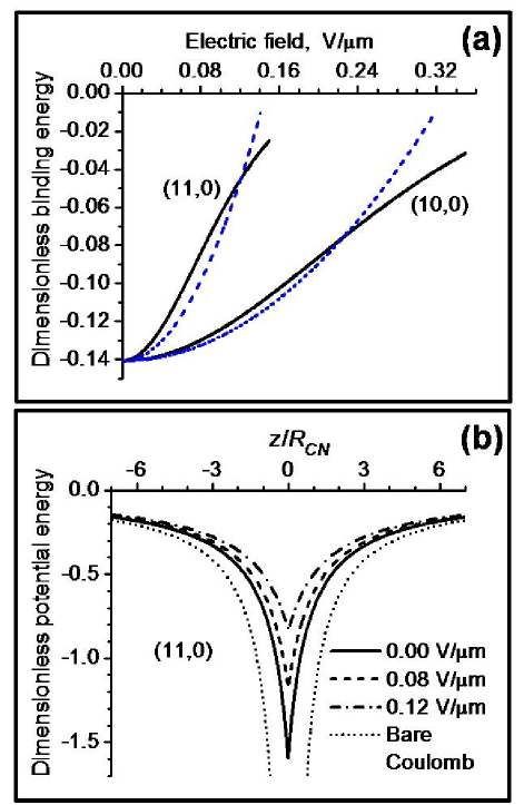
Figure 5: (Color online) (a) Calculated binding energies of the first bright exciton in the (11,0) and (10,0) CNs as functions of the perpendicular electrostatic field applied. Solid lines are the numerical solutions to Eq. (34), dashed lines are the quadratic approximations as given by Eq. (35). (b) Field dependence of the effective cutoff Coulomb potential (31) in the (11,0) CN. The dimensionless energy is defined as [Energy]/$2\gamma_{0}$, according to Eq. (17).

The calculated (negative) binding energies are shown by the solid lines in Fig. 5(a). Also shown there by dashed lines are the functions

$$E^{(11)}_{b}(F)\approx E^{(11)}_{b}[1-\Delta_{1}(F)]$$ (35)

with $\Delta_{1}(F)$ given by Eq. (33). They are seen to be fairly good analytical (quadratic in field) approximations to the numerical solutions of Eq. (34) in the range of not too large fields. The exciton binding energy decreases very rapidly in its absolute value as the field increases. Fields of only $\sim\!0.1-0.2$ V/$\mu$m are required to decrease $|E^{(11)}_{b}|$ by a factor of $\sim\!2$ for the CNs considered here. The reason is the perpendicular field shifts up the ”bottom” of the effective potential (31) as shown in Fig. 5(b) for the (11,0) CN. This makes the potential shallower and pushes bound excitonic levels up, thereby decreasing the exciton binding energy in its absolute value. As this takes place, the shape of the potential does not change, and the longitudinal relative electron-hole motion remains finite at all times. As a consequence, no tunnel exciton ionization occurs in the perpendicular field, as opposed to the longitudinal electrostatic field (Franz-Keldysh) effect studied in Ref. Perebeinos07 where the non-zero field creates the potential barrier separating out the regions of finite and infinite relative motion and the exciton becomes ionized as the electron tunnels to infinity.

The binding energy is only the part of the exciton excitation energy (7). Another part comes from the band gap energy (8), where $\varepsilon_{e}$ and $\varepsilon_{h}$ are given by the solutions of Eqs. (26) and (27), respectively. Solving them to the leading (second) order perturbation theory approximation in the field (Appendix D), one obtains

$$E^{(jj)}_{g}(F)\approx E^{(jj)}_{g}\!\left[1-\frac{m_{e}\Delta_{j}(F)}{2M_{ex}j^{2}w_{j}}-\frac{m_{h}\Delta_{j}(F)}{2M_{ex}j^{2}w_{j}}\right]\!,$$ (36)

where the electron and hole subband shifts are written separately. This, in view of Eq. (33), yields the first band gap field dependence in the form

$$E^{(11)}_{g}(F)\approx E^{(11)}_{g}\!\left[1-\frac{3}{2}\,\Delta_{1}(F)\right]\!,$$ (37)

The bang gap decrease with the field in Eq. (37) is stronger than the opposite effect in the negative exciton binding energy given (to the same order approximation in field) by Eq. (35). Thus, the first exciton excitation energy (7) will be gradually decreasing as the perpendicular field increases, shifting the exciton absorption peak to the red. This is the basic feature of the quantum confined Stark effect observed previously in semiconductor nanomaterials MillerPRL ; Miller ; Zrenner ; Krenner . The field dependences of the higher interband transitions exciton excitation energies are suppressed by the rapidly (quadratically) increasing azimuthal quantization numbers in the denominators of Eqs. (33) and (36).

Lastly, the perpendicular field dependence of the interband plasmon resonances can be obtained from the frequency dependence of the axial surface conductivity due to excitons (see Ref. Ando and refs. therein). One has

$$\sigma^{ex}_{zz}(\omega)\sim\!\!\!\sum_{j=1,2,...}\!\frac{-i\hbar\omega f_{j}}{[E^{(jj)}_{exc}]^{2}\!-(\hbar\omega)^{2}\!-2i\hbar^{2}\omega/\tau},$$ (38)

where $f_{j}$ and $\tau$ are the exciton oscillator strength and relaxation time, respectively. The plasmon frequencies are those at which the function $\mbox{Re}[1/\sigma^{ex}_{zz}(\omega)]$ has maxima. Testing it for maximum in the domain $E^{(11)}_{exc}\!\!<\!\hbar\omega<\!E^{(22)}_{exc}$, one finds the first interband plasmon resonance energy to be (in the limit $\tau\!\rightarrow\!\infty$)

$$E^{(11)}_{p}=\sqrt{\frac{[E^{(11)}_{exc}]^{2}+[E^{(22)}_{exc}]^{2}}{2}}\,.$$ (39)

Using the field dependent $E^{(11)}_{exc}$ given by Eqs. (7), (35) and (37), and neglecting the field dependence of $E^{(22)}_{exc}$, one obtains to the second order approximation in the field

$$E^{(11)}_{p}(F)\approx E^{(11)}_{p}\!\left[1-\frac{1+\!E^{(11)}_{g}\!/2E^{(11)}_{exc}}{1+\!E^{(22)}_{exc}\!/E^{(11)}_{exc}}\;\Delta_{1}(F)\right]\!.$$ (40)

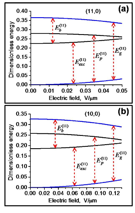
Figure 6: (Color online) (a),(b) Calculated dependences of the first bright exciton parameters in the (11,0) and (10,0) CNs, respectively, on the electrostatic field applied perpendicular to the nanotube axis. The dimensionless energy is defined as [Energy]/$2\gamma_{0}$, according to Eq. (17). The energy is measured from the top of the first unperturbed hole subband.

Figure 6 shows the results of our calculations of the field dependences for the first bright exciton parameters in the (11,0) and (10,0) CNs. The energy is measured from the top of the first unperturbed hole subband (as shown in Fig. 2, right panel). The binding energy field dependence was calculated numerically from Eq. (34) as described above [shown in Fig. 5 (a)]. The band gap field dependence and the plasmon energy field dependence were calculated from Eqs. (36) and (40), respectively. The zero-field excitation energies and zero-field binding energies were taken to be those reported in Ref. Spataru05 and in Ref. Capaz , respectively, and we used the diameter- and chirality-dependent electron and hole effective masses from Ref. Jorio . As is seen in Fig. 6 (a) and (b), the exciton excitation energy and the interband plasmon energy experience red shift in both nanotubes as the field increases. However, the excitation energy red shift is very small (barely seen in the figures) due to the negative field dependent contribution from the exciton binding energy. So, $E^{(11)}_{exc}(F)$ and $E^{(11)}_{p}(F)$ approach each other as the field increases, thereby bringing the total exciton energy (6) in resonance with the surface plasmon mode due to the non-zero longitudinal kinetic energy term at finite temperature EndNote2 . Thus, the electrostatic field applied perpendicular to the CN axis (the quantum confined Stark effect) may be used to tune the exciton energy to the nearest interband plasmon resonance, to put the exciton-surface plasmon interaction in small-diameter semiconducting CNs to the strong-coupling regime.

III.3 The optical absorption

Here we analyze the longitudinal exciton absorption line shape as its energy is tuned to the nearest interband surface plasmon resonance. Only longitudinal excitons (excited by light polarized along the CN axis) couple to the surface plasmon modes as discussed at the very beginning of this section (see Ref. UryuAndo for the perpendicular light exciton absorption in CNs). We follow the optical absorption/emission lineshape theory developed recently for atomically doped CNs Bondarev06 . (Obviously, the absorption line shape coincides with the emission line shape if the monochromatic incident light beam is used in the absorption experiment.) When the $f$-internal state exciton is excited and the nanotube’s surface EM field subsystem is in vacuum state, the time-dependent wave function of the whole system ”exciton+field” is of the form EndNote1

$$|\psi(t)\rangle = \sum_{{\bf k},f}C_{f}(\textbf{k},t)\,e^{-i\tilde{E}_{f}({\bf k})t/\hbar}|\{1_{f}(\textbf{k})\}\rangle_{ex}|\{0\}\rangle$$

$$+ \sum_{\bf k}\int_{0}^{\infty}\!\!\!\!\!\!d\omega\,C(\textbf{k},\omega,t)\,e^{-i\omega t}|\{0\}\rangle_{ex}|\{1(\mathbf{k},\omega)\}\rangle.$$

Here, $|\{1_{f}(\textbf{k})\}\rangle_{ex}$ is the excited single-quantum Fock state with one exciton and $|\{1(\textbf{k},\omega)\}\rangle$ is that with one surface photon. The vacuum states are $|\{0\}\rangle_{ex}$ and $|\{0\}\rangle$ for the exciton subsystem and field subsystem, respectively. The coefficients $C_{f}(\textbf{k},t)$ and $C(\textbf{k},\omega,t)$ stand for the population probability amplitudes of the respective states of the whole system. The exciton energy is of the form $\tilde{E}_{f}(\textbf{k})\!=\!E_{f}(\textbf{k})\!-i\hbar/\tau$ with $E_{f}(\textbf{k})$ given by Eq. (6) and $\tau$ being the phenomenological exciton relaxation time constant [assumed to be such that $\hbar/\tau\!\ll\!E_{f}(\textbf{k})$] to account for other possible exciton relaxation processes. From the literature we have $\tau_{ph}\sim 30\!-\!100$ fs for the exciton-phonon scattering Perebeinos07 , $\tau_{d}\sim 50$ ps for the exciton scattering by defects Hagen05 ; Prezhdo08 , and $\tau_{rad}\sim 10\,\mbox{ps}-10\,\mbox{ns}$ for the radiative decay of excitons Spataru05 . Thus, the scattering by phonons is the most likely exciton relaxation mechanism.

We transform the total Hamiltonian (1)–(10) to the $\mathbf{k}$-representation using Eqs. (5) and (9) (see Appendix A), and apply it to the wave function in Eq. (III.3). We obtain the following set of the two simultaneous differential equations for the coefficients $C_{f}(\textbf{k},t)$ and $C(\textbf{k},\omega,t)$ from the time dependent Schrödinger equation

$$\mbox{\it\.{C}}_{f}(\textbf{k},t)\,e^{-i\tilde{E}_{f}({\bf\!\,k})t/\hbar}\!\! = \!\!-\frac{i}{\hbar}\sum_{{\bf\!\,k^{\prime}}}\int_{0}^{\infty}\!\!\!\!\!d\omega\,\mbox{g}^{(+)}_{f}(\mathbf{k},\mathbf{k}^{\prime}\!,\omega)\hskip 28.45274pt$$

$$\times \!C(\textbf{k}^{\prime}\!,\omega,t)\,e^{-i\omega\!\,t},$$

$$\mbox{\it\.{C}\,}(\textbf{k}^{\prime}\!,\omega,t)\,e^{-i\omega\!\,t}\delta_{{\bf\!\,k}{\bf\!\,k}^{\prime}}\!\! = \!\!-\frac{i}{\hbar}\sum_{f}\,[\mbox{g}^{(+)}_{f}(\mathbf{k},\mathbf{k}^{\prime}\!,\omega)]^{\ast}\hskip 28.45274pt$$

$$\times \!C_{f}(\textbf{k},t)\,e^{-i\tilde{E}_{f}({\bf\!\,k})t/\hbar}.$$

The $\delta$-symbol on the left in Eq. (III.3) ensures that the momentum conservation is fulfilled in the exciton-photon transitions, so that the annihilating exciton creates the surface photon with the same momentum and vice versa. In terms of the probability amplitudes above, the exciton emission intensity distribution is given by the final state probability at very long times corresponding to the complete decay of all initially excited excitons,

$$I(\omega)\! = \!|C(\mathbf{k},\omega,t\!\rightarrow\!\infty)|^{2}=\frac{1}{\hbar^{2}}\sum_{f}|\mbox{g}^{(+)}_{f}(\mathbf{k},\mathbf{k},\omega)|^{2}$$ (44)

$$\times \!\left|\int_{0}^{\infty}\!\!\!\!\!dt^{\prime}\,C_{f}(\textbf{k},t^{\prime})\,e^{-i[\tilde{E}_{f}({\bf\!\,k})-\hbar\omega]t^{\prime}\!/\hbar}\right|^{2}\!.$$

Here, the second equation is obtained by the formal integration of Eq. (III.3) over time under the initial condition $C\,(\textbf{k},\omega,0)\!=\!0$. The emission intensity distribution is thus related to the exciton population probability amplitude $C_{f}(\mathbf{k},t)$ to be found from Eq. (III.3).

The set of simultaneous equations (III.3) and (III.3) [and Eq. (44), respectively] contains no approximations except the (commonly used) neglect of many-particle excitations in the wave function (III.3). We now apply these equations to the exciton-surface-plasmon system in small-diameter semiconducting CNs. The interaction matrix element in Eqs. (III.3) and (III.3) is then given by the $\mathbf{k}$-transform of Eq. (13), and has the following property (Appendix C)

$$\frac{1}{2\gamma_{0}\hbar}\,|\mbox{g}^{(+)}_{f}(\mathbf{k},\mathbf{k},\omega)|^{2}=\frac{1}{2\pi}\,\bar{\Gamma}_{0}^{f}(x)\rho(x)$$ (45)

with $\bar{\Gamma}_{0}^{f}(x)$ and $\rho(x)$ given by Eqs. (18) and (19), respectively. We further substitute the result of the formal integration of Eq. (III.3) [with $C\,(\textbf{k},\omega,0)\!=\!0$] into Eq. (III.3), use Eq. (45) with $\rho(x)$ approximated by the Lorentzian (21), calculate the integral over frequency analytically, and differentiate the result over time to obtain the following second order ordinary differential equation for the exciton probability amplitude [dimensionless variables, Eq. (17)]

$$\mbox{\it\"{C}}_{f}(\beta)+[\Delta x_{p}-\Delta\varepsilon_{f}+i(x_{p}-\varepsilon_{f})]\mbox{\it\.{C}}_{f}(\beta)+(X_{f}/2)^{2}C_{f}(\beta)\!=\!0,$$

where $X_{f}\!=\![2\Delta x_{p}\bar{\Gamma}_{f}(x_{p})]^{1/2}$ with $\bar{\Gamma}_{f}(x_{p})\!=\!\bar{\Gamma}_{0}^{f}(x_{p})\rho(x_{p})$, $\Delta\varepsilon_{f}=\hbar/2\gamma_{0}\tau$, $\beta=2\gamma_{0}t/\hbar$ is the dimensionless time, and the k-dependence is omitted for brevity. When the total exciton energy is close to a plasmon resonance, $\varepsilon_{f}\!\approx\!x_{p}$, the solution of this equation is easily found to be

$$C_{f}(\beta)\!\!\! \approx \!\!\!\frac{1}{2}\left(\!1+\frac{\delta x}{\sqrt{\delta x^{2}-X_{f}^{2}}}\right)e^{-\left(\delta x-\sqrt{\delta x^{2}-X_{f}^{2}}\right)\beta/2}\hskip 14.22636pt$$

$$+ \!\!\!\frac{1}{2}\left(\!1-\frac{\delta x}{\sqrt{\delta x^{2}-X_{f}^{2}}}\right)e^{-\left(\delta x+\sqrt{\delta x^{2}-X_{f}^{2}}\right)\beta/2},$$

where $\delta x=\Delta x_{p}-\Delta\varepsilon_{f}>0$ and $X_{f}\!=\![2\Delta x_{p}\bar{\Gamma}_{f}(\varepsilon_{f})]^{1/2}$. This solution is valid when $\varepsilon_{f}\!\approx\!x_{p}$ regardless of the strength of the exciton-surface-plasmon coupling. It yields the exponential decay of the excitons into plasmons, $|C_{f}(\beta)|^{2}\!\approx\!\exp[-\bar{\Gamma}_{f}(\varepsilon_{f})\beta]$, in the weak coupling regime where the coupling parameter $(X_{f}/\delta x)^{2}\!\ll\!1$. If, on the other hand, $(X_{f}/\delta x)^{2}\!\gg\!1$, then the strong coupling regime occurs, and the decay of the excitons into plasmons proceeds via damped Rabi oscillations, $|C_{f}(\beta)|^{2}\!\approx\!\exp(-\delta x\beta)\cos^{2}(X_{f}\beta/2)$. This is very similar to what was earlier reported for an excited two-level atom near the nanotube surface Bondarev02 ; Bondarev04 ; Bondarev04pla ; Bondarev06trends . Note, however, that here we have the exciton-phonon scattering as well, which facilitates the strong exciton-plasmon coupling by decreasing $\delta x$ in the coupling parameter. In other words, the phonon scattering broadens the (longitudinal) exciton momentum distribution Bondarev05Ps , thus effectively increasing the fraction of the excitons with $\varepsilon_{f}\!\approx\!x_{p}$.

In view of Eqs. (45) and (III.3), the exciton emission intensity (44) in the vicinity of the plasmon resonance takes the following (dimensionless) form

$$\bar{I}(x)\approx\bar{I}_{0}(\varepsilon_{f})\sum_{f}\left|\int_{0}^{\infty}\!\!\!\!\!\!d\beta\,C_{f}(\beta)\,e^{i(x-\varepsilon_{f}+i\Delta\varepsilon_{f})\beta}\right|^{2},$$ (47)

where $\bar{I}(x)\!=\!2\gamma_{0}I(\omega)/\hbar$ and $\bar{I}_{0}\!=\!\bar{\Gamma}_{f}(\varepsilon_{f})/2\pi$. After some algebra, this results in

$$\bar{I}(x)\approx\frac{\bar{I}_{0}(\varepsilon_{f})\,[(x-\varepsilon_{f})^{2}+\Delta x_{p}^{2}]}{[(x-\varepsilon_{f})^{2}-X_{f}^{2}/4]^{2}+(x-\varepsilon_{f})^{2}(\Delta x_{p}^{2}+\Delta\varepsilon_{f}^{2})}\,,$$ (48)

where $\Delta x_{p}^{2}>\Delta\varepsilon_{f}^{2}$. The summation sign over the exciton internal states is omitted since only one internal state contributes to the emission intensity in the vicinity of the sharp plasmon resonance.

The line shape in Eq. (48) is mainly determined by the coupling parameter $(X_{f}/\Delta x_{p})^{2}$. It is clearly seen to be of a symmetric two-peak structure in the strong coupling regime where $(X_{f}/\Delta x_{p})^{2}\gg 1$. Testing it for extremum, we obtain the peak frequencies to be

$$x_{1,2}=\varepsilon_{f}\pm\frac{X_{f}}{2}\sqrt{\sqrt{1+8\left(\!\frac{\Delta x_{p}}{X_{f}}\right)^{2}}\!\!-4\left(\!\frac{\Delta x_{p}}{X_{f}}\right)^{2}}$$

[terms $\sim\!(\Delta x_{p})^{2}(\Delta\varepsilon_{f})^{2}/X_{f}^{4}$ are neglected], with the Rabi splitting $x_{1}-x_{2}\!\approx\!X_{f}$. In the weak coupling regime where $(X_{f}/\Delta x_{p})^{2}\ll 1$, the frequencies $x_{1}$ and $x_{2}$ become complex, indicating that there are no longer peaks at these frequencies. As this takes place, Eq. (48) is approximated with the weak coupling condition, the fact that $x\!\sim\!\varepsilon_{f}$, and $X_{f}^{2}=2\Delta x_{p}\bar{\Gamma}_{f}(\varepsilon_{f})$, to yield the Lorentzian

$$\tilde{I}(x)\approx\frac{\bar{I}_{0}(\varepsilon_{f})/[1+(\Delta\varepsilon_{f}/\Delta x_{p})^{2}]}{(x-\varepsilon_{f})^{2}+\left[\bar{\Gamma}_{f}(\varepsilon_{f})/2\sqrt{1+(\Delta\varepsilon_{f}^{\!}/\Delta x_{p})^{2}}\;\right]^{2}}$$

peaked at $x=\varepsilon_{f}$, whose half-width-at-half-maximum is slightly narrower, however, than $\bar{\Gamma}_{f}(\varepsilon_{f})/2$ it should be if the exciton-plasmon relaxation were the only relaxation mechanism in the system. The reason is the competing phonon scattering takes excitons out of resonance with plasmons, thus decreasing the exciton-plasmon relaxation rate. We therefore conclude that the phonon scattering does not affect the exciton emission/absorption line shape when the exciton-plasmon coupling is strong (it facilitates the strong coupling regime to occur, however, as was noticed above), and it narrows the (Lorentzian) emission/absorption line when the exciton-plasmon coupling is weak.

Calculated exciton emission/absorption lineshapes, as given by Eq. (48) for the CNs under consideration, are shown in Fig. 7 (a) and (b). The exciton energies are assumed to be tuned, e. g. by means of the quantum confined Stark effect discussed in Sec. III.B, to the nearest plasmon resonances (shown by the vertical dashed lines in the figure). We used $\tau_{ph}\!=\!30$ fs as reported in Ref. Perebeinos05 . The line (Rabi) splitting effect is seen to be $\sim 0.1$ eV, indicating the strong exciton-plasmon coupling with the formation of the mixed surface plasmon-exciton excitations. The splitting is larger in the smaller diameter nanotubes, and is not masked by the exciton-phonon scattering.

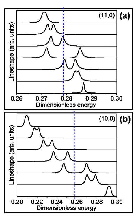
Figure 7: (Color online) (a),(b) Exciton absorption/emission lineshapes as the exciton energies are tuned to the nearest plasmon resonance energies (vertical dashed lines in here; see Fig. 3 and left panels in Fig. 4) in the (11,0) and (10,0) nanotubes, respectively. The dimensionless energy is defined as [Energy]/$2\gamma_{0}$, according to Eq. (17).

IV Conclusions

We have shown that the strong exciton-surface-plasmon coupling effect with characteristic exciton absorption line (Rabi) splitting $\sim\!0.1$ eV exists in small-diameter ($\lesssim\!1$ nm) semiconducting CNs. The splitting is almost as large as the typical exciton binding energies in such CNs ($\sim\!0.3-0.8$ eV Pedersen03 ; Pedersen04 ; Wang05 ; Capaz ), and of the same order of magnitude as the exciton-plasmon Rabi splitting in organic semiconductors ($\sim\!180$ meV Bellessa ). It is much larger than the exciton-polariton Rabi splitting in semiconductor microcavities ($\sim\!140-400\,\mu\mbox{eV}\,$Reithmaier ; Yoshie ; Peter ), or the exciton-plasmon Rabi splitting in hybrid semiconductor-metal nanoparticle molecules Govorov .

Since the formation of the strongly coupled mixed exciton-plasmon excitations is only possible if the exciton total energy is in resonance with the energy of an interband surface plasmon mode, we have analyzed possible ways to tune the exciton energy to the nearest surface plasmon resonance. Specifically, the exciton energy may be tuned to the nearest plasmon resonance in ways used for the excitons in semiconductor quantum microcavities — thermally (by elevating sample temperature) Reithmaier ; Yoshie ; Peter , and/or electrostatically MillerPRL ; Miller ; Zrenner ; Krenner (via the quantum confined Stark effect with an external electrostatic field applied perpendicular to the CN axis). The two possibilities influence the different degrees of freedom of the quasi-1D exciton — the (longitudinal) kinetic energy and the excitation energy, respectively.

We have studied how the perpendicular electrostatic field affects the exciton excitation energy and interband plasmon resonance energy (the quantum confined Stark effect). Both of them are shown to shift to the red due to the decrease in the CN band gap as the field increases. However, the exciton red shift is much less than the plasmon one because of the decrease in the absolute value of the negative binding energy, which contributes largely to the exciton excitation energy. The exciton excitation energy and interband plasmon energy approach as the field increases, thereby bringing the total exciton energy in resonance with the plasmon mode due to the non-zero longitudinal kinetic energy term at finite temperature.

Lastly, the noteworthy message we would like to deliver in this paper is that the strong exciton-surface-plasmon coupling we predict here occurs in an individual CN as opposed to various artificially fabricated hybrid plasmonic nanostructures mentioned above. We strongly believe this phenomenon, along with its tunability feature via the quantum confined Stark effect we have demonstrated, opens up new paths for the development of CN based tunable optoelectronic device applications in areas such as nanophotonics, nanoplasmonics, and cavity QED. One straightforward application like this is the CN photoluminescence control by means of the exciton-plasmon coupling tuned electrostatically via the quantum confined Stark effect. This complements the microcavity controlled CN infrared emitter application reported recentlyAvouris08 , offering the advantage of less stringent fabrication requirements at the same time since the planar photonic microcavity is no longer required. Electrostatically controlled coupling of two spatially separated (weakly localized) excitons to the same nanotube’s plasmon resonance would result in their entanglement Bondarev07 ; Bondarev07jem ; Bondarev07os , the phenomenon that paves the way for CN based solid-state quantum information applications. Moreover, CNs combine advantages such as electrical conductivity, chemical stability, and high surface area that make them excellent potential candidates for a variety of more practical applications, including efficient solar energy conversion Trancik , energy storage Shimoda , and optical nanobiosensorics AngChem09 . However, the photoluminescence quantum yield of individual CNs is relatively low, and this hinders their uses in the aforementioned applications. CN bundles and films are proposed to be used to surpass the poor performance of individual tubes. The theory of the exciton-plasmon coupling we have developed here, being extended to include the inter-tube interaction, complements currently available ’weak-coupling’ theories of the exciton-plasmon interactions in low-dimensional nanostructures Govorov ; GovorovPRB with the very important case of the strong coupling regime. Such an extended theory (subject of our future publication) will lay the foundation for understanding inter-tube energy transfer mechanisms that affect the efficiency of optoelectronic devices made of CN bundles and films, as well as it will shed more light on the recent photoluminescence experiments with CN bundles Munich ; Ferrari and multi-walled CNs Hirori , revealing their potentialities for the development of high-yield, high-performance optoelectronics applications with CNs.

Appendix A  Exciton interaction with the surface electromagnetic field

We follow our recently developed QED formalism to describe vacuum-type EM effects in the presence of quasi-1D absorbing and dispersive bodies Bondarev02 ; Bondarev04 ; Bondarev04pla ; Bondarev04ssc ; Bondarev05 ; Bondarev06trends . The treatment begins with the most general EM interaction of the surface charge fluctuations with the quantized surface EM field of a single-walled CN. No external field is assumed to be applied. The CN is modelled by a neutral, infinitely long, infinitely thin, anisotropically conducting cylinder. Only the axial conductivity of the CN, $\sigma_{zz}$, is taken into account, whereas the azimuthal one, $\sigma_{\varphi\varphi}$, is neglected being strongly suppressed by the transverse depolarization effect Benedict ; Tasaki ; Li ; Marinop ; Ando ; Kozinsky . Since the problem has the cylindrical symmetry, the orthonormal cylindrical basis $\{\mathbf{e}_{r},\mathbf{e}_{\varphi},\mathbf{e}_{z}\}$ is used with the vector $\mathbf{e}_{z}$ directed along the nanotube axis as shown in Fig. 1. The interaction has the following form (Gaussian system of units)

$$\hat{H}_{int}=\hat{H}_{int}^{(1)}+\hat{H}_{int}^{(2)}\hskip 65.44142pt$$ (49)

$$=-\sum_{\mathbf{n},i}\frac{q_{i}}{m_{i}c}\hat{\mathbf{A}}(\mathbf{n}+\hat{\mathbf{r}}_{\mathbf{n}}^{(i)})\!\cdot\!\left[\hat{\mathbf{p}}_{\mathbf{n}}^{(i)}-\frac{q_{i}}{2c}\hat{\mathbf{A}}(\mathbf{n}+\hat{\mathbf{r}}_{\mathbf{n}}^{(i)})\right]$$

$$+\sum_{\mathbf{n},i}q_{i}\hat{\varphi}(\mathbf{n}+\hat{\mathbf{r}}_{\mathbf{n}}^{(i)}),\hskip 65.44142pt$$

where $c$ is the speed of light, $m_{i}$, $q_{i}$, $\hat{\mathbf{r}}_{\mathbf{n}}^{(i)}$, and $\hat{\mathbf{p}}_{\mathbf{n}}^{(i)}$ are, respectively, the masses, charges, coordinate operators and momenta operators of the particles (electrons and nucleus) residing at the lattice site $\mathbf{n}\!=\!\mathbf{R}_{n}\!=\!\{R_{CN},\varphi_{n},z_{n}\}$ associated with a carbon atom (see Fig. 1) on the surface of the CN of radius $R_{CN}$. The summation is taken over the lattice sites, and may be substituted with the integration over the CN surface using Eq. (3). The vector potential operator $\hat{\mathbf{A}}$ and the scalar potential operator $\hat{\varphi}$ represent the nanotube’s transversely polarized and longitudinally polarized surface EM modes, respectively. They are written in the Schrödinger picture as follows

$$\hat{\mathbf{A}}(\mathbf{n})=\int_{0}^{\infty}\!\!\!\!\!d\omega\frac{c}{i\omega}\,\hat{\underline{\mathbf{E}}}^{\perp}(\mathbf{n},\omega)+h.c.,$$ (50)

$$-\bm{\nabla}_{\!\mathbf{n}}\,\hat{\varphi}(\mathbf{n})=\int_{0}^{\infty}\!\!\!\!\!d\omega\,\hat{\underline{\mathbf{E}}}^{\parallel}(\mathbf{n},\omega)+h.c..$$ (51)

We use the Coulomb gauge whereby $\bm{\nabla}_{\!\mathbf{n}}\!\cdot\!\hat{\mathbf{A}}(\mathbf{n})\!=\!0$, or equivalently, $[\hat{\mathbf{p}}_{\mathbf{n}}^{(i)}\!,\hat{\mathbf{A}}(\mathbf{n}+\hat{\mathbf{r}}_{\mathbf{n}}^{(i)})]=0$.

The total electric field operator of the CN-modified EM field is given for an arbitrary $\mathbf{r}$ in the Schrödinger picture by

$$\hat{\mathbf{E}}(\mathbf{r})=\!\int_{0}^{\infty}\!\!\!\!\!d\omega\,\hat{\underline{\mathbf{E}}}(\mathbf{r},\omega)+h.c.\hskip 19.91684pt$$ (52)

$$=\!\int_{0}^{\infty}\!\!\!\!\!d\omega\,[\hat{\underline{\mathbf{E}}}^{\perp}(\mathbf{r},\omega)+\hat{\underline{\mathbf{E}}}^{\parallel}(\mathbf{r},\omega)]+h.c.$$

with the transversely (longitudinally) polarized Fourier-domain field components defined as

$$\underline{\hat{\mathbf{E}}}^{\perp(\parallel)}(\mathbf{r},\omega)=\!\int\!d\mathbf{r}^{\prime}\,\bm{\delta}^{\perp(\parallel)}(\mathbf{r}-\mathbf{r}^{\prime})\cdot\underline{\hat{\mathbf{E}}}(\mathbf{r}^{\prime}\!,\omega),$$ (53)

where

$$\delta^{\parallel}_{\alpha\beta}(\mathbf{r})=-\nabla_{\alpha}\nabla_{\beta}{1\over{4\pi r}}\,,\hskip 5.69046pt$$ (54)

$$\delta^{\perp}_{\alpha\beta}(\mathbf{r})=\delta_{\alpha\beta}\,\delta(\mathbf{r})-\delta^{\parallel}_{\alpha\beta}(\mathbf{r})$$

are the longitudinal and transverse dyadic $\delta$-functions, respectively. The total field operator (52) satisfies the set of the Fourier-domain Maxwell equations

$$\bm{\nabla}\times\underline{\hat{\mathbf{E}}}(\mathbf{r},\omega)=ik\,\underline{\hat{\mathbf{H}}}(\mathbf{r},\omega),\hskip 34.14322pt$$ (55)

$$\bm{\nabla}\times\underline{\hat{\mathbf{H}}}(\mathbf{r},\omega)=-ik\,\underline{\hat{\mathbf{E}}}(\mathbf{r},\omega)+{4\pi\over{c}}\,\underline{\hat{\mathbf{I}}}(\mathbf{r},\omega),$$ (56)

where $\underline{\hat{\mathbf{H}}}=(ik)^{-1}\bm{\nabla}\times\underline{\hat{\mathbf{E}}}$ is the magnetic field operator, $k=\omega/c$, and

$$\underline{\hat{\mathbf{I}}}(\mathbf{r},\omega)=\sum_{\mathbf{n}}\delta(\mathbf{r}-\mathbf{n})\,\underline{\hat{\mathbf{J}}\!}\,(\mathbf{n},\omega),$$ (57)

is the exterior current operator with the current density defined as follows

$$\underline{\hat{\mathbf{J}}\!}\,(\mathbf{n},\omega)\!=\!\sqrt{\hbar\omega\,\mbox{Re}\sigma_{zz}(R_{CN},\omega)\over{\pi}}\,\hat{f}(\mathbf{n},\omega)\textbf{e}_{z}$$ (58)

to ensure preservation of the fundamental QED equal-time commutation relations (see, e.g., VogelWelsch ) for the EM field components in the presence of a CN. Here, $\sigma_{zz}$ is the CN surface axial conductivity per unit length, and $\hat{f}(\mathbf{n},\omega)$ along with its counter-part $\hat{f}^{\dagger}(\mathbf{n},\omega)$ are the scalar bosonic field operators which annihilate and create, respectively, single-quantum EM field excitations of frequency $\omega$ at the lattice site $\mathbf{n}$ of the CN surface. They satisfy the standard bosonic commutation relations

$$[\hat{f}(\mathbf{n},\omega),\hat{f}^{\dagger}(\mathbf{m},\omega^{\prime})]=\delta_{\mathbf{n}\mathbf{m}}\,\delta(\omega-\omega^{\prime}),\hskip 19.91684pt$$ (59)

$$[\hat{f}(\mathbf{n},\omega),\hat{f}(\mathbf{m},\omega^{\prime})]=[\hat{f}^{\dagger}(\mathbf{n},\omega),\hat{f}^{\dagger}(\mathbf{m},\omega^{\prime})]=0.$$

One further obtains from Eqs. (55)–(58) that

$$\underline{\hat{\mathbf{E}}}(\mathbf{r},\omega)=ik{4\pi\over{c}}\sum_{\mathbf{n}}\mathbf{G}(\mathbf{r},\mathbf{n},\omega)\!\cdot\!\underline{\hat{\mathbf{J}}\!}\,(\mathbf{n},\omega),$$ (60)

and, according to Eqs. (52) and (53),

$$\underline{\hat{\mathbf{E}}}^{\perp(\parallel)}(\mathbf{r},\omega)=ik{4\pi\over{c}}\sum_{\mathbf{n}}\,\!^{\perp(\parallel)}\mathbf{G}(\mathbf{r},\mathbf{n},\omega)\!\cdot\!\underline{\hat{\mathbf{J}}\!}\,(\mathbf{n},\omega),$$ (61)

where ${}^{\perp}\mathbf{G}$ and ${}^{\parallel}\mathbf{G}$ are the transverse part and the longitudinal part, respectively, of the total Green tensor $\mathbf{G}=\,\!^{\perp}\mathbf{G}+\,\!^{\parallel}\mathbf{G}$ of the classical EM field in the presence of the CN. This tensor satisfies the equation

$$\sum_{\alpha=r,\varphi,z}\!\!\!\left(\bm{\nabla}\!\times\bm{\nabla}\!\times-\,k^{2}\right)_{\!z\alpha}G_{\alpha z}(\mathbf{r},\mathbf{n},\omega)=\delta(\mathbf{r}-\mathbf{n})$$ (62)

together with the radiation conditions at infinity and the boundary conditions on the CN surface.

All the ’discrete’ quantities in Eqs. (57)–(62) may be equivalently rewritten in continuous variables in view of Eq. (3). Being applied to the identity $1=\sum_{\mathbf{m}}\delta_{\mathbf{n}\mathbf{m}}$, Eq. (3) yields

$$\delta_{\mathbf{n}\mathbf{m}}=S_{0}\,\delta(\mathbf{R}_{n}\!-\mathbf{R}_{m}).$$ (63)

This requires to redefine

$$\hat{f}(\mathbf{n},\omega)=\sqrt{S_{0}}\,\hat{f}(\mathbf{R}_{n},\omega),~{}\hat{f}^{\dagger}(\mathbf{n},\omega)=\sqrt{S_{0}}\,\hat{f}^{\dagger}(\mathbf{R}_{n},\omega)$$ (64)

in the commutation relations (59). Similarly, from Eq. (60), in view of Eqs. (3), (58) and (64), one obtains

$$\mathbf{G}(\mathbf{r},\mathbf{n},\omega)=\sqrt{S_{0}}\,\mathbf{G}(\mathbf{r},\mathbf{R}_{n},\omega),$$ (65)

which is also valid for the transverse and longitudinal Green tensors in Eq. (61).

Next, we make the series expansions of the interactions $\hat{H}_{int}^{(1)}$ and $\hat{H}_{int}^{(2)}$ in Eq. (49) about the lattice site $\mathbf{n}$ to the first non-vanishing terms,

$$\hat{H}_{int}^{(1)}\approx-\sum_{\mathbf{n},i}\frac{q_{i}}{m_{i}c}\hat{\mathbf{A}}(\mathbf{n})\cdot\hat{\mathbf{p}}_{\mathbf{n}}^{(i)}+\sum_{\mathbf{n},i}\frac{q_{i}^{2}}{2m_{i}c^{2}}\hat{\mathbf{A}}^{2}(\mathbf{n}),\hskip 14.22636pt$$ (66)

$$\hat{H}_{int}^{(2)}\approx\sum_{\mathbf{n},i}q_{i}\mathbf{\nabla}_{\!\mathbf{n}}\,\hat{\varphi}(\mathbf{n})\cdot\hat{\mathbf{r}}_{\mathbf{n}}^{(i)},\hskip 56.9055pt$$ (67)

and introduce the single-lattice-site Hamiltonian

$$\hat{H}_{\mathbf{n}}=\varepsilon_{0}|0\rangle\langle 0|+\sum_{f}(\varepsilon_{0}+\hbar\omega_{f})|f\rangle\langle\,\!f|$$ (68)

with the completeness relation

$$|0\rangle\langle 0|+\sum_{f}|f\rangle\langle\,\!f|=\hat{I}.$$ (69)

Here, $\varepsilon_{0}$ is the energy of the ground state $|0\rangle$ (no exciton excited) of the carbon atom associated with the lattice site $\mathbf{n}$, $\varepsilon_{0}+\hbar\omega_{f}$ is the energy of the excited carbon atom in the quantum state $|f\rangle$ with one $f$-internal-state exciton formed of the energy $E_{exc}^{(f)}=\hbar\omega_{f}$. In view of Eqs. (68) and (69), one has

$$\hat{\mathbf{p}}_{\mathbf{n}}^{(i)}=m_{i}\frac{d\,\hat{\mathbf{r}}_{\mathbf{n}}^{(i)}}{dt}=\frac{m_{i}}{i\hbar}\,[\hat{\mathbf{r}}_{\mathbf{n}}^{(i)},\hat{H}_{\mathbf{n}}]=\frac{m_{i}}{i\hbar}\,\hat{I}\,[\hat{\mathbf{r}}_{\mathbf{n}}^{(i)},\hat{H}_{\mathbf{n}}]\,\hat{I}\hskip 14.22636pt$$

$$\approx\frac{m_{i}}{i\hbar}\sum_{f}\hbar\omega_{f}\!\left(\langle 0|\hat{\mathbf{r}}_{\mathbf{n}}^{(i)}|f\rangle\,\!B_{\mathbf{n},f}\!-\langle\,\!f|\hat{\mathbf{r}}_{\mathbf{n}}^{(i)}|0\rangle\,\!B^{\dagger}_{\mathbf{n},f}\right)\hskip 19.91684pt$$ (70)

and

$$\hat{\mathbf{r}}_{\mathbf{n}}^{(i)}=\hat{I}\,\hat{\mathbf{r}}_{\mathbf{n}}^{(i)}\hat{I}\approx\sum_{f}\!\left(\langle 0|\hat{\mathbf{r}}_{\mathbf{n}}^{(i)}|f\rangle\,\!B_{\mathbf{n},f}+\langle\,\!f|\hat{\mathbf{r}}_{\mathbf{n}}^{(i)}|0\rangle\,\!B^{\dagger}_{\mathbf{n},f}\right)\!,$$ (71)

where $\langle 0|\hat{\mathbf{r}}_{\mathbf{n}}^{(i)}|f\rangle=\langle\,\!f|\hat{\mathbf{r}}_{\mathbf{n}}^{(i)}|0\rangle$ in view of the hermitian and real character of the coordinate operator. The operators $B_{\mathbf{n},f}\!=\!|0\rangle\langle f|$ and $B^{\dagger}_{\mathbf{n},f}\!=\!|f\rangle\langle 0|$ create and annihilate, respectively, the $f$-internal-state exciton at the lattice site $\mathbf{n}$, and exciton-to-exciton transitions are neglected. In addition, we also have

$$\delta_{ij}\delta_{\alpha\beta}={i\over{\hbar}}\,[(\hat{\mathbf{p}}_{\mathbf{n}}^{(i)})_{\alpha},(\hat{\mathbf{r}}_{\mathbf{n}}^{(j)})_{\beta}],$$ (72)

where $\alpha,\beta=r,\varphi,z$. Substituting these into Eqs. (66) and (67) [commutator (72) goes into the second term of Eq. (66) which is to be pre-transformed as follows $\sum_{i,j,\alpha,\beta}q_{i}q_{j}\hat{A}(\mathbf{n})_{\alpha}\hat{A}(\mathbf{n})_{\beta}\delta_{ij}\delta_{\alpha\beta}/2m_{i}c^{2}$], one arrives at the following (electric dipole) approximation of Eq. (49)

$$\hat{H}_{int}=\hat{H}_{int}^{(1)}+\hat{H}_{int}^{(2)}\hskip 71.13188pt$$ (73)

$$=-\sum_{\mathbf{n},f}\frac{i\omega_{f}}{c}\,\textbf{d}^{f}_{\mathbf{n}}\cdot\hat{\textbf{A}}(\textbf{n})\!\left[B^{\dagger}_{\mathbf{n},f}\!-B_{\mathbf{n},f}+\frac{i}{\hbar\,\!c}\,\textbf{d}^{f}_{\mathbf{n}}\cdot\hat{\textbf{A}}(\textbf{n})\right]$$

$$+\sum_{\mathbf{n},f}\textbf{d}^{f}_{\mathbf{n}}\cdot\bm{\nabla}_{\!\mathbf{n}}\,\hat{\varphi}(\mathbf{n})\left(B^{\dagger}_{\mathbf{n},f}+B_{\mathbf{n},f}\right)\hskip 42.67912pt$$

with $\textbf{d}^{f}_{\mathbf{n}}=\langle 0|\hat{\mathbf{d}}_{\mathbf{n}}|f\rangle=\langle\,\!f|\hat{\mathbf{d}}_{\mathbf{n}}|0\rangle$, where $\hat{\mathbf{d}}_{\mathbf{n}}=\sum_{i}q_{i}\hat{\mathbf{r}}_{\mathbf{n}}^{(i)}$ is the total electric dipole moment operator of the particles residing at the lattice site $\mathbf{n}$.

The Hamiltonian (73) is seen to describe the vacuum-type exciton interaction with the surface EM field (created by the charge fluctuations on the nanotube surface). The last term in the square brackets does not depend on the exciton operators, and therefore results in the constant energy shift which can be safely neglected. We then arrive, after using Eqs. (50), (51), (58), and (61), at the following second quantized interaction Hamiltonian

$$\hat{H}_{int}=\sum_{\mathbf{n},\mathbf{m},f}\int_{0}^{\infty}\!\!\!\!\!d\omega\,[\,\mbox{g}_{f}^{(+)}(\mathbf{n},\mathbf{m},\omega)B^{\dagger}_{\mathbf{n},f}\hskip 17.07182pt$$

$$-\;\mbox{g}_{f}^{(-)}(\mathbf{n},\mathbf{m},\omega)B_{\mathbf{n},f}\,]\,\hat{f}(\mathbf{m},\omega)+h.c.,$$ (74)

where

$$\mbox{g}_{f}^{(\pm)}(\mathbf{n},\mathbf{m},\omega)=\mbox{g}_{f}^{\perp}(\mathbf{n},\mathbf{m},\omega)\pm{\omega\over{\omega_{f}}}\,\mbox{g}_{f}^{\parallel}(\mathbf{n},\mathbf{m},\omega)$$ (75)

with

$$\mbox{g}_{f}^{\perp(\parallel)}(\mathbf{n},\mathbf{m},\omega)=-i\frac{4\omega_{f}}{c^{2}}\sqrt{\pi\hbar\omega\,\mbox{Re}\,\sigma_{zz}(R_{CN},\omega)}\hskip 14.22636pt$$

$$\times\!\!\!\sum_{\alpha=r,\varphi,z}\!\!\!(\textbf{d}^{f}_{\mathbf{n}})_{\alpha}\,^{\perp(\parallel)}G_{\alpha\,\!z}(\mathbf{n},\mathbf{m},\omega),\hskip 22.76228pt$$ (76)

and

$${}^{\perp(\parallel)}G_{\alpha\,\!z}(\mathbf{n},\mathbf{m},\omega)=\!\int\!d\mathbf{r}\;\delta_{\alpha\beta}^{\perp(\parallel)}(\mathbf{n}-\mathbf{r})\;G_{\beta\,\!z}(\mathbf{r},\mathbf{m},\omega).$$ (77)

This yields Eqs. (10)–(12) after the strong transverse depolarization effect in CNs is taken into account whereby $\textbf{d}^{f}_{\mathbf{n}}\approx(\textbf{d}^{f}_{\mathbf{n}})_{z}\mathbf{e}_{z}$.

Appendix B  Green tensor of the surface electromagnetic field

Within the model of an infinitely thin, infinitely long, anisotropically conducting cylinder we utilize here, the classical EM field Green tensor is found by expanding the solution to the Green equation (62) in series in cylindrical coordinates, and then imposing the appropriately chosen boundary conditions on the CN surface to determine the Wronskian normalization constant (see, e.g., Ref. Jackson ).

After the EM field is divided into the transversely and longitudinally polarized components according to Eqs. (52)–(54), the Green equation (62) takes the form

$$\sum_{\alpha=r,\varphi,z}\!\!\!\left(\bm{\nabla}\!\times\bm{\nabla}\!\times-\,k^{2}\right)_{\!z\alpha} \mbox{\hskip-22.76228pt}\left[\;{}^{\!\!\perp}G_{\alpha z}(\mathbf{r},\mathbf{n},\omega)+\,^{\!\!\parallel}G_{\alpha z}(\mathbf{r},\mathbf{n},\omega)\right]$$ (78)

$$= \delta(\mathbf{r}-\mathbf{n})$$

with the two additional constraints,

$$\sum_{\alpha=r,\varphi,z}\!\!\!\nabla_{\alpha}\,^{\!\!\perp}G_{\alpha z}(\mathbf{r},\mathbf{n},\omega)=0$$ (79)

and

$$\sum_{\beta,\gamma=r,\varphi,z}\!\!\!\epsilon_{\alpha\beta\gamma}\nabla_{\beta}\;^{\!\parallel}G_{\gamma z}(\mathbf{r},\mathbf{n},\omega)=0\,,$$ (80)

where $\epsilon_{\alpha\beta\gamma}$ is the totally antisymmetric unit tensor of rank 3. Equations (79) and (80) originate from the divergence-less character (Coulomb gauge) of the transverse EM component and the curl-less character of the longitudinal EM component, respectively. The transverse ${}^{\perp}G_{\alpha\,\!z}$ and longitudinal ${}^{\parallel}G_{\alpha\,\!z}$ Green tensor components are defined by Eq. (77) which is the corollary of Eq. (53) using the Eqs. (60) and (61). Equation (78) is further rewritten in view of Eqs. (79) and (80), to give the following two independent equations for ${}^{\perp}G_{zz}$ and ${}^{\parallel}G_{zz}$ we need

$$\left(\Delta+k^{2}\right)\,^{\!\!\perp}G_{zz}(\mathbf{r},\mathbf{n},\omega)=-\delta_{zz}^{\perp}(\mathbf{r}-\mathbf{n})\,,$$ (81)

$$k^{2}\;{}^{\!\parallel}G_{zz}(\mathbf{r},\mathbf{n},\omega)=-\delta_{zz}^{\parallel}(\mathbf{r}-\mathbf{n})\hskip 17.07182pt$$ (82)

with the transverse and longitudinal delta-functions defined by Eq. (54).

We use the differential representations for the transverse ${}^{\perp}G_{zz}$ and longitudinal ${}^{\parallel}G_{zz}$ Green functions of the following form [consistent with Eq. (77)]

$${}^{\perp}G_{zz}(\mathbf{r},\mathbf{n},\omega)=\left({1\over{k^{2}}}\nabla_{z}\nabla_{z}+1\right)g(\mathbf{r},\mathbf{n},\omega),$$ (83)

$${}^{\parallel}G_{zz}(\mathbf{r},\mathbf{n},\omega)=-{1\over{k^{2}}}\nabla_{z}\nabla_{z}\,g(\mathbf{r},\mathbf{n},\omega),\hskip 11.38092pt$$ (84)

where $g(\mathbf{r},\mathbf{n},\omega)$ is the scalar Green function of the Helmholtz equation (81), satisfying the radiation condition at infinity and the finiteness condition on the axis of the cylinder. Such a function is known to be given by the following series expansion

$$g(\mathbf{r},\mathbf{n},\omega)=\frac{\sqrt{S_{0}}}{4\pi}\,\frac{e^{ik|\mathbf{r}-\mathbf{R}_{n}|}}{|\mathbf{r}-\mathbf{R}_{n}|}=\frac{\sqrt{S_{0}}}{(2\pi)^{2}}\!\sum_{p=-\infty}^{\infty}\!\!e^{ip(\varphi-\varphi_{n})}\hskip 8.5359pt$$ (85)

$$\times\!\int_{C}\!dh\,I_{p}(vr)K_{p}(vR_{CN})\,e^{ih(z-z_{n})},\;\;\;\;\;r\leq\,\!R_{CN},\hskip 8.5359pt$$

where $I_{p}$ and $K_{p}$ are the modified cylindric Bessel functions, $v=v(h,\omega)=\sqrt{h^{2}-k^{2}}$, and we used the property (65) to go from the discrete variable $\mathbf{n}$ to the corresponding continuous variable. The integration contour $C$ goes along the real axis of the complex plane and envelopes the branch points $\pm k$ of the integrand from below and from above, respectively. For $r\geq R_{CN}$, the function $g(\mathbf{r},\mathbf{n},\omega)$ is obtained from Eq. (85) by means of a simple symbol replacement $I_{p}\leftrightarrow K_{p}$ in the integrand.

The scalar function (85) is to be imposed the boundary conditions on the CN surface. To derive them, we represent the classical electric and magnetic field components in terms of the EM field Green tensor as follows

$$\underline{E\!}_{\,\alpha}(\mathbf{r},\omega)=ik\;\!^{\perp}G_{\alpha\,\!z}(\mathbf{r},\mathbf{n},\omega),\hskip 19.91684pt$$ (86)

$$\underline{H\!}_{\,\alpha}(\mathbf{r},\omega)=-{i\over{k}}\!\!\sum_{\beta,\gamma=r,\varphi,z}\!\!\!\epsilon_{\alpha\beta\gamma}\nabla_{\beta}E_{\gamma}(\mathbf{r},\omega).$$ (87)

These are valid for $\mathbf{r}\neq\mathbf{n}$ under the Coulomb-gauge condition. The boundary conditions are then obtained from the standard requirements that the tangential electric field components be continuous across the surface, and the tangential magnetic field components be discontinuous by an amount proportional to the free surface current density, which we approximate here by the (strongest) axial component, $\sigma_{zz}(R_{CN},\omega)$, of the nanotube’s surface conductivity. Under this approximation, one has

$$\underline{E\!}_{\,z}|_{+}-\underline{E\!}_{\,z}|_{-}=\underline{E\!}_{\,\varphi}|_{+}-\underline{E\!}_{\,\varphi}|_{-}=0,\hskip 28.45274pt$$ (88)

$$\underline{H\!}_{\,z}|_{+}-\underline{H\!}_{\,z}|_{-}=0,\hskip 65.44142pt$$ (89)

$$\underline{H\!}_{\,\varphi}|_{+}-\underline{H\!}_{\,\varphi}|_{-}={4\pi\over{c}}\,\sigma_{zz}(\omega){\underline{E\!}_{\,z}}|_{R_{CN}},\hskip 28.45274pt$$ (90)

where $\pm$ stand for $r=R_{CN}\pm\varepsilon$ with the positive infinitesimal $\varepsilon$. In view of Eqs. (86), (87) and (83), the boundary conditions above result in the following two boundary conditions for the function (85)

$$\left.g\right|_{+}-\left.g\right|_{-}=0,\hskip 85.35826pt$$ (91)

$$\left.\frac{\partial\,\!g}{\partial\,\!r}\,\right|_{+}-\left.\frac{\partial\,\!g}{\partial\,\!r}\,\right|_{-}=-\frac{4\pi\,\!i\,\sigma_{zz}(\omega)}{\omega}\left(\!\frac{\partial^{2}}{\partial\,\!z^{2}}\!+\!k^{2}\!\right)g|_{R_{CN}}.\hskip 14.22636pt$$ (92)

We see that Eq. (91) is satisfied identically. Eq. (92) yields the Wronskian of modified Bessel functions on the left, $W[I_{p}(x),K_{p}(x)]\!=\!I_{p}(x)K_{p}^{\prime}(x)\!-\!K_{p}(x)I_{p}^{\prime}(x)\!=\!-1/x$, which brings us to the equation

$$-\frac{1}{R_{CN}}=\frac{4\pi\,\!i\,\sigma_{zz}(\omega)}{\omega}\;v^{2}I_{p}(vR_{CN})K_{p}(vR_{CN}).$$ (93)

This is nothing but the dispersion relation which determines the radial wave numbers, $h$, of the CN surface EM modes with given $p$ and $\omega$. Since we are interested here in the EM field Green tensor on the CN surface [see Eq. (76)], not in particular surface EM modes, we substitute $I_{p}(vR_{CN})K_{p}(vR_{CN})$ from Eq. (93) into Eq. (85) with $r=R_{CN}$. This allows us to obtain the scalar Green function of interest with the boundary conditions (91) and (92) taken into account. We have

$$g(\mathbf{R},\mathbf{n},\omega)=-\frac{i\omega\sqrt{S_{0}}\,\delta(\varphi-\varphi_{n})}{8\pi^{2}\sigma_{zz}(\omega)R_{CN}}\int_{C}\!dh\frac{e^{ih(z-z_{n})}}{k^{2}-h^{2}},$$ (94)

where $\mathbf{R}=\{R_{CN},\varphi,z\}$ is an arbitrary point of the cylindrical surface. Using further the residue theorem to calculate the contour integral, we arrive at the final expression of the form

$$g(\mathbf{R},\mathbf{n},\omega)=-\frac{c\,\sqrt{S_{0}}\,\delta(\varphi-\varphi_{n})}{8\pi\sigma_{zz}(\omega)R_{CN}}\;e^{i\omega|z-z_{n}|/c},$$ (95)

which yields

$${}^{\perp}G_{zz}(\mathbf{R},\mathbf{n},\omega)\equiv 0,\hskip 28.45274pt$$ (96)

$${}^{\parallel}G_{zz}(\mathbf{R},\mathbf{n},\omega)=g(\mathbf{R},\mathbf{n},\omega),\hskip 11.38092pt$$ (97)

in view of Eqs. (83) and (84).

The fact that the transverse Green function (96) identically equals zero on the CN surface is related to the absence of the skin layer in the model of the infinitely thin cylinder (see, e.g., Ref. Jackson ). In this model, the transverse Green function is only non-zero in the near-surface area where the exciton wave function goes to zero. Thus, only longitudinally polarized EM modes with the Green function (97) contribute to the exciton surface EM field interaction on the nanotube surface.

Appendix C  Diagonalization of the Hamiltonian (1)–(13)

We start with the transformation of the total Hamiltonian (1)–(13) to the $\mathbf{k}$-representation using Eqs. (5) and (9). The unperturbed part presents no difficulties. Special care should be given to the interaction matrix element $\mbox{g}_{f}^{(\pm)}(\mathbf{n},\mathbf{m},\omega)$ in Eq. (13). In view of Eqs. (97), (95) and (3), one has explicitly

$$\mbox{g}_{f}^{(\pm)}(\mathbf{k},\mathbf{k}^{\prime},\omega)=\frac{1}{N}\sum_{\mathbf{n},\mathbf{m}}\mbox{g}_{f}^{(\pm)}(\mathbf{n},\mathbf{m},\omega)\,e^{-i\mathbf{k}\cdot\mathbf{n}+i\mathbf{k}^{\prime}\cdot\mathbf{m}}\hskip 14.22636pt$$ (98)

$$=\pm\frac{i\omega\sqrt{\pi\hbar\omega\,\mbox{Re}\,\sigma_{zz}(\omega)}}{2\pi\,\!c\,\sigma_{zz}(\omega)R_{CN}}\,\frac{d_{z}^{f}}{N}\sqrt{S_{0}}\hskip 51.21504pt$$

$$\times\frac{R_{CN}^{2}}{NS_{0}^{2}}\int_{0}^{2\pi}\!\!\!\!\!\!\!d\varphi_{n}d\varphi_{m}\delta(\varphi_{n}\!-\varphi_{m})\,e^{-ik_{\varphi}\varphi_{n}+ik_{\varphi}^{\prime}\varphi_{m}}\hskip 22.76228pt$$

$$\times\int_{-\infty}^{\infty}\!\!\!\!\!\!\!dz_{n}dz_{m}\,e^{i\omega|z_{n}-z_{m}|/c-ik_{z}z_{n}+ik_{z}^{\prime}\,\!z_{m}},\hskip 39.83368pt$$

where we have also taken into account the fact that the dipole matrix element $(\textbf{d}^{f}_{\mathbf{n}})_{z}\!=\!\langle 0|(\hat{\mathbf{d}}_{\mathbf{n}})_{z}|f\rangle$ is actually the same for all the lattice sites on the CN surface in view of their equivalence. As a consequence, $(\textbf{d}^{f}_{\mathbf{n}})_{z}=d_{z}^{f}/N$ with $d_{z}^{f}=\sum_{\mathbf{n}}\langle 0|(\hat{\mathbf{d}}_{\mathbf{n}})_{z}|f\rangle$.

The integral over $\varphi$ in Eq. (98) is taken in a standard way to yield

$$\int_{0}^{2\pi}\!\!\!\!\!\!\!d\varphi_{n}d\varphi_{m}\delta(\varphi_{n}\!-\varphi_{m})\,e^{-ik_{\varphi}\varphi_{n}+ik_{\varphi}^{\prime}\varphi_{m}}=2\pi\delta_{k_{\varphi}\,\!k_{\varphi}^{\prime}}.$$ (99)

The integration over $z$ is performed by first writing the integral in the form

$$\int_{-\infty}^{\infty}\!\!\!\!\!\!\!dz_{n}dz_{m}...=\lim_{L\rightarrow\infty}\int_{-L/2}^{L/2}\!\!\!\!\!\!\!dz_{n}\int_{-L/2}^{L/2}\!\!\!\!\!\!\!dz_{m}...$$

($L$ being the CN length), then dividing it into two parts by means of the equation

$$e^{i\omega|z_{n}-z_{m}|/c}=\theta(z_{n}\!-z_{m})\,e^{i\omega(z_{n}-z_{m})/c}\hskip 8.5359pt$$

$$+\,\theta(z_{m}\!-z_{n})\,e^{-i\omega(z_{n}-z_{m})/c},\hskip 28.45274pt$$

and finally by taking simple exponential integrals with allowance made for the formula

$$\delta_{k_{z}k_{z}^{\prime}}=\lim_{L\rightarrow\infty}\!\frac{2\sin[L(k_{z}\!-k_{z}^{\prime})/2]}{L(k_{z}\!-k_{z}^{\prime})}\,.$$

After some simple algebra we obtain the result

$$\int_{-\infty}^{\infty}\!\!\!\!\!\!\!dz_{n}dz_{m}\,e^{i\omega|z_{n}-z_{m}|/c-ik_{z}z_{n}+ik_{z}^{\prime}\,\!z_{m}}\hskip 14.22636pt$$ (100)

$$=\lim_{L\rightarrow\infty}\!L^{2}\!\left\{\!1-\frac{2i\omega/c}{L\,[k_{z}^{2}\!-(\omega/c)^{2}]}\right\}\delta_{k_{z}k_{z}^{\prime}}.$$

In view of Eqs. (99) and (100), the function (98) takes the form

$$\mbox{g}_{f}^{(\pm)}(\mathbf{k},\mathbf{k}^{\prime},\omega)=\pm\frac{i\omega\,d_{z}^{f}\sqrt{\pi\,\!S_{0}\hbar\omega\,\mbox{Re}\,\sigma_{zz}(\omega)}}{(2\pi)^{2}c\,\sigma_{zz}(\omega)R_{CN}}\hskip 14.22636pt$$ (101)

$$\times\lim_{L\rightarrow\infty}\!\left\{\!1-\frac{2i\omega/c}{L\,[k_{z}^{2}\!-(\omega/c)^{2}]}\right\}\delta_{\mathbf{k}\mathbf{k}^{\prime}}.\hskip 34.14322pt$$

We have taken into account here that $\delta_{k_{\varphi}\,\!k_{\varphi}^{\prime}}\delta_{k_{z}k_{z}^{\prime}}=\delta_{\mathbf{k}\mathbf{k}^{\prime}}$, as well as the fact that $(R_{CN}L/NS_{0})^{2}=1/(2\pi)^{2}$. This can be further simplified by noticing that only absolute value squared of the interaction matrix element matters in calculations of observables. We then have

$$\left|1-\frac{2i\omega/c}{L\,[k_{z}^{2}\!-(\omega/c)^{2}]}\,\right|^{2}\!=1+\frac{\alpha}{u^{2}}\approx 1+\frac{\alpha}{u^{2}+\alpha^{2}}$$

with $u=(ck_{z}/\omega)^{2}\!-1$, and $\alpha=(2c/L\omega)^{2}$ being the small parameter which tends to zero as $L\rightarrow\infty$. Using further the formula (see, e.g., Ref. Davydov )

$$\delta(u)=\frac{1}{\pi}\lim_{\alpha\rightarrow 0}\frac{\alpha}{u^{2}+\alpha^{2}}\;,$$

and the basic properties of the $\delta$-function, we arrive at

$$\lim_{L\rightarrow\infty}\left|1-\frac{2i\omega/c}{L\,[k_{z}^{2}\!-(\omega/c)^{2}]}\,\right|^{2}\!=1+\frac{\pi\,\!c|k_{z}|}{2}\hskip 8.5359pt$$ (102)

$$\times\left[\,\delta(\omega+ck_{z})+\;\delta(\omega-ck_{z})\right].\hskip 28.45274pt$$

We also have

$$\left|\frac{\sqrt{\mbox{Re}\,\sigma_{zz}(\omega)}}{\sigma_{zz}(\omega)}\,\right|^{2}\!=\mbox{Re}\frac{1}{\sigma_{zz}(\omega)}\,.$$ (103)

Equation (101), in view of Eqs. (102) and (103), is rewritten effectively as follows

$$\mbox{g}_{f}^{(\pm)}(\mathbf{k},\mathbf{k}^{\prime},\omega)=\pm\,\!iD_{f}(\omega)\,\delta_{\mathbf{k}\mathbf{k}^{\prime}}$$ (104)

with

$$D_{f}(\omega)=\frac{\omega\,d_{z}^{f}\sqrt{\pi\,\!S_{0}\hbar\omega\,\mbox{Re}[1/\sigma_{zz}(\omega)]}}{(2\pi)^{2}c\,R_{CN}}\hskip 28.45274pt$$ (105)

$$\times\sqrt{1+\frac{\pi\,\!c|k_{z}|}{2}\left[\,\delta(\omega+ck_{z})+\;\delta(\omega-ck_{z})\right]}\;.\hskip 14.22636pt$$

In terms of the simplified interaction matrix element (104), the $\mathbf{k}$-representation of the Hamiltonian (1)–(13) takes the following (symmetrized) form

$$\hat{H}=\frac{1}{2}\sum_{\mathbf{k}}\hat{H}_{\mathbf{k}},$$ (106)

where

$$\hat{H}_{\mathbf{k}}=\sum_{f}E_{f}(\mathbf{k})\left(B^{\dagger}_{\mathbf{k},f}B_{\mathbf{k},f}+B^{\dagger}_{\mathbf{-k},f}B_{\mathbf{-k},f}\right)\hskip 17.07182pt$$ (107)

$$+\int_{0}^{\infty}\!\!\!\!\!d\omega\,\hbar\omega\left[\hat{f}^{\dagger}(\mathbf{k},\omega)\hat{f}(\mathbf{k},\omega)+\hat{f}^{\dagger}(-\mathbf{k},\omega)\hat{f}(-\mathbf{k},\omega)\right]$$

$$+\sum_{f}\int_{0}^{\infty}\!\!\!\!\!d\omega\;iD_{f}(\omega)\left(B^{\dagger}_{\mathbf{k},f}+B_{-\mathbf{k},f}\right)\hskip 34.14322pt$$

$$\times\left[\hat{f}(\mathbf{k},\omega)-\hat{f}^{\dagger}(-\mathbf{k},\omega)\right]+h.c.\hskip 42.67912pt$$

with $D_{f}(\omega)$ given by Eq. (105). To diagonalize this Hamiltonian, we follow Bogoliubov’s canonical transformation technique (see, e.g., Ref. Davydov ). The canonical transformation of the exciton and photon operators is of the form

$$B_{\mathbf{k},f}=\!\!\sum_{\mu=1,2}\left[u_{\mu}(\mathbf{k},\omega_{f})\hat{\xi}_{\mu}(\mathbf{k})+v_{\mu}(\mathbf{k},\omega_{f})\hat{\xi}^{\dagger}_{\mu}(-\mathbf{k})\right],\hskip 14.22636pt$$ (108)

$$\hat{f}(\mathbf{k},\omega)=\!\!\sum_{\mu=1,2}\left[u^{\ast}_{\mu}(\mathbf{k},\omega)\hat{\xi}_{\mu}(\mathbf{k})+v^{\ast}_{\mu}(\mathbf{k},\omega)\hat{\xi}^{\dagger}_{\mu}(-\mathbf{k})\right],\hskip 14.22636pt$$ (109)

where the new operators, $\hat{\xi}_{\mu}(\mathbf{k})$ and $\hat{\xi}^{\dagger}_{\mu}(\mathbf{k})\!=\![\hat{\xi}_{\mu}(\mathbf{k})]^{\dagger}$, annihilate and create, respectively, the coupled exciton-photon excitations of branch $\mu$ on the nanotube surface. They satisfy the bosonic commutation relations of the form

$$\left[\hat{\xi}_{\mu}(\mathbf{k}),\,\hat{\xi}^{\dagger}_{\mu^{\prime}}(\mathbf{k}^{\prime})\right]=\delta_{\mu\mu^{\prime}}\delta_{\mathbf{k}\mathbf{k}^{\prime}},$$ (110)

which, along with the reversibility requirement of Eqs. (108) and (109), impose the following constraints on the transformation functions $u_{\mu}$ and $v_{\mu}$

$$\sum_{f}\left[u^{\ast}_{\mu}(\mathbf{k},\omega_{f})u_{\mu^{\prime}}(\mathbf{k},\omega_{f})-v_{\mu}(\mathbf{k},\omega_{f})v^{\ast}_{\mu^{\prime}}(\mathbf{k},\omega_{f})\right]\hskip 19.91684pt$$

$$+\int_{0}^{\infty}\!\!\!d\omega\left[u_{\mu}(\mathbf{k},\omega)u^{\ast}_{\mu^{\prime}}(\mathbf{k},\omega)-v^{\ast}_{\mu}(\mathbf{k},\omega)v_{\mu^{\prime}}(\mathbf{k},\omega)\right]=\delta_{\mu\mu^{\prime}},$$

$$\sum_{\mu}\left[u^{\ast}_{\mu}(\mathbf{k},\omega_{f})u_{\mu}(\mathbf{k},\omega_{f^{\prime}})-v^{\ast}_{\mu}(\mathbf{k},\omega_{f})v_{\mu}(\mathbf{k},\omega_{f^{\prime}})\right]=\delta_{ff^{\prime}},$$

$$\sum_{\mu}\left[u^{\ast}_{\mu}(\mathbf{k},\omega)u_{\mu}(\mathbf{k},\omega^{\prime})-v^{\ast}_{\mu}(\mathbf{k},\omega)v_{\mu}(\mathbf{k},\omega^{\prime})\right]=\delta(\omega-\omega^{\prime}).$$

Here, the first equation guarantees the fulfilment of the commutation relations (110), whereas the second and the third ensure that Eqs. (108) and (109) are inverted to yield $\hat{\xi}_{\mu}(\mathbf{k})$ as given by Eq. (15). Other possible combinations of the transformation functions are identically equal to zero.

The proper transformation functions that diagonalize the Hamiltonian (107) to bring it to the form (14), are determined by the identity

$$\hbar\omega_{\mu}(\mathbf{k})\,\hat{\xi}_{\mu}(\mathbf{k})=\left[\hat{\xi}_{\mu}(\mathbf{k}),\,\hat{H}_{\mathbf{k}}\right].$$ (111)

Putting Eqs. (15) and (107) into Eq. (111) and using the bosonic commutation relations for the exciton and photon operators on the right, one obtains ($\mathbf{k}$-argument is omitted for brevity)

$$\left(\hbar\omega_{\mu}-E_{f}\right)u^{\ast}_{\mu}(\omega_{f})=-i\!\int_{0}^{\infty}\!\!\!\!\!d\omega\,D_{f}(\omega)\left[u_{\mu}(\omega)-v^{\ast}_{\mu}(\omega)\right],$$

$$\left(\hbar\omega_{\mu}+E_{f}\right)v_{\mu}(\omega_{f})=i\!\int_{0}^{\infty}\!\!\!\!\!d\omega\,D_{f}(\omega)\left[u_{\mu}(\omega)-v^{\ast}_{\mu}(\omega)\right],\hskip 2.84544pt$$

$$\hbar\left(\omega_{\mu}-\omega\right)u_{\mu}(\omega)=i\!\sum_{f}D_{f}(\omega)\left[u^{\ast}_{\mu}(\omega_{f})+v_{\mu}(\omega_{f})\right],\hskip 5.69046pt$$

$$\hbar\left(\omega_{\mu}+\omega\right)v^{\ast}_{\mu}(\omega)=i\!\sum_{f}D_{f}(\omega)\left[u^{\ast}_{\mu}(\omega_{f})+v_{\mu}(\omega_{f})\right].\hskip 8.5359pt$$

These simultaneous equations define the complex transformation functions $u_{\mu}$ and $v_{\mu}$ uniquely. They also define the dispersion relation (the energies $\hbar\omega_{\mu},\;\mu=1,2$) of the coupled exciton-photon (or exciton-plasmon, to be exact) excitations on the nanotube surface. Substituting $u_{\mu}$ and $v^{\ast}_{\mu}$ from the third and forth equations into the first one, one has

$$\left[\hbar\omega_{\mu}-E_{f}-\frac{4E_{f}}{\hbar\omega_{\mu}+E_{f}}\int_{0}^{\infty}\!\!\!\!\!d\omega\,\frac{\omega|D_{f}(\omega)|^{2}}{\hbar(\omega^{2}_{\mu}-\omega^{2})}\right]u^{\ast}_{\mu}(\omega_{f})=0,$$

whereby, since the functions $u^{\ast}_{\mu}$ are non-zero, the dispersion relation we are interested in becomes

$$(\hbar\omega_{\mu})^{2}-E^{2}_{f}-4E_{f}\int_{0}^{\infty}\!\!\!\!\!d\omega\,\frac{\omega|D_{f}(\omega)|^{2}}{\hbar(\omega^{2}_{\mu}-\omega^{2})}=0\,.$$ (112)

The energy $E_{0}$ of the ground state of the coupled exciton-plasmon excitations is found by plugging Eq. (15) into Eq. (14) and comparing the result with Eqs. (106) and (107). This yields

$$E_{0}=-\!\!\!\!\!\sum_{\mathbf{k},\,\mu=1,2}\!\!\!\!\hbar\omega_{\mu}(\mathbf{k})\!\left[\sum_{f}|v_{\mu}(\mathbf{k},\omega_{f})|^{2}+\!\int_{0}^{\infty}\!\!\!\!\!d\omega\,|v_{\mu}(\mathbf{k},\omega)|^{2}\right]\!.$$

Using further $D_{f}(\omega)$ as explicitly given by Eq. (105), the dispersion relation (112) is rewritten as follows

$$(\hbar\omega_{\mu})^{2}-E_{f}^{2}=\frac{E_{f}S_{0}\,|d_{z}^{f}|^{2}}{4\pi^{3}c^{2}R^{2}_{CN}}\left\{\int_{0}^{\infty}\!\!\!\!d\omega\frac{\omega^{4}\mbox{Re}[1/\sigma_{zz}(\omega)]}{\omega^{2}_{\mu}-\omega^{2}}\right.$$

$$\left.+\frac{\pi\,\!(c|k_{z}|)^{5}\mbox{Re}[1/\sigma_{zz}(c|k_{z}|)]}{\omega^{2}_{\mu}-(c|k_{z}|)^{2}}\right\}.\hskip 34.14322pt$$

Here we have taken into account the general property $\sigma_{zz}(\omega)=\sigma_{zz}^{\ast}(-\omega)$, which originates from the time-reversal symmetry requirement, in the second term on the right hand side. This term comes from the two delta functions in $|D_{f}(\omega)|^{2}$, and describes the contribution of the spatial dispersion (wave-vector dependence) to the formation of the exciton-plasmons. We neglect this term in what follows because the spatial dispersion is neglected in the nanotube’s axial surface conductivity in our model, and, secondly, because it is seen to be very small for not too large excitonic wave vectors. Thus, converting to the dimensionless variables (17), we arrive at the dispersion relation (16) with the exciton spontaneous decay (recombination) rate and the plasmon DOS given by Eqs. (18) and (19), respectively.

Lastly, bearing in mind that the delta functions in $|D_{f}(\omega)|^{2}$ are responsible for the spatial dispersion which we neglect in our model, and therefore dropping them out from the squared interaction matrix element (104), we arrive at the property (45).

Appendix D  Effective longitudinal potential in the presence of the perpendicular electrostatic field

Here we analyze the set of equations (26)–(28), and show that the attractive cusp-type cutoff potential (31) with the field dependent cutoff parameter (32) is a uniformly valid approximation for the effective electron-hole Coulomb interaction potential (29) in the exciton binding energy equation (28).

We rewrite Eqs. (26) and (27) in the form of a single equation as follows

$$\left(\frac{d^{2}}{d\varphi^{2}}+q^{2}+p\,\cos\varphi\right)\psi(\varphi)=0\,.$$ (113)

Here, $\varphi=\varphi_{e,h}$, $\psi=\psi_{e,h}$, $q=R_{CN}\sqrt{2m_{e,h}\varepsilon_{e,h}}/\hbar$, and $p=\pm 2em_{e,h}R^{3}_{CN}F/\hbar^{2}$ with the (+)-sign to be taken for the electron and the (–)-sign to be taken for the hole. We are interested in the solutions to Eq. (113) which satisfy the $2\pi$-periodicity condition $\psi(\varphi)=\psi(\varphi+2\pi)$. The change of variable $\varphi=2t$ transfers this equation to the well known Mathieu’s equation (see, e.g., Refs. Bateman ; Abramovitz ), reducing the solution’s period by the factor of two. The exact solutions of interest are, therefore, given by the odd Mathieu functions $se_{2m+2}(t=\varphi/2)$ with the eigen values $b_{2m+2}$, where $m$ is a nonnegative integer (notations of Ref. Bateman ). These are the solutions to the Sturm-Liouville problem with boundary conditions on functions, not on their derivatives.

It is easier to estimate the $z$-dependence of the potential (29) if the functions $\psi_{e,h}(\varphi_{e,h})$ are known explicitly. So, we do solve Eq. (113) using the second order perturbation theory in the external field (the term $p\cos\varphi$). The second order field corrections are also of practical importance in the most of experimental applications.

The unperturbed problem yields the two linearly independent normalized eigen functions and the eigen values as follows

$$\psi_{j}^{(0)}(\varphi)=\frac{\exp(\pm\,\!ij\varphi)}{\sqrt{2\pi}}\,,\;\;\;q=j=\frac{R_{CN}}{\hbar}\sqrt{2m_{e,h}\varepsilon^{(0)}_{e,h}}$$ (114)

with $j$ being a nonnegative integer. The energies $\varepsilon^{(0)}_{e,h}(j)$ are doubly degenerate with the exception of $\varepsilon^{(0)}_{e,h}(0)=0$, which we will discard since it results in the zero unperturbed band gap according to Eq. (8). The perturbation $p\cos\varphi$ does not lift the degeneracy of the unperturbed states. Therefore, we use the standard nondegenerate perturbation theory with the basis wave functions set above (plus sign selected for definiteness) to calculate the energies and the wave functions to the second order in perturbation. The standard procedure (see, e.g., Ref. LandauQM ) yields

$$\psi_{j\,e,h}(\varphi_{e,h})=\left(1-\left\{\frac{\vartheta(j-2)}{\left[(j-1)^{2}-j^{2}\right]^{2}}+\frac{1}{\left[(j+1)^{2}-j^{2}\right]^{2}}\right\}\frac{m^{2}_{e,h}e^{2}R_{CN}^{6}}{2\hbar^{4}}F^{2}\right)\psi^{(0)}_{j\,e,h}(\varphi_{e,h})$$ (115)

$$\pm\left[\frac{\vartheta(j-2)\psi^{(0)}_{j-1\,e,h}(\varphi_{e,h})}{(j-1)^{2}-j^{2}}+\frac{\psi^{(0)}_{j+1\,e,h}(\varphi_{e,h})}{(j+1)^{2}-j^{2}}\right]\frac{m_{e,h}eR_{CN}^{3}}{\hbar^{2}}F\hskip 65.44142pt$$

$$+\left\{\frac{\vartheta(j-2)\vartheta(j-3)\psi^{(0)}_{j-2\,e,h}(\varphi_{e,h})}{[(j-1)^{2}-j^{2}][(j-2)^{2}-j^{2}]}+\frac{\psi^{(0)}_{j+2\,e,h}(\varphi_{e,h})}{[(j+1)^{2}-j^{2}][(j+2)^{2}-j^{2}]}\right\}\frac{m^{2}_{e,h}e^{2}R_{CN}^{6}}{\hbar^{4}}F^{2}\,.$$

Here, $j$ is a positive integer, and the theta-functions ensure that $j=1$ is the ground state of the system. The corresponding energies are as follows

$$\varepsilon_{e,h}=\frac{\hbar^{2}j^{2}}{2m_{e,h}R_{CN}^{2}}-\frac{m_{e,h}e^{2}R_{CN}^{4}w_{j}}{2\hbar^{2}}F^{2}$$ (116)

with $w_{j}$ given by Eq. (33), thus, according to Eq. (8), resulting in the nanotube’s band gap as given by Eq. (36).

From Eq. (115), in view of Eq. (114), we have the following to the second order in the field

$$|\psi_{e}(\varphi_{e})|^{2}|\psi_{h}(\varphi_{h})|^{2}\approx\frac{1}{4\pi^{2}}\hskip 42.67912pt$$ (117)

$$\times\left[1-2\left(m_{h}\cos\varphi_{h}-m_{e}\cos\varphi_{e}\right)\frac{eR_{CN}^{3}w_{j}}{\hbar^{2}}F\right.$$

$$+2\left(m^{2}_{h}\cos 2\varphi_{h}+m^{2}_{e}\cos 2\varphi_{e}\right)\frac{e^{2}R_{CN}^{6}v_{j}}{\hbar^{4}}F^{2}$$

$$\left.-\,4\mu\,\!M_{ex}\cos\varphi_{e}\cos\varphi_{h}\frac{e^{2}R_{CN}^{6}w^{2}_{j}}{\hbar^{4}}F^{2}\right],\hskip 14.22636pt$$

where

$$v_{j}=\!\frac{\vartheta(j-2)}{(j-1)^{2}\!-j^{2}}\left\{\!\frac{\vartheta(j-3)}{(j-2)^{2}\!-j^{2}}+\!\frac{1}{(j+1)^{2}\!-j^{2}}\right\}$$

$$+\frac{1}{[(j+1)^{2}-j^{2}][(j+2)^{2}-j^{2}]}\,.\hskip 42.67912pt$$

Plugging Eqs. (117) and (30) into Eq. (29) and noticing that the integrals involving linear combinations of the cosine-functions are strongly suppressed due to the integration over the cosine period, and are therefore negligible compared to the one involving the quadratic cosine-combination, we obtain

$$V_{\mbox{\small{eff}}}(z)=-\frac{e^{2}}{4\pi^{2}\epsilon}\hskip 71.13188pt$$ (118)

$$\times\int_{0}^{2\pi}\!\!\!\!\!\!d\varphi_{e}\!\!\int_{0}^{2\pi}\!\!\!\!\!\!d\varphi_{h}\frac{1-2\cos\varphi_{e}\cos\varphi_{h}\Delta_{j}(F)}{\{z^{2}+4R_{CN}^{2}\sin^{2}[(\varphi_{e}\!-\varphi_{h})/2]\}^{1/2}}$$

with $\Delta_{j}(F)$ given by Eq. (33).

The next step is to perform the double integration in Eq. (118). We have to evaluate the two double integrals. They are

$$I_{1}=\int_{0}^{2\pi}\!\!\!\!\!\!d\varphi_{e}\!\!\int_{0}^{2\pi}\!\!\!\!\!\!\frac{d\varphi_{h}}{\{z^{2}+4R_{CN}^{2}\sin^{2}[(\varphi_{e}\!-\varphi_{h})/2]\}^{1/2}}$$ (119)

and

$$I_{2}=\int_{0}^{2\pi}\!\!\!\!\!\!d\varphi_{e}\!\!\int_{0}^{2\pi}\!\!\!\!\!\!\frac{d\varphi_{h}\cos\varphi_{e}\cos\varphi_{h}}{\{z^{2}+4R_{CN}^{2}\sin^{2}[(\varphi_{e}\!-\varphi_{h})/2]\}^{1/2}}\;.$$ (120)

We first notice that both $I_{1}$ and $I_{2}$ can be equivalently rewritten as follows

$$\int_{0}^{2\pi}\!\!\!\!\!\!d\varphi_{e}\!\!\int_{0}^{2\pi}\!\!\!\!\!\!d\varphi_{h}...=2\!\int_{0}^{2\pi}\!\!\!\!\!\!d\varphi_{e}\!\!\int_{0}^{\varphi_{e}}\!\!\!\!\!\!d\varphi_{h}...$$ (121)

due to the symmetry of the integrands with respect to the $(\varphi_{e}\!=\!\varphi_{h})$-line. Using this property, we substitute $\varphi_{h}$ with the new variable $t=\sin[(\varphi_{e}-\varphi_{h})/2]$ in Eqs. (119) and (120). This, after simplifications, yields

$$I_{1}=4\!\int_{0}^{2\pi}\!\!\!\!\!\!d\varphi_{e}\!\int_{0}^{\sin(\varphi_{e}/2)}\!\!\!\!\!\!\!\!\!\!\!\!\!\!\!\!\!\frac{dt}{[(1-t^{2})(z^{2}+4R_{CN}^{2}t^{2})]^{1/2}}$$ (122)

and

$$I_{2}=4\!\int_{0}^{2\pi}\!\!\!\!\!\!d\varphi_{e}\cos^{2}\varphi_{e}\!\int_{0}^{\sin(\varphi_{e}/2)}\!\!\!\!\!\!\!\!\!\!\!\!\!\!\!\!\!\frac{dt\,(1-2t^{2})}{[(1-t^{2})(z^{2}+4R_{CN}^{2}t^{2})]^{1/2}}\;.$$ (123)

Here, the inner integrals are reduced to the incomplete elliptical integrals of the first and second kinds (see, e.g., Ref. Abramovitz ).

We continue the evaluation of Eqs. (122) and (123) by expanding the denominators of the integrands in series at large and small $|z|$ as compared to the CN diameter $2R_{CN}$. One has

$$\frac{1}{(z^{2}+4R_{CN}^{2}t^{2})^{1/2}}\approx\frac{1}{|z|}\left[1-\frac{1}{2}\left(\frac{2R_{CN}t}{|z|}\right)^{2}\right.$$

$$+\left.\frac{3}{8}\left(\frac{2R_{CN}t}{|z|}\right)^{4}-\frac{5}{16}\left(\frac{2R_{CN}t}{|z|}\right)^{6}+...\right]$$

for $|z|/2R_{CN}\gg 1$, and

$$\int_{0}^{\sin(\varphi_{e}/2)}\!\!\!\!\!\!\!\!\!\!\!\!\!\!\!\!\!\frac{dt\,f(t)}{[(1-t^{2})(z^{2}+4R_{CN}^{2}t^{2})]^{1/2}}=\frac{1}{2R_{CN}}$$

$$\times\lim_{\left(|z|/2R_{CN}\right)\rightarrow 0}\;\int_{|z|/2R_{CN}}^{\sin(\varphi_{e}/2)}\!\!\!\!\!\!\!dt\frac{f(t)}{t\sqrt{1-t^{2}}}\hskip 14.22636pt$$

for $|z|/2R_{CN}\ll 1$ [$f(t)$ is a polynomial function]. Using these in Eqs. (122) and (123), we arrive at

$$I_{1}\approx\left\{\!\!\!\begin{array}[]{l}\frac{\displaystyle 4\pi}{\displaystyle\,\!R_{CN}}\!\left[\,\ln\!\left(\!\frac{\displaystyle 4R_{CN}}{\displaystyle|z|}\right)\!-\frac{\displaystyle 1}{\displaystyle 4}\left(\!\frac{\displaystyle|z|}{\displaystyle 2R_{CN}}\right)^{\!2}\right],\,\frac{\displaystyle|z|}{\displaystyle 2R_{CN}}\ll 1\\[14.22636pt] \frac{\displaystyle 4\pi^{2}}{\displaystyle|z|}\!\left[1\!-\frac{\displaystyle 1}{\displaystyle 4}\!\left(\!\frac{\displaystyle 2R_{CN}}{\displaystyle|z|}\!\right)^{\!\!2}\!+\frac{\displaystyle 9}{\displaystyle 64}\!\left(\!\frac{\displaystyle 2R_{CN}}{\displaystyle|z|}\!\right)^{\!\!4}\right]\!,\,\frac{\displaystyle|z|}{\displaystyle 2R_{CN}}\gg 1\end{array}\right.$$ (126)

and

$$I_{2}\approx\left\{\begin{array}[]{l}\frac{\displaystyle 4\pi}{\displaystyle\,\!R_{CN}}\!\left[\,\frac{\displaystyle 1}{\displaystyle 2}\ln\!\left(\!\frac{\displaystyle 4R_{CN}}{\displaystyle|z|}\right)\right.\\ \hskip 56.9055pt\left.-1+\frac{\displaystyle 3}{\displaystyle 8}\left(\!\frac{\displaystyle|z|}{\displaystyle 2R_{CN}}\right)^{\!2}\right],\;\frac{\displaystyle|z|}{\displaystyle 2R_{CN}}\ll 1\\[14.22636pt] \frac{\displaystyle\pi^{2}}{\displaystyle 4|z|}\left(\!\frac{\displaystyle 2R_{CN}}{\displaystyle|z|}\!\right)^{\!\!2}\!\left[1-\frac{\displaystyle 3}{\displaystyle 4}\left(\!\frac{\displaystyle 2R_{CN}}{\displaystyle|z|}\!\right)^{\!\!2}\right],\;\frac{\displaystyle|z|}{\displaystyle 2R_{CN}}\gg 1\end{array}\right.$$ (130)

Plugging these $I_{1}$ and $I_{2}$ into Eq. (118) and retaining only leading expansion terms yields

$$V_{\mbox{\small{eff}}}(z)\approx\left\{\!\!\!\begin{array}[]{l}-\frac{\displaystyle\,\!e^{2}\left[1\!-\!\Delta_{j}(F)\right]}{\displaystyle\pi\epsilon\!\,R_{CN}}\,\ln\!\left(\!\frac{\displaystyle 4R_{CN}}{\displaystyle|z|}\!\right)\!,\;\frac{\displaystyle|z|}{\displaystyle 2R_{CN}}\ll 1\\[14.22636pt] -\frac{\displaystyle e^{2}}{\displaystyle\epsilon|z|}\,,\;\frac{\displaystyle|z|}{\displaystyle 2R_{CN}}\gg 1\end{array}\right.$$ (133)

We see from Eq. (133) that, to the leading order in the series expansion parameter, the perpendicular electrostatic field does not affect the longitudinal electron-hole Coulomb potential at large distances $|z|\gg 2R_{CN}$, as one would expect. At short distances $|z|\ll 2R_{CN}$ the situation is different, however. The potential decreases logarithmically with the field dependent amplitude as $|z|$ goes down. The amplitude of the potential decreases quadratically as the field increases [see Eq. (33)], thereby slowing down the potential fall-off with decreasing $|z|$, or, in other words, making the potential shallower as the field increases. Such a behavior can be uniformly approximated for all $|z|$ by an appropriately chosen attractive cusp-type cutoff potential with the field dependent cutoff parameter. Indeed, consider the dimensionless function $f(y)=-2R_{CN}\epsilon\,V_{\mbox{\small eff}}/e^{2}$ of the dimensionless variable $y=|z|/2R_{CN}$. Then, according to Eq. (133), one has

$$f(y)=\left\{\begin{array}[]{l}\Phi_{1}(y)=\frac{\displaystyle 2}{\displaystyle\pi}\left[1-\Delta_{j}(F)\right]\ln\!\left(\frac{\displaystyle 2}{\displaystyle y}\right),\;0<y\ll 1\\[5.69046pt] \Phi_{2}(y)=\frac{\displaystyle 1}{\displaystyle\,\!y}\,,\;y\gg 1\end{array}\right.$$

Now introduce the function

$$\Phi(y)=\frac{1}{y+y_{0}}$$ (134)

with the cutoff parameter $y_{0}$ selected in such a way as to satisfy the condition $\Phi(1)=[\Phi_{1}(1)+\Phi_{2}(1)]/2$. This yields

$$y_{0}=\frac{\pi-2\ln 2\left[1-\Delta_{j}(F)\right]}{\pi+2\ln 2\left[1-\Delta_{j}(F)\right]}\;.$$ (135)

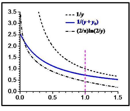
Figure 8: (Color online) The dimensionless function (134) with the zero-field cutoff parameter (135). See text for details.

Figure 8 shows the zero-field behavior of the $\Phi(y)$ function as compared to the corresponding $\Phi_{1}(y)$ and $\Phi_{2}(y)$ functions. We see that $\Phi(y)$ gradually approaches $\Phi_{2}(y)=1/y$ for increasing $y>1$. For decreasing $y<1$, on the other hand, $\Phi(y)$ is very close to the logarithmic behavior as given by $\Phi_{1}(y)$, with the exception that there is no divergence at $y\sim 0$ due to the presence of the cutoff. The cutoff parameter (135) is field dependent, decreasing as the field grows, which is consistent with the behavior of the original potential (133). Multiplying Eq. (134) by the dimensional factor $-e^{2}/2R_{CN}\epsilon$ and putting $y=|z|/2R_{CN}$, we obtain the attractive longitudinal cusp-type cutoff potential (31) we build our analysis on in this paper.

References

- (1) R.Saito, G.Dresselhaus, and M.S.Dresselhaus, Science of Fullerens and Carbon Nanotubes (Imperial College Press, London, 1998).
- (2) H.Dai, Surf. Sci. 500, 218 (2002).
- (3) L.X.Zheng, M.J.O’Connell, S.K.Doorn, X.Z.Liao, Y.H. Zhao, E.A.Akhadov, M.A.Hoffbauer, B.J.Roop, Q.X.Jia, R.C.Dye, D.E.Peterson, S.M.Huang, J.Liu and Y.T.Zhu, Nature Materials 3, 673 (2004).
- (4) S.M.Huang, B.Maynor, X.Y.Cai, and J.Liu, Advanced Materials 15, 1651 (2003).
- (5) R.H.Baughman, A.A.Zakhidov, and W.A.de Heer, Science 297, 787 (2002).
- (6) A.Popescu, L.M.Woods, and I.V.Bondarev, Nanotechnology 19, 435702 (2008).
- (7) J.E.Trancik, S.C.Barton, and J.Hone, Nano Lett. 8, 982 (2008).
- (8) I.V.Bondarev and B.Vlahovic, Phys. Rev. B 74, 073401 (2006).
- (9) I.V.Bondarev and B.Vlahovic, Phys. Rev. B 75, 033402 (2007).
- (10) I.V.Bondarev, J. Electron. Mater. 36, 1579(2007).
- (11) I.V.Bondarev, Optics & Spectroscopy (Springer) 103, 366 (2007).
- (12) H.Shimoda, B.Gao, X.P.Tang, A.Kleinhammes, L.Fleming, Y.Wu, and O.Zhou, Phys. Rev. Lett. 88, 015502 (2001).
- (13) G.-H. Jeong, A.A.Farajian, R.Hatakeyama, T.Hirata, T.Yaguchi, K.Tohji, H.Mizuseki, and Y.Kawazoe, Phys. Rev. B 68, 075410 (2003)
- (14) G.-H.Jeong, A.A.Farajian, T.Hirata, R.Hatakeyama, K. Tohji, T.M.Briere, H.Mizuseki, and Y.Kawazoe, Thin Solid Films 435, 307 (2003).
- (15) M.Khazaei, A.A.Farajian, G.-H.Jeong, H.Mizuseki, T. Hirata, R.Hatakeyama, and Y.Kawazoe, J. Phys. Chem. B 108, 15529 (2004).
- (16) A.Högele, Ch.Galland, M.Winger, and A.Imamolu, Phys. Rev. Lett. 100, 217401 (2008).
- (17) T.G.Pedersen, Phys. Rev. B 67, 073401 (2003).
- (18) T.G.Pedersen, Carbon 42, 1007 (2004).
- (19) R.B.Capaz, C.D.Spataru, S.Ismail-Beigi, and S.G.Louie, Phys. Rev. B 74, 121401(R) (2006).
- (20) C.D.Spataru, S.Ismail-Beigi, L.X.Benedict, and S.G. Louie, Phys. Rev. Lett. 92, 077402 (2004).
- (21) F.Wang, G.Dukovic, L.E.Brus, and T.F.Heinz, Phys. Rev. Lett. 92, 177401 (2004).
- (22) F.Wang, G.Dukovic, L.E.Brus, and T.F.Heinz, Science 308, 838 (2005).
- (23) A.Hagen, M.Steiner, M.B.Raschke, C.Lienau, T.Hertel, H.Qian, A.J.Meixner, and A.Hartschuh, Phys. Rev. Lett. 95, 197401 (2005).
- (24) F.Plentz, H.B.Ribeiro, A.Jorio, M.S.Strano, M.A.Pimenta, Phys. Rev. Lett. 95, 247401 (2005).
- (25) F.Xia, M.Steiner, Y.-M.Lin, and Ph.Avouris, Nature Nanotechnology 6, 609 (2008).
- (26) B.F.Habenicht and O.V.Prezhdo, Phys. Rev. Lett. 100, 197402 (2008).
- (27) V.Perebeinos, J.Tersoff, and Ph.Avouris, Phys. Rev. Lett. 94, 027402 (2005).
- (28) M.Lazzeri, S.Piscanec, F.Mauri, A.C.Ferrari, and J.Robertson, Phys. Rev. Lett. 95, 236802 (2005).
- (29) S.Piscanec, M.Lazzeri, J.Robertson, A.C.Ferrari, and F. Mauri, Phys. Rev. B 75, 035427 (2007).
- (30) S.Zaric, G.N.Ostojic, J.Shaver, J.Kono, O.Portugall, P.H.Frings, G.L.J.A.Rikken, M.Furis, S.A.Crooker, X. Wei, V.C.Moore, R.H.Hauge, and R.E.Smalley, Phys. Rev. Lett. 96, 016406 (2006).
- (31) V.Perebeinos and Ph.Avouris, Nano Lett. 7, 609 (2007).
- (32) A.Srivastava, H.Htoon, V.I.Klimov, and J.Kono, Phys. Rev. Lett. 101, 087402 (2008).
- (33) M.S.Dresselhaus, G.Dresselhaus, R.Saito, and A.Jorio, Annu. Rev. Phys. Chem. 58, 719 (2007).
- (34) T.Pichler, M.Knupfer, M.S.Golden, J.Fink, A.Rinzler, and R.E.Smalley, Phys. Rev. Lett. 80, 4729 (1998).
- (35) C.D.Spataru, S.Ismail-Beigi, R.B.Capaz, and S.G.Louie, Phys. Rev. Lett. 95, 247402 (2005).
- (36) Y.-Z.Ma, C.D.Spataru, L.Valkunas, S.G.Louie, and G.R. Fleming, Phys. Rev. B 74, 085402 (2006).
- (37) J.Bellessa, C.Bonnand, J.C.Plenet, and J.Mugnier, Phys. Rev. Lett. 93, 036404 (2004).
- (38) W.Zhang, A.O.Govorov, and G.W.Bryant, Phys. Rev. Lett. 97, 146804 (2006).
- (39) Y.Fedutik, V.V.Temnov, O.Schöps, U.Woggon, and M.V. Artemyev, Phys. Rev. Lett. 99, 136802 (2007).
- (40) I.V.Bondarev, G.Ya.Slepyan and S.A.Maksimenko, Phys. Rev. Lett. 89, 115504 (2002).
- (41) I.V.Bondarev and Ph.Lambin, Phys. Rev. B 70, 035407 (2004).
- (42) I.V.Bondarev and Ph.Lambin, Phys. Lett. A 328, 235 (2004).
- (43) I.V.Bondarev and Ph.Lambin, Solid State Commun. 132, 203 (2004).
- (44) I.V.Bondarev and Ph.Lambin, Phys. Rev. B 72, 035451 (2005).
- (45) I.V.Bondarev and Ph.Lambin, in: Trends in Nanotubes Reasearch (Nova Science, NY, 2006). Ch.6, pp.139-183.
- (46) W.Vogel and D.-G.Welsch, Quantum Optics (Wiley-VCH, NY, 2006). Ch.10, p.337.
- (47) L.Knöll, S.Scheel, and D.-G.Welsch, in: Coherence and Statistics of Photons and Atoms, edited by J.Peřina (Wiley, NY, 2001).
- (48) S.Y.Buhmann and D.-G.Welsch, Prog. Quantum Electron. 31, 51 (2007).
- (49) L.X.Benedict, S.G.Louie, and M.L.Cohen, Phys. Rev. B 52, 8541 (1995).
- (50) S.Tasaki, K.Maekawa, and T.Yamabe, Phys. Rev. B 57, 9301 (1998).
- (51) Z.M.Li, Z.K.Tang, H.J.Liu, N.Wang, C.T.Chan, R.Saito, S.Okada, G.D.Li, J.S.Chen, N.Nagasawa, and S.Tsuda, Phys. Rev. Lett. 87, 127401 (2001).
- (52) A.G.Marinopoulos, L.Reining, A.Rubio, and N.Vast, Phys. Rev. Lett. 91, 046402 (2003).
- (53) T.Ando, J. Phys. Soc. Jpn. 74, 777 (2005).
- (54) B.Kozinsky and N.Marzari, Phys. Rev. Lett. 96, 166801 (2006).
- (55) H.Haken, Quantum Field Theory of Solids, (North-Holland, Amsterdam, 1976).
- (56) S.Uryu and T.Ando, Phys. Rev. B 74, 155411 (2006).
- (57) L.D.Landau and E.M.Lifshits, The Classical Theory of Fields (Pergamon, New York, 1975).
- (58) K.Kempa and P.R.Chura, special edition of the Kluwer Academic Press Journal, edited by L.Liz-Marzan and M.Giersig (2002).
- (59) K.Kempa, D.A.Broido, C.Beckwith, and J.Cen, Phys. Rev. B 40, 8385 (1989).
- (60) A.S.Davydov, Quantum Mechanics (Pergamon, New York, 1976).
- (61) V.N.Popov, L.Henrard, Phys. Rev. B 70, 115407 (2004).
- (62) M.F.Lin, D.S.Chuu, and K.W.-K.Shung, Phys. Rev. B 56, 1430 (1997).
- (63) H.Ehrenreich and M.H.Cohen, Phys. Rev. 115, 786 (1959).
- (64) X.Blase, L.X.Benedict, E.L.Shirley, and S.G.Louie, Phys. Rev. Lett. 72, 1878 (1994).
- (65) K.Kempa, Phys. Rev. B 66, 195406 (2002).
- (66) E.Hanamura, Phys. Rev. B 38, 1228 (1988).
- (67) J.P.Reithmaier, G.Sȩk, A.Löffler, C.Hofmann, S.Kuhn, S.Reitzenstein, L.V.Keldysh, V.D.Kulakovskii, T.L.Reinecke, and A.Forchel, Nature 432, 197 (2004).
- (68) T.Yoshie, A.Scherer, J.Hendrickson, G.Khitrova, H.M. Gibbs, G.Rupper, C.Ell, O.B.Shchekin, and D.G.Deppe, Nature 432, 200 (2004).
- (69) E.Peter, P.Senellart, D.Martrou, A.Lemaître, J.Hours, J.M.Gérard, and J.Bloch, Phys. Rev. Lett. 95, 067401 (2005).
- (70) D.A.B.Miller, D.S.Chemla, T.C.Damen, A.C.Gossard, W.Wiegmann, T.H.Wood, and C.A.Burrus, Phys. Rev. Lett. 53, 2173 (1984).
- (71) D.A.B.Miller, D.S.Chemla, T.C.Damen, A.C.Gossard, W.Wiegmann, T.H.Wood, and C.A.Burrus, Phys. Rev. B 32, 1043 (1985).
- (72) A.Zrenner, E.Beham, S.Stufler, F.Findeis, M.Bichler, and G.Abstreiter, Nature 418, 612 (2002).
- (73) H.J.Krenner, E.C.Clark, T.Nakaoka, M.Bichler, C.Scheurer, G.Abstreiter, and J.J.Finley, Phys. Rev. Lett. 97, 076403 (2006).
- (74) In real CNs, the existence of two equivalent energy valleys in the 1st Brillouin zone, the - and -valleys with opposite electron helicities about the CN axis, results into dark and bright excitonic states in the lowest energy spin-singlet manifold AndoDarkExciton . Since the electric interaction does not involve spin variables, both - and -valleys are affected equally by the electrostatic field in our case, and the detailed structure of the exciton wave function multiplet is not important. This is opposite to the non-zero magnetostatic field case where the field affects the - and -valleys differently either to brighten the dark excitonic states Srivastava , or to create Landau sublevels Ando for longitudinal and perpendicular orientation, respectively.
- (75) T.Ando, J. Phys. Soc. Jpn. 75, 024707 (2006).
- (76) T.Ogawa and T.Takagahara, Phys. Rev. B 44, 8138 (1991).
- (77) A.Jorio, C.Fantini, M.A.Pimenta, R.B.Capaz, Ge.G.Samsonidze, G.Dresselhaus, M.S.Dresselhaus, J.Jiang, N. Kobayashi, A.Grüneis, and R.Saito, Phys. Rev. B 71, 075401 (2005).
- (78) We are based on the zero-exciton-temperature approximation in here Suna , which is well justified because of the exciton excitation energies much larger than in CNs. The exciton Hamiltonian (4) does not require the thermal averaging over the exciton degrees of freedom then, yielding the temperature independent total exciton energy (6). One has to keep in mind, however, that the exciton excitation energy can be affected by the enviromental effect not under consideration in here (see Ref. Miyauchi ).
- (79) A.Suna, Phys. Rev. 135, A111 (1964).
- (80) Y.Miyauchi, R.Saito, K.Sato, Y.Ohno, R.Iwasaki, T.Mizutani, J.Jiang, and S.Maruyama, Chem. Phys. Lett. 442, 394 (2007).
- (81) I.V.Bondarev, Y.Nagai, M.Kakimoto, T.Hyodo, Phys. Rev. B 72, 012303 (2005).
- (82) J.D.Jackson, Classical Electrodynamics (Wiley, New York, 1975).
- (83) Higher Transcendental Functions, edited by H.Bateman and A.Erdélyi (Mc Graw-Hill, New York, 1955). Vol. 3.
- (84) Handbook of Mathematical Functions, edited by M.Abramovitz and I.A.Stegun (Dover, New York, 1972).
- (85) L.D.Landau and E.M.Lifshits, Quantum Mechanics: Non-Relativistic Theory (Pergamon, New York, 1977).
- (86) S.Liu, J.Li, Q.Shen, Y.Cao, X.Guo, G.Zhang, C.Feng, J.Zhang, Z.Liu, M.L.Steigerwald, D.Xu, and C.Nuckolls, Angew. Chem. 48, 4759 (2009).
- (87) P.L.Hernndes-Martinez and A.O.Govorov, Phys. Rev. B 78, 035314 (2008).
- (88) H.Qian, C.Georgi, N.Anderson, A.A.Green, M.C.Hersam, L.Novotny, and A.Hartschuh, Nano Lett. 8, 1363 (2008).
- (89) P.H.Tan, A.G.Rozhin, T.Hasan, P.Hu, V.Scardaci, W.I.Milne, and A.C.Ferrari, Phys. Rev. Lett. 99, 137402 (2007).
- (90) H.Hirori, K.Matsuda, and Y.Kanemitsu, Phys. Rev. B 78, 113409 (2008).