Abstract. A set of traveling wave solution to convection-reaction-diffusion equation is studied by means of methods of local nonlinear analysis and numerical simulation. It is shown the existence of compactly supported solutions as well as solitary waves within this family for wide range of parameter values.

PACS codes: 02.30.Jr; 47.50.Cd; 83.10.Gr

Keywords: convection–reaction–diffusion equation, traveling waves, symmetry rediction, dynamical system, Andronov–Hopf bifurcation, homoclinic bifurcation, solitary waves, compactons

1 Introduction

We consider evolutionary equation

$$u_{t}+u\,u_{x}-\kappa\,\left(u^{n}\,u_{x}\right)_{x}=\left(u-U_{1}\right)\,\varphi(u),$$ (1)

where $\kappa,\,\,\,U_{1}$ are positive constants, $\varphi(u)$ is a smooth function nullifying at the origin and maintaining a constant sign within the set $\left(0,\,k\,U_{1}\right)$ for some $k>1$. Equation (1) referred to as convection–reaction–diffusion equation is used for simulating transport phenomena in active media. Due to its practical applicability and a number of unusual features, equation (1) was intensely studied in recent decades [1, 2, 3, 4, 5, 6, 7, 8].

Present investigations are mainly devoted to qualitative and numerical study of the family of traveling wave (TW) solution to equation (1). Our aim is to show that under certain conditions the set of TW solutions contains periodic regimes, solitary waves and compactons with special emphasis put on the existence of compactons. Solitary wave solutions (or solitons) are exponentially localized wave packs moving with constant velocity without change of their shape. They are mostly associated with the famous Korteveg de Vries (KdV) equation and members of KdV hierarchy having the form

$$K(m)=u_{t}+u^{m}\,u_{x}+u_{xxx}=0,\qquad m\geq 1.$$ (2)

For $m=1$ solitary wave solution to KdV is as follows [9]:

$$u(t,\,x)=U(\xi)\equiv U(x-V\,t)=\frac{3\,V}{\cosh\left(\frac{\sqrt{V}}{2}\,\xi\right)},$$

where $V$ stands for the wave pack velocity.

In 1993 Philip Rosenau and John Hyman put forward the following generalization to KdV hierarchy [10]:

$$K(m,\,n)=u_{t}+\left(u^{m}\right)_{x}+\left(u^{n}\right)_{xxx}=0,\qquad m,\,n\geq 2.$$ (3)

Modification in the higher-derivative term causes that members of $K(m,\,n)$ hierarchy possess solutions with compact support. For $m=n=2$ compactly supported solution (or compacton) has the form

$$u(t,\,x)=U(\xi)\equiv U(x-V\,t)=\left\{\begin{array}[]{c}\frac{4\,V}{3}\,\cos^{2}\left[\frac{x-V\,t}{4}\right]\quad\mbox{if}\quad\left|\frac{x-V\,t}{4}\right|\\ 0\quad\mbox{otherwise}.\end{array}\right.$$

Both solitons and compactons are the TW solutions, depending in fact on a single variable $\xi=x-V\,t$, are described by ODEs appearing when the TW ansatz $u(t,\,x)=U(\xi)$ is inserted into the source equations (for details see e.g. [11]). Therefore it is possibile to give a clear geometric interpretation of solitons and compactons. To both of them correspond homoclinic trajectories in the phase space of the factorized equations. The main difference between the solitary wave and compacton is that the first one is nonzero for any $\xi$ while the last one is nonzero only upon some compact set. This is because the soliton corresponds to the homoclinic loop usually bi-asymptotic to a simple saddle. Hence the ”time” needed to penetrate the close loop is infinite. Compacton corresponds to the homoclinic loop bi-asymptotic to a topological saddle lying on a singular line. A consequence of this is that the corresponding vector field does not tend to zero as the homoclinic trajectory approaches the stationary point, hence the ”time” required to penetrate the trajectory remains finite. Let us note that the compacton in fact is a conjunction of the nonzero part corresponding to the homoclinic loop and the trivial constant solution represented by the saddle point [11].

For the sake of brevity we maintain the notation traditionally used in more specific sense. Thus, soliton is usually associated with the localized invariant solution to any completely integrable PDE, possessing a number of unusual features [9]. Some of these features are inherited by compactons as well [10, 12, 13]. Here we maintain this notion to those solutions to (1), which manifest similar geometric features as ”true” wave patterns known under these names, not pretending that they inherit all features of their famous precursors.

The structure of the article is following. In section 2 we present the dynamical system describing the TW solutions to (1) and make its qualitative analysis, obtaining conditions that contribute to the homoclinic loop appearance. At the end of this section we formulate the conditions enabling to make a distinction between compactons and solitons. Conditions formulated in section 2 contribute but not guarantee the homoclinic loop appearance. The following section contains the results of numerical simulations revealing that expected scenarios of solitons’ and compactons’ appearance really take place. In section 4 we perform a brief discussion of the results obtained and outline directions of further investigations.

2 Factorized system and its qualitative analysis

2.1 Statement of the problem

We are going to analyze the set of TW solutions to (1), described by the following formula:

$$u(t,\,x)=U(\xi)\equiv U\left(x-V\,t\right).$$ (4)

Inserting ansatz (4) into the GBE one can obtain, after some manipulation, the following dynamical system:

$$\Delta(U)\,\dot{U}=\Delta(U)\,W,$$ (5)

$$\Delta(U)\,\dot{W}=\varphi(U)\left(U_{1}-U\right)-\kappa\,n\,U^{n-1}\,W^{2}+\left(U-V\right)\,W,$$

where $\Delta(U)=\kappa\,U^{n}$. We are going to formulate the conditions contributing to soliton-like and compacton-like solutions to equation (1) by analyzing the factorized system (5). Let us note that in the case of both KdV and $K(m,\,n)$ hierarchies’ members the procedure of factorization lead to the Hamiltonian dynamical systems for which distinguishing the presence of homoclinic loops is more or less trivial [11]. The situation with system (5) is not so simple since it is not Hamiltonian. And we cannot expect that the homoclinic loops will form a one-parametric family as this is the case with the Hamiltonian systems. Contrary, the homoclinic loop in our case can appear as a result of one or several successive bifurcations taking place at specific values of the parameters. Let us stress that existence of the homoclinic loop corresponding to compacton is possible due to the presence of the factor $\Delta(U)$ at the LHS of system (5). Since the function $\Delta(U)$ contains the origin, which is the stationary point of system (5), then the natural way of proceedings is following. We state the condition that guarantee the appearance of the stable limit cycle in proximity of the stationary point $(U_{1},\,0)$, and ensure that simultaneously the stationary point $(0,\,0)$ is a saddle and remain so as the parameter of bifurcation is changed. By proper change of the bifurcation parameter we can cause the growth of size of the limit cycle and in presence of near-by saddle it finally could give way to the homoclinic bifurcation. Since the latter bifurcation is nonlocal, we cannot trace its appearance using the methods of local nonlinear analysis, as this is the case with Andronov-Hopf bifurcation. Therefore on the final step we are forced to resort to numerical simulations. And of course answer the question on whether the homoclinic loop corresponds to compacton-like solution or not needs special treatment based upon the asymptotic analysis. This and other issues are analyzed in the following subsections.

2.2 Andronov-Hopf bifurcation in system (5)

To formulate the conditions which guarantee the stable limit cycle appearance in vicinity of the stationary point $(U_{1},\,0)$, let us consider the Jacobi matrix

$$J_{1}=\left(\begin{array}[]{cc}0&\Delta(U_{1})\\ -{\varphi}(U_{1})&U_{1}-V.\end{array}\right).$$

corresponding to this point. In order that $(U_{1},\,0)$ be a center, the eigenvalues of $J_{1}$ should be pure imaginary and this is so when the following conditions are fulfilled:

$$\mbox{Trace}\,{J_{1}}=U_{1}-V=0,$$ (6)

$$\mbox{Det}\,{J_{1}}=\Delta(U_{1})\varphi(U_{1})>0$$ (7)

The first condition immediately gives us the critical value of the wave pack velocity $V_{cr}=U_{1}.$ The second one is equivalent to the statement that $\varphi(U_{1})$ is positive.

The next thing we are going to do is a study of the stability of limit cycle appearing. As is well known [14, 15], this is the real part of the first Floquet index $\Re{C_{1}}$ that determines whether the cycle is stable or not.

For $\Delta(U_{1})=\kappa U_{1}^{n}>0$ condition $\Re{C_{1}}<0$ assures that the limit cycle, appearing in system when $V<V_{cr}$, will be stable.

To obtain the expression for $\Re{C_{1}}$, the standard formula contained e.g. in [15] could be applied providing that system in vicinity of the center is presented in the form

$$\left(\begin{array}[]{c}\dot{z}_{1}\\ \dot{z}_{2}\end{array}\right)=\left(\begin{array}[]{lc}0&-\Omega\\ \Omega&0\end{array}\right)\cdot\left(\begin{array}[]{c}z_{1}\\ z_{2}\end{array}\right)+\left(\begin{array}[]{c}F(z_{1},z_{2})\\ G(z_{1},z_{2})\end{array}\right),$$ (16)

where $\Omega=\sqrt{\mu\cdot\nu},$ $\mu=\Delta(U_{1})$, $\nu=\varphi(U_{1})$, $F(z_{1},z_{2})$ and $G(z_{1},z_{2})$ contain all nonlinear terms. In this (canonical) representation the real part of the Floquet index $\Re\,C_{1}$ is expressed by the following formula [15]:

$$16\,\Re\,C_{1}=F_{111}+F_{122}+G_{112}+G_{222}+\frac{1}{\Omega}\left\{F_{12}\left(F_{11}+F_{22}\right)-\right.$$

$$\left.-G_{12}\,\left(G_{11}+G_{22}\right)-F_{11}\,G_{11}+F_{22}\,G_{22}\right\}.$$ (17)

Here $F_{ijk},\,\,F_{ij}$ stand for the coefficients of the function’s $F(z_{1},z_{2})$ monomials $z_{i}\,z_{j}\,z_{k}$, $z_{i}\,z_{j}$ correspondingly. Similarly, indices $G_{ijk},\,\,G_{ij}$ correspond to the function’s $G(z_{1},z_{2})$ monomials’ coefficients.

Assuming that relations (6)–(7) are satisfied, let us rewrite system (5 ) in coordinates $y_{1}=U-U_{1},\,\,y_{2}=W$:

$$\Delta(U)\frac{d}{d\,\xi}\left(\begin{array}[]{c}y_{1}\\ y_{2}\end{array}\right)=\left(\begin{array}[]{lc}0&\mu\\ -\,\nu&0\end{array}\right)\left(\begin{array}[]{c}y_{1}\\ y_{2}\end{array}\right)+\left(\begin{array}[]{c}\Phi_{1}(y_{1},\,y_{2})\\ \Phi_{2}(y_{1},\,y_{2})\end{array}\right),$$ (18)

where $\Phi_{1}(y_{1},\,y_{2}),\,\,\Phi_{2}(y_{1},\,y_{2})$ are nonlinear terms which are as follows:

$$\Phi_{1}(y_{1},\,y_{2})=\kappa nU_{1}^{n-2}\,y_{1}\,y_{2}\left(U_{1}+\frac{n-1}{2}y_{1}\right)+O\left(|y_{i}|^{4}\right),\qquad\qquad\qquad$$ (19)

$$\Phi_{2}(y_{1},\,y_{2})=-\left\{\kappa\,U_{1}^{n-1}y_{2}^{2}+n(n-1)\kappa\,U_{1}^{n-2}y_{1}\,y_{2}^{2}+\qquad\qquad\qquad\qquad\qquad\right.$$ (20)

$$\left.+y_{1}\left[\dot{\varphi}\left(U_{1}\right)\,y_{1}+\frac{1}{2}\ddot{\varphi}\left(U_{1}\right)\,y_{1}^{2}-y_{2}\right]\right\}+O\left(|y_{i}|^{4}\right).$$

A passage to canonical variables $(z_{1},\,z_{2})$ can be attained by means of transformation

$$\left(\begin{array}[]{c}z_{1}\\ z_{2}\end{array}\right)=\left(\begin{array}[]{lc}-\sqrt{\nu}&0\\ 0&\sqrt{\mu}\end{array}\right)\cdot\left(\begin{array}[]{c}y_{1}\\ y_{2}\end{array}\right),$$

This gives us the canonical system (16) with

$$F(z_{1},z_{2})=\frac{\kappa\,n\,U_{1}^{n-2}}{\Omega}z_{1}\,z_{2}\,\left[\sqrt{\nu}\,U_{1}-\frac{n-1}{2}z_{1}\right]+O(|z_{i}|^{4}),$$ (22)

$$G(z_{1},z_{2})=-\frac{\mu}{2\,\nu\Omega}z_{1}^{2}\left[2\,\dot{\varphi}(U_{1})\sqrt{\nu}-\,{\ddot{\varphi}(U_{1})}z_{1}\right]-\,\frac{\sqrt{\mu}}{\Omega}{z_{1}\,z_{2}}+\qquad\qquad\qquad$$

$$+\frac{\kappa\,n\,U_{1}^{n-2}}{\Omega}z_{2}^{2}\left[(n-1)\,z_{1}-U_{1}\sqrt{\nu}\right]+O(|z_{i}|^{4}).\qquad\qquad\qquad$$

Analysis of the formulae (2.2), (22) shows that the function $F(z_{1},z_{2})$ does not contribute to the real part of the Floquet index, which in our case is expressed as follows:

$$\Re{C_{1}}=-\frac{1}{16\,\Omega}\,G_{12}\,\left(G_{11}+G_{22}\right)=-\,\frac{1}{16\,\Omega^{2}\,\varphi(U_{1})}\left\{\Delta(U_{1})\,\dot{\varphi}(U_{1})+\kappa\,n\varphi(U_{1})\,U_{1}^{n-1}\right\}.$$

So the following statement holds.

Theorem 1. If the inequality

$$U_{1}\,\dot{\varphi}(U_{1})+n\varphi(U_{1})\,>\,0$$ (23)

is fulfilled then in some vicinity of the critical value of the wave pack velocity $V_{cr}=U_{1}$ a stable limit cycle exists.

2.3 Study of the stationary point $(0,\,0)$

From now on we shall investigate system with $\varphi(U)=U^{m}$:

$$\Delta(U)\,\dot{U}=\Delta(U)\,W,$$ (24)

$$\Delta(U)\,\dot{W}=\varphi(U)\left(U_{1}-U\right)-\kappa\,n\,U^{n-1}\,W^{2}+\left(U-V\right)\,W,$$

Our next step is to state the conditions assuring that the stationary point $(0,0)$ is a topological saddle or at least contains a saddle sector in the right half-plane. The standard theory [16] can be applied for this purpose. Our system can be written down in the form

$$\frac{d}{d\,T}\left(\begin{array}[]{c}U\\ W\end{array}\right)=\left(\begin{array}[]{lc}0&0\\ U_{1}\,\dot{\varphi}(0)&-V\end{array}\right)\left(\begin{array}[]{c}U\\ W\end{array}\right)+\mbox{nonl.\,\,terms},$$ (25)

where $\frac{d}{d\,T}=\kappa\,U^{n}\,\frac{d}{d\,\xi}$ and since the trace of its linearization matrix is nonzero then the analysis prescribed in Chapter IX of [16] for this type of a complex stationary points is the following.

1. Find the change of variables $\left(U,\,W,\,T\right)\mapsto\left(x,\,y,\,\tau\right)$ enabling to write down system (25) in the standard form

   $$\frac{d\,x}{d\,\tau}=P_{2}\left(x,\,y\right),$$

   $$\frac{d\,y}{d\,\tau}=y+Q_{2}\left(x,\,y\right),$$

   where $P_{2}\left(x,\,y\right)$, $Q_{2}\left(x,\,y\right)$ are polynomials of degree 2 or higher.

2. Solve the equation $y+Q_{2}\left(x,\,y\right)=0$ with respect to y, presenting result in the form of the asymptotic decomposition $y=\varphi(x)=\alpha_{1}\,x^{\mu_{1}}+\alpha_{2}\,x^{\mu_{2}}+...$.

3. Find the asymptotic decomposition

   $$P_{2}\left(x,\,\varphi(x)\right)=\Delta_{m}\,x^{m}+....$$

4. Depending on the values of $m$ and the sign of $\Delta_{m}$ select the type of the complex stationary point using the theorem 65 from [16].

5. Return to the original variables $\left(U,\,W,\,T\right)$ and analyze on whether the geometry of the problem allows for the homoclinic bifurcation appearance.

So let us present results obtained for system (24). The case $m>1$ is most simple for analyzing since the canonical system is obtained by the formal change $\left(U,\,W\right)\mapsto\left(x,\,y\right)$ and passage to new independent variable $\tau=-V\,T$. As a result we get the following system:

$$\frac{d\,x}{d\,\tau}=-\frac{\kappa}{V}x^{n}\,y,=P_{2}(x,\,y),$$ (26)

$$\frac{d\,y}{d\,\tau}=y-\frac{1}{V}\left\{xy-\kappa\,n\,x^{n-1}\,y^{2}-x^{m}\,\left(x-U_{1}\right)\right\}=y+Q_{2}(x,\,y).$$

Presenting $y$ in the form of series $y=\alpha_{1}\,x^{\mu}_{1}+...$ and solving the equation $y+Q_{2}(x,\,y)=0,$ we obtain $y=\varphi(x)=\frac{U_{1}}{V}x^{m}+...$. Inserting function $\varphi(x)$ into the RHS of the first equation we get

$$P_{2}(x,\,\varphi(x))=\Delta_{n+m}x^{n+m}+...=-\kappa\,U_{1}\,x^{n+m}+....$$

Case $m=1$ is different from the previous one. Passage to canonical system is attained by means of the following transformation:

$$x=U,\quad y=W-\frac{U_{1}}{V}\,U,\quad\tau=-V\,T.$$

In new variables system read as follows:

$$\frac{d\,x}{d\,\tau}=-\frac{\kappa}{V}x^{n}\,\left(\frac{U_{1}}{V}x+y\right)=P_{2}(x,\,y),\qquad$$ (27)

$$\frac{d\,y}{d\,\tau}=y-\frac{1}{V}\left\{x\left(\frac{U_{1}}{V}x+y\right)-\kappa\,n\,x^{n-1}\,\left(\frac{U_{1}}{V}x+y\right)^{2}-x^{2}+U_{1}\,P_{2}(x,\,y)\right\}=$$

$$=y+Q_{2}(x,\,y).$$

Solving equation $y+Q_{2}(x,\,y)=0,$ we get $y=\varphi(x)=a_{2}\,x^{2}+...$, where index $a_{2}$ depends upon $n$ Inserting function $\varphi(x)$ into the RHS of the first equation we get

$$P_{2}(x,\,\varphi(x))=\Delta_{n+1}x^{n+1}+...=-\kappa\,U_{1}\,x^{n+1}+....$$

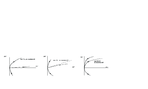
Figure 1: Phase portraits in vicinity of $(0,\,0)$ for different values of the parameter $m$

The last case we are going to analyze is that with $m=\frac{1}{2}$. The motivation of such a choice will be clear later on. In order that the analytical theory be applicable we make a change variables $Z=\sqrt{U}$. After that we get the system

$$\frac{d\,Z}{d\,T}=-\frac{\kappa}{2}Z^{2\,n-1}\,W,$$ (28)

$$\frac{d\,W}{d\,T}=W\left(Z^{2}-V\right)-\kappa\,n\,Z^{2(n-1)}W^{2}+Z\,\left(U_{1}-Z^{2}\right).$$

Passage to the canonical variables is performed by the change of variables

$$x=Z,\quad y=W-\frac{U_{1}}{V}Z,\quad\tau=-D\,T.$$

The system resulting from this will be as follows:

$$\frac{d\,x}{d\,\tau}=-\frac{\kappa}{2\,V}x^{2n-1}\,\left(\frac{U_{1}}{V}x+y\right)=P_{2}(x,\,y),$$ (29)

$$\frac{d\,y}{d\,\tau}=y-\frac{1}{V}\left\{x^{2}\left(\frac{U_{1}}{V}x+y\right)-\kappa\,n\,x^{2(n-1)}\,\left(\frac{U_{1}}{V}x+y\right)^{2}-x^{3}+U_{1}\,P_{2}(x,\,y)\right\}=$$

$$=y+Q_{2}(x,\,y).$$

Solving first equation $y+Q_{2}(x,\,y)$ with respect to $y$ and inserting the function $\varphi(x)$ obtained this way into $P_{2}$ we get the decomposition

$$P_{2}(x,\,\varphi(x))=\Delta_{2n}\,x^{2n}+...=-\frac{\kappa}{2\,V}x^{2n}+...$$

Using the classification given in [16] we are now able to formulate the following result.

Theorem 2.

1. If $m+n$ is an odd natural number then the origin of system (26) is a topological saddle having a pair of separatrices tangent to the vertical axis and the other pair tangent to the horizontal axis when $m>1$ and to the line $W=\frac{U_{1}}{V}\,U$ when $m=1$. For even $m+n$ the stationary point is a saddle-node with two saddle sectors lying in the right half-plane. Two of its three separatrices are tangent to the vertical axis while the remaining one is tangent to the horizontal axis in case when $m>1$ and and to the line $W=\frac{U_{1}}{V}\,U$ when $m=1$. The nodal sector lying in the left half-plane is unstable.

2. If $n$ is an odd number then the origin of system corresponding to (27) is a topological saddle identical with that of the previous case. For even $n$ the stationary point is a saddle-node identical with that of the previous case

3. For any $n\geq 1$ the origin of system (29) is a saddle-node geometrically identical with that from the previous two cases.

The crucial fact appearing from this analysis is that the stationary points $(0,\,0)$ of the canonical systems (26)–(29) depending on the values of the parameters $m,\,n$ are either saddles or saddle-nodes with the saddle sectors placed at the right half-space. The return to the original coordinates does not cause the change the position of the saddle sectors but changes the orientation of vector fields and the angle at which the outgoing separatrice leaves the stationary point. The local phase portraits corresponding to three distinct cases are shown on figure 1 reconstructed on the basis if the analysis of relation between (26)–(29) and system (24).

Before we start to discuss the results of numerical study of system (24), let us consider the question on when the presumably appearing homoclinic loop corresponds to the compacton-like solution to the source equation (1). To answer this question we are going to find the solution $W(U)=\alpha_{1}\,U^{\mu_{1}}+\alpha_{2}\,U^{\mu_{2}}+...$ of equation

$$\kappa\,U^{n}\,W\,\frac{d\,W}{d\,U}=G\equiv U^{m}\,(U_{1}-U)-\kappa\,n\,U^{n-1}\,W^{2}-\left(V-U\right)\,W,$$ (30)

(equivalent to system (24)) up to the given order and next estimate the limit of the vertical component of vector field

$$K=\lim_{U\to 0}\frac{G\left(U,W(U)\right)}{\kappa\,U^{n}}.$$ (31)

Homoclinic loop will correspond to comactly-supported solution if K is finite or infinite and also if it tends to zero not quicker than $U^{\mu},\,\,\mbox{where}\,\,1/2<\mu<1.$

Equation (2.3) can be re-written as follows:

$$\kappa\,U^{n+2\,\mu_{1}-1}\left(\alpha_{1}+\alpha_{2}\,U^{\mu_{2}-\mu_{1}}+...\right)\,\left(\mu_{1}\,\alpha_{1}+\mu_{2}\,\alpha_{2}\,U^{\mu_{2}-\mu_{1}}+...\right)=$$

$$=U^{1+\mu_{1}}\left(\alpha_{1}+\alpha_{2}\,U^{\mu_{2}-\mu_{1}}+...\right)-V\,\left(\alpha_{1}+\alpha_{2}\,U^{\mu_{2}-\mu_{1}}+...\right)-$$ (32)

$$-\kappa\,n\,U^{n+2\,\mu_{1}-1}\left(\alpha_{1}^{2}+2\alpha_{1}\alpha_{2}\,U^{\mu_{2}-\mu_{2}}+....\right)-U^{m+1}+U_{1}\,U^{m}.$$

The procedure of solving (2.3) is pure algebraic: we collect the coefficient of different powers of $U$ end equalize them to zero. The lowest power in the RHS is either $U^{\mu_{1}}$ or $U^{\mu_{1}}$ or $U^{n+2\,\mu_{1}-1}$. The number ${n+2\,\mu_{1}-1}$ cannot be less or equal to $\mu_{1}$ because it involves the inequality $0<\mu_{1}\leq 1-n$ which is impossible for any natural $n$. On the other hand if ${n+2\,\mu_{1}-1}\leq m$ then $\mu_{1}$ becomes an ”orphan” and $\alpha_{1}$ should be nullified.

So $U^{n+2\,\mu_{1}-1}$ cannot be the lowest monomial. From this immediately appears that the only choice leading to the nontrivial solution is $\mu_{1}=m$. Next important observation is such that the first nonzero monomial at the RHS should have as a counterpart at the LHS the least monomial, that is $U^{n+2\,\mu_{1}-1}\equiv U^{n+2\,m-1}$. This in turn is sufficient to estimate the limit (31). In fact,

$$\frac{G\left(U,W(U)\right)}{\Delta(U)}=\frac{G\left(U,W(U)\right)}{\kappa\,U^{n}}=\frac{A_{1}\,U^{n+2\,m-1}+...}{\kappa\,U^{n}}\sim\frac{A_{1}}{\kappa}\,U^{2\,m-1}+...$$

And now we are ready to formulate the main result of this subsection.

Proposition 1.Homoclinic loop bi-asymptotic to stationary point $(0,\,0)$ of system (24) corresponds to compacton-like solution to the initial PDE if $m\leq\frac{1}{2}$.

Presented above result delivers sufficient but not necessary condition for the homoclinic loop corresponding to compacton. Basing on the local asymptotic analysis it is possible to show that for $0<m<1$ and any natural $n$ trajectory bi-asymptotic to stationary point $(0,\,0)$ will also correspond to compactly–supported traveling wave. The proof is somewhat cumbersome and we shall not present it here.

We would like to know, what sort of TW corresponds to the homoclinic loop in case when $m\geq 1$ and $n\geq 1$. Presently we are not able to answer this question rigorously. Nevertheless, we bring some arguments evidencing that the ”tail” of TW in this case spreads up to $-\infty$ whereas the front sharply ends. This is so because the ”tail” corresponds to the outgoing separatrix which is tangent to either horizontal axis (if $m>1$) or the line $W=\frac{U_{1}}{V}\,U$ (if $m=1$). On the other hand, the incoming separatrix enters the origin at the angle $\frac{2\,\pi}{3}$. From these observations conclusions can be made concerning the shape of TW. Corresponding arguments will be delivered for the case $m=n=1$.

Analysis of formula (27) enables to state that outgoing separatrix is tangent to the straight line $W=\frac{U_{1}}{V}\,U$. So the first coordinate of the saddle separatrix in vicinity of the origin satisfies the equation

$$\frac{d\,U}{d\,\xi}=\frac{U_{1}}{V}\,U+O\left(U^{2}\right),$$

having the approximated solution $U(\xi)\cong Aexp(\frac{U_{1}}{V}\,\xi)$. This form of approximate solution tells us that separatrix reaches the origin as $\xi\rightarrow-\infty$.

Now let us consider the incoming separatrix, which is tangent to the vertical axis and lies at the fourth quadrant. This enables us to assume that $W=-B\,U^{\sigma}+o\left(U^{\sigma}\right)$, where $0<\sigma<1$ and $B>0$. Approximate equation describing the first coordinate of incoming separatrix is then as follows

$$\frac{d\,U}{d\,\xi}=-B\,U^{\sigma}+o\left(U^{\sigma}\right).$$

Hence

$$U(\xi)\cong\left[B(1-\sigma)\,\left(\xi_{0}-\xi\right)\right]^{\frac{1}{1-\sigma}}.$$

Analysis of this formula shows that trajectory reaches reaches the origin in finite ”time”.

3 Results of numerical simulation

Numerical simulation of system (24) were carried out for different values of the parameters. Let us consider first the results of simulation obtained for $\kappa=n=1,U_{1}=3$ and $m=\frac{1}{2}$. Experiments show that at $V$ slightly less then $V_{cr}=U_{1}$ a stable limit cycle is softly created in system (24).

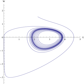
Figure 2: Phase portrait of system (24) obtained for $\kappa=n=1,U_{1}=3$, $m=\frac{1}{2}$ and $V=2.82$

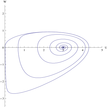
Figure 3: Homoclinic bifurcation corresponding to $\kappa=n=1,\,\,U_{1}=3$, $m=\frac{1}{2}$ and $V=2.5397975$

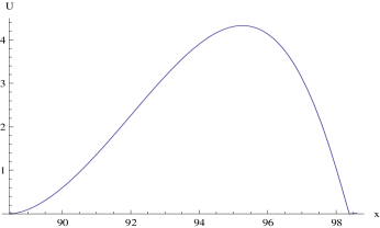
Figure 4: Compactly-supported solution of the equation (1) corresponding to $\varphi(u)=u^{\frac{1}{2}}$, $\kappa=n=1,\,\,U_{1}=3$

Its radius grows as $V$ decreases. As the left end of the periodic trajectory approaches the origin, it becomes asymmetric (fig. 2). At $V\approx 2.5397975$ periodic trajectory destroys giving way to the homoclinic bifurcation (fig. 3). Corresponding compacton-like solution to the equation (1) is shown on fig. 4. Compacton, moving from left to right, is gently sloping towards the tail. It is worth noting that the compacton-like solution is always symmetric in case it is solution to Hamiltonian system.

Another numerical simulations were put up for $\kappa=1,\,\,m=1,\,\,n=1,\,\,U_{1}=3.$ Scenario is the same as in the previous case. Limit cycle appearing at $V<U_{1}$ grows as $V$ decreases (fig. 5). Periodic trajectory is destroyed at $V\cong 2.48225$, giving way to homoclinic trajectory (fig. 6). Corresponding TW solution to source equation (1) is shown on fig. 7.

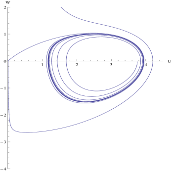
Figure 5: Phase portrait of system (24) obtained for $\kappa=m=n=1,\,\,U_{1}=3$ and $V=2.775$

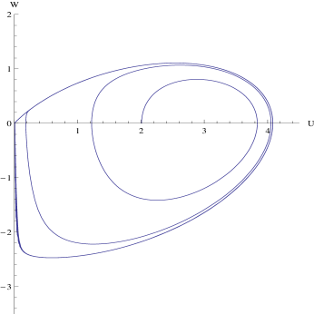
Figure 6: Homoclinic bifurcation corresponding to $\kappa=m=n=1,\,\,U_{1}=3$ and $V=2.48225$

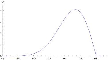
Figure 7: Solitary wave solution of the equation (1) corresponding to $\varphi(u)=u$, $\kappa=n=1,\,\,U_{1}=3$ and and $V=2.48225$

Let us finally show patterns corresponding to stronger nonlinearity of the source term. We take ${m=3}$ and the remaining parameter the same as in the previous case. Such a change leads to larger asymmetry of the homoclinic contour, fig. 8–9 and appearance of wave pattern with sharp front and very long relaxing tail, reminding shock or detonation wave, fig. 10.

Figure 8: Phase portrait of system (24) obtained for $m=3,\,\,\kappa=n=1,\,\,U_{1}=3$ and $V=2.7444875$

Figure 9: Homoclinic bifurcation corresponding to $m=3,\,\,\kappa=n=1,\,\,U_{1}=3$ and $V=2.4449$

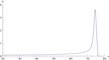
Figure 10: Solitary wave solution of the equation (1) corresponding to $\varphi(u)=u^{3}$, $\kappa=n=1,\,\,U_{1}=3$ and and $V=2.4449$

4 Final remarks

So we have shown that, depending on the values of the parameters convection-reaction-diffusion model described by equation (1) possesses compacton-like TW solutions or mixed solutions having the soliton-like tails and sharp fronts. The mere existence of compacton-like solutions is possible if the diffusion coefficient is a function of dependent variable $u$. In all cases considered wave patterns have been obtained as the result of two bifurcation. First we performed the local nonlinear analysis of dynamical system (5) describing the whole set of TW solution and stated conditions making possible the stable limit cycle creation in proximity of critical point $(U_{1},0)$. The other critical point, placed at the origin, is shown to possess simultaneously a saddle sector in the right half-plane, making possible the homoclinic loop appearance. Next we studied numerically the evolutions of periodic solutions, observing how they undergo the homoclinic bifurcation. Analytical results obtained in subsection   2.3 enable us to state when the homoclinic loop obtained in numerical experiments correspond to compacton.

The results obtained here are not completely rigorous. In particular it is rather unknown the precise value of wave pack velocity $V$ corresponding to the homoclinic bifurcation.

To obtain the solutions in question analytical methods based on the generalized symmetries [17] and related to them anasatz-based methods [18, 19, 20, 21] can be applied. Yet it is little chances to obtain them for all possible values of the parameters for the source equation is not completely integrable. So it would be desired to apply some other means, such as the rigorous computer-assisted proofs for this problem.

In connection with the results obtained a natural question arises about the benefit of solutions existing merely at selected values of the parameters. So first let us mention that the velocity of wave pack, being chosen as the bifurcation parameter, is an ”external” in some sense parameter and its value is rather connected with the portion of ”energy” delivered at the initial moment of time, which is easily controlled, while the parameters characterizing system remain unchanged.

Of prime importance is also the well known fact that invariant wave patterns such as kinks, solitons, compactons etc., very often play role of asymptotics, attracting in the long range close near-by solutions [22, 23, 11]. Study of the stability and attracting properties of the invariant solutions to (1) is very non-trivial issue going far beyond the scope of this article.

References

- [1] Tang S., Wu J., Cui M., The Nonlinear Convection–Reaction–Diffusion Equation for Modeling El Nino Events, Comm. Nonl. Sciences and Numerical Simul., vol. 1, no. 1 (1996), p. 27–35.
- [2] Korman P., Steady States and Long Time Behavior of Some Convection–Reaction–Diffusion Equations. Funcialaj Ekvacioj, vol. 40 (1997), p. 165–187.
- [3] Lou B., Singular Limits of Spatially Inhomogeneous Convection–Reaction–Diffusion Equations, Journal of Statistical Physics, vol. 129 (2007), p. 506–516.
- [4] Gilding B.,Kersner R., Travelling Waves in Nonlinear Convection–Reaction–Diffusion Equations, Springer, 2004.
- [5] Nekhamkina O., Sheintach M., Asymptotic Solutions of stationary Patterns in Convection–Reaction–Diffusion Systems, Phys Rev. E, Stat. Nonlin. Soft Matter Phys, vol. 68, no. 3 (2003), 036207.
- [6] Smoller J., Shock Waves and Reaction–Diffusion Equationss, Springer, 1994.
- [7] Cherniha R., New Ansatze and Exact Solutions for Nonlinear Reaction–Diffusion Equations, Arising in Mathematical Biology, Proc. of II Int. Conference ”Symmetry in Nonlinear Mathematical Physics, Kyiv, June 24-30, 1997”, vol. 1, 138–146.
- [8] Barannyk A., Yuryk I., Construction of Exact Solutions of Diffusion Equation, Proc. of Institute of Mathematics of NAS of Ukraine, vol. 50 (2004), Part 1, 29–33.
- [9] R.K. Dodd, J.C. Eilbek, J.D. Gibbon, H.C. Morris, Solitons and Nonlinear Wave Equations, Academic Press, London 1984.
- [10] Rosenau P. and Hyman J., Compactons: Solitons with Finite Wavelength, Phys Rev. Letter, vol. 70 (1993), No 5, 564-567.
- [11] Vladimirov V., Compacton-like solutions of the hydrodynamic system describing relaxing media , Rep. Math. Phys. 61 (2008), 381-400.
- [12] Rosenau P. and Pikovsky A., Phase Compactons in Chains of Dispersively Coupled Oscillators, Phys. Rev. Lett., vol. 94 (2005) 174102.
- [13] Pikovsky A. and Rosenau P., Phase Compactons, Physica D, vol. 218 (2006) 56–69.
- [14] Hassard B., Kazarinoff N., Wan Y.-H., Theory and Applications of Hopf Bifurcation, Cambridge Univ. Press: London, New York, 1981.
- [15] Guckenheimer J., Holmes P., Nonlinear Oscillations, Dynamical Systems and Bifurcations of Vector Fields, Springer–Verlag: New York Inc, 1987.
- [16] Andronov A., Leontovich E., Gordon I and Meyer A., Qualitative Theory of 2-nd Order Dynamical Systems, Nauka Publ., Moscow, 1976 (in Russian).
- [17] Olver P., Applications of Lie Groups to Differential Equations, Springer–Verlag: New York, Berin, Tokyo, 1996.
- [18] Fan E., Multiple Travelling Wave Solutions for Nonlinear Evolution Equations Using Symbolic Computations , Journ of Physics A: Math and Gen vol. 35 (2002), 6853–6872.
- [19] Olver P., E. Vorob’jev E., Nonclassical and Conditional Symmetries, in: CRC Handbook of Lie Group Analysis of Differential Equations, Volume III, ed. by Nail Ibragimov. - CRC Press Inc, Boca Raton, FL 1994.
- [20] Vladimirov V.A. and Kutafina E.V., Exact Travelling Wave Solutions of Some Nonlinear Evolutionary Equations , Rep. Math. Physics, vol. 54 (2004), 261–271.
- [21] Vladimirov V.A. and Kutafina E.V., Analytical description of the coherent structures within the hyperbolic generalization of Burgers equation , Rep. Math. Physics, vol.58 (2006), 465.
- [22] Barenblatt G.I., Similarity, Self-Similarity and Intermediate Asymptotics, Cambridge Univ. Press 1986.
- [23] Biler P. and Karch G.(eds.), Self-similar solutions in Nonlinear PDEs, Banach Center Publications, vol. 74, Warsaw 2006.