Fuzzy Control Strategies in Human Operator and Sport Modeling

Abstract

The motivation behind mathematically modeling the human operator is to help explain the response characteristics of the complex dynamical system including the human manual controller. In this paper, we present two different fuzzy logic strategies for human operator and sport modeling: fixed fuzzy–logic inference control and adaptive fuzzy–logic control, including neuro–fuzzy–fractal control. As an application of the presented fuzzy strategies, we present a fuzzy-control based tennis simulator.

1 Introduction

Despite the increasing trend toward automation, robotics and artificial intelligence (AI) in many environments, the human operator will probably continue for some time to be integrally involved in the control and regulation of various machines (e.g., missile–launchers, ground vehicles, watercrafts, submarines, spacecrafts, helicopters, jet fighters, etc.). A typical manual control task is the task in which control of these machines is accomplished by manipulation of the hands or fingers [1]. As human–computer interfaces evolve, interaction techniques increasingly involve a much more continuous form of interaction with the user, over both human–to–computer (input) and computer–to–human (output) channels. Such interaction could involve gestures, speech and animation in addition to more ‘conventional’ interaction via mouse, joystick and keyboard. This poses a problem for the design of interactive systems as it becomes increasingly necessary to consider interactions occurring over an interval, in continuous time.

The so–called manual control theory developed out of the efforts of feedback control engineers during and after the World War II, who required models of human performance for continuous military tasks, such as tracking with anti–aircraft guns [2]. This seems to be an area worth exploring, firstly since it is generally concerned with systems which are controlled in continuous time by the user, although discrete time analogues of the various models exist. Secondly, it is an approach which models both system and user and hence is compatible with research efforts on ‘synthetic’ models, in which aspects of both system and user are specified within the same framework. Thirdly, it is an approach where continuous mathematics is used to describe functions of time. Finally, it is a theory which has been validated with respect to experimental data and applied extensively within the military domains such as avionics.

The premise of manual control theory is that for certain tasks, the performance of the human operator can be well approximated by a describing function, much as an inanimate controller would be. Hence, in the literature frequency domain representations of behavior in continuous time are applied. Two of the main classes of system modelled by the theory are compensatory and pursuit systems. A system where only the error signal is available to the human operator is a compensatory system. A system where both the target and current output are available is called a pursuit system. In many pursuit systems the user can also see a portion of the input in advance; such tasks are called preview tasks [3].

A simple and widely used model is the ‘crossover model’ [8], which has two main parameters, a gain $K$ and a time delay $\tau$, given by the transfer function in the Laplace transform $s$ domain

$$H=K{\mathrm{e}^{-\tau s}\over s}.$$

Even with this simple model we can investigate some quite interesting phenomena. For example consider a compensatory system with a certain delay, if we have a low gain, then the system will move only slowly towards the target, and hence will seem sluggish. An expanded version of the crossover model is given by the transfer function [1]

$$H=K\frac{(T_{L}s+1)\,\mathrm{e}^{-(\tau s+\alpha/s)}}{(T_{I}s+1)(T_{N}s+1)},$$

where $T_{L}$ and $T_{I}$ are the lead and lag constants (which describe the equalization of the human operator), while the first–order lag $(T_{N}S+1)$ approximates the neuromuscular lag of the hand and arm. The expanded term $\alpha/s$ in the time delay accounts for the ‘phase drop’, i.e., increased lags observed at very low frequency [4].

Alternatively if the gain $K$ is very high, then the system is very likely to overshoot the target, requiring an adjustment in the opposite direction, which may in turn overshoot, and so on. This is known as ‘oscillatory behavior’. Many more detailed models have also been developed; there are ‘anthropomorphic models’, which have a cognitive or physiological basis. For example the ‘structural model’ attempts to reflect the structure of the human, with central nervous system, neuromuscular and vestibular components [3]. Alternatively there is the ‘optimal control modeling’ approach, where algorithmic models which very closely match empirical data are used, but which do not have any direct relationship or explanation in terms of human neural and cognitive architecture [9]. In this model, an operator is assumed to perceive a vector of displayed quantities and must exercise control to minimize a cost functional given by [1]

$$J=E\{\lim_{T\to\infty}\frac{1}{T}\int^{T}_{0}[q_{i}y_{i}^{2}(t)+\sum_{i}(r_{i}u^{2}(t)+g_{i}\dot{u}^{2}(t))]dt\},$$

which means that the operator will attempt to minimize the expected value $E$ of some weighted combination of squared display error $y$, squared control displacement $u$ and squared control velocity $\dot{u}$. The relative values of the weighting constants $q_{i},r_{i},g_{i}$ will depend upon the relative importance of control precision, control effort and fuel expenditure.

In the case of manual control of a vehicle, this modeling yields the ‘closed–loop’ or ‘operator–vehicle’ dynamics. A quantitative explanation of this closed–loop behavior is necessary to summarize operator behavioral data, to understand operator control actions, and to predict the operator–vehicle dynamic characteristics. For these reasons, control engineering methodologies are applied to modeling human operators. These ‘control theoretic’ models primarily attempt to represent the operator’s control behavior, not the physiological and psychological structure of the operator [6]. These models ‘gain in acceptability’ if they can identify features of these structures, ‘although they cannot be rejected’ for failing to do so [7].

One broad division of human operator models is whether they simulated a continuous or discontinuous operator control strategy. Significant success has been achieved in modeling human operators performing compensatory and pursuit tracking tasks by employing continuous, quasi–linear operator models. Examples of these include the crossover optimal control models mentioned above.

Discontinuous input behavior is often observed during manual control of large amplitude and acquisition tasks [8, 10, 11, 12]. These discontinuous human operator responses are usually associated with precognitive human control behavior [8, 13]. Discontinuous control strategies have been previously described by ‘bang–bang’ or relay control techniques. In [14], the authors highlighted operator’s preference for this type of relay control strategy in a study that compared controlling high–order system plants with a proportional verses a relay control stick. By allowing the operator to generate a sharper step input, the relay control stick improved the operators’ performance by up to 50 percent. These authors hypothesized that when a human controls a high–order plant, the operator must consider the error of the system to be dependent upon the integral of the control input. Pulse and step inputs would reduce the integration requirements on the operator and should make the system error response more predictable to the operator.

Although operators may employ a bang–bang control strategy, they often impose an internal limit on the magnitude of control inputs. This internal limit is typically less than the full control authority available [8]. Some authors [15] hypothesized that this behavior is due to the operator’s recognition of their own reaction time delay. The operator must tradeoff the cost of a switching time error with the cost of limiting the velocity of the output to a value less than the maximum.

A significant amount of research during the 1960’s and 1970’s examined discontinuous input behavior by human operators and developed models to emulate it [13, 16, 17, 18, 19, 20, 21, 22, 23]. Good summaries of these efforts can be found in [24], [10], [8] and [6]. All of these efforts employed some type of relay element to model the discontinuous input behavior. During the 1980’s and 1990’s, pilot models were developed that included switching or discrete changes in pilot behavior [25, 26, 27, 28, 11, 12].

Recently, the so-called ‘variable structure control’ techniques were applied to model human operator behavior during acquisition tasks [6]. The result was a coupled, multi–input model replicating the discontinuous control strategy. In this formulation, a switching surface was the mathematical representation of the human operator’s control strategy. The performance of the variable strategy model was evaluated by considering the longitudinal control of an aircraft during the visual landing task.

For a review of classical feedback control theory in the context of human operator modelling see [29, 4, 30] and contrast it with nonlinear and stochastic dynamics (see [31, 32, 33]). For similar approaches to sport modelling, see [34].

In this paper, we present two different fuzzy logic strategies for human operator and sport modeling: fixed fuzzy–logic inference control and adaptive fuzzy–logic control, including neuro–fuzzy–fractal control. As an application of the presented fuzzy strategies, we present a fuzzy-control based tennis simulator.

2 Fixed Fuzzy Control in Human Operator Modeling

Modeling is the name of the game in any intelligence, be it human or machine. With the model and its exercising we can look forward in time with predictions and prescriptions and backward in time with diagnostics and explanations. With these time binding information structures we can make decisions and estimations in the here and now for purposes of efficiency, efficacy and control into the future. We and our machines hope to look into the future and the past so we may act intelligently now.

Recall that fuzzy logic is a departure from classical two–valued sets and logic, that uses ‘soft’ linguistic (e.g. large, hot, tall) system variables and a continuous range of truth values in the interval [0,1], rather than strict binary (True or False) decisions and assignments.

Formally, fuzzy logic is a structured, model–free estimator that approximates a function through linguistic input/output associations.

Fuzzy rule-based systems apply these methods to solve many types of ‘real–world’ problems, especially where a system is difficult to model, is controlled by a human operator or expert, or where ambiguity or vagueness is common. A typical fuzzy system consists of a rule base, membership functions, and an inference procedure.

The key benefits of fuzzy logic design are:

1. Simplified & reduced development cycle;

2. Ease of implementation;

3. Can provide more ‘user–friendly’ and efficient performance;

Some fuzzy logic applications include:

1. Control (Robotics, Automation, Tracking, Consumer Electronics);

2. Information Systems (DBMS, Info. Retrieval);

3. Pattern Recognition (Image Processing, Machine Vision);

4. Decision Support (Adaptive HMI, Sensor Fusion).

Recall that conventional controllers are derived from control theory techniques based on mathematical models of the open–loop process, called system, to be controlled. On the other hand, in a fuzzy logic controller, the dynamic behavior of a fuzzy system is characterized by a set of linguistic description rules based on expert knowledge. The expert knowledge is usually of the form:

IF (a set of conditions are satisfied) THEN (a set of consequences can be inferred).

Since the antecedents and the consequents of these IF–THEN rules are associated with fuzzy concepts (linguistic terms), they are often called fuzzy conditional statements. In this terminology, a fuzzy control rule is a fuzzy conditional statement in which the antecedent is a condition in its application domain and the consequent is a control action for the system under control. Basically, fuzzy control rules provide a convenient way for expressing control policy and domain knowledge. Furthermore, several linguistic variables might be involved in the antecedents and the conclusions of these rules.

Furthermore, several linguistic variables might be involved in the antecedents and the conclusions of these rules. When this is the case, the system will be referred to as a multi–input multi–output fuzzy system.

The most famous fuzzy control application is the subway car controller used in Sendai (Japan), which has outperformed both human operators and conventional automated controllers. Conventional controllers start or stop a train by reacting to position markers that show how far the vehicle is from a station. Because the controllers are rigidly programmed, the ride may be jerky: the automated controller will apply the same brake pressure when a train is, say, 100 meters from a station, even if the train is going uphill or downhill.

In the mid-1980s engineers from Hitachi used fuzzy rules to accelerate, slow and brake the subway trains more smoothly than could a deft human operator. The rules encompassed a broad range of variables about the ongoing performance of the train, such as how frequently and by how much its speed changed and how close the actual speed was to the maximum speed. In simulated tests the fuzzy controller beat an automated version on measures of riders’ comfort, shortened riding times and even achieved a 10 percent reduction in the train’s energy consumption [55].

2.1 Fuzzy Inference Engine

Recall that a crisp (i.e., ordinary mathematical) set $X$ is defined by a binary characteristic function $\mu_{X}(x)$ of its elements $x$

$$\mu_{X}(x)=\left\{\begin{array}[]{c}1,\qquad\text{if \ }x\in X,\\ 0,\qquad\text{if \ }x\notin X,\end{array}\right.$$

while a fuzzy set is defined by a continuous characteristic function

$$\mu_{X}(x)=\left[0,1\right],$$

including all (possible) real values between the two crisp extremes $1$ and $0$, and including them as special cases.

A fuzzy set set $X$ is a collection of ordered pairs

$$X=\{\left(x,\mu(x)\right)\},$$ (1)

where $\mu(x)$ is the membership function representing the grade of membership of the element $x$ in the set $X$. A single pair is called a fuzzy singleton.

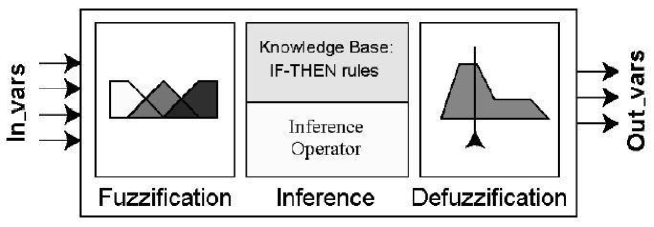
Figure 1: Basic structure of the fuzzy inference engine.

Like neural networks, the fuzzy logic systems are generic nonlinear function approximators [42]. In the realm of fuzzy logic this generic nonlinear function approximation is performed by means of fuzzy inference engine. The fuzzy inference engine is an input–output dynamical system which maps a set of input linguistic variables ($IF-$part) into a set of output linguistic variables ($THEN-$part). It has three sequential modules (see Figure 1):

1. Fuzzification; in this module numerical crisp input variables are fuzzified; this is performed as an overlapping partition of their universes of discourse by means of fuzzy membership functions $\mu(x)$ (1), which can have various shapes, like triangular, trapezoidal, Gaussian–bell,

   $$\mu(x)=\exp\left[\frac{-(x-m)^{2}}{2\sigma^{2}}\right],$$

   (with mean $m$ and standard deviation $\sigma$), sigmoid

   $$\mu(x)=\left[1+\left(\frac{x-m}{\sigma}\right)^{2}\right]^{-1},$$

   or some other shapes (see Figure 2).

   

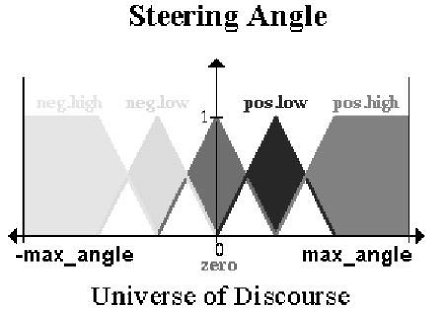
   Figure 2: Fuzzification example: set of triangular–trapezoidal membership functions partitioning the universe of discourse for the angle of the hypothetical steering wheel; notice the white overlapping triangles.

   B. Kosko and his students have done extensive computer simulations looking for the best shape of fuzzy sets to model a known test system as closely as possible. They let fuzzy sets of all shapes and sizes compete against each other. They also let neural systems tune the fuzzy–set curves to improve how well they model the test system. The main conclusion from these experiments is that ‘triangles never do well’ in such contests. Suppose we want an adaptive fuzzy system $F:\mathbb{R}^{n}\rightarrow\mathbb{R}$ to approximate a test function or approximand $f:\mathbb{R}^{n}\rightarrow\mathbb{R}$ as closely as possible in the sense of minimizing the mean–squared error between them, $\left(\left\|f-F\right\|^{2}\right)$. Then the $i$th scalar ‘sinc’ function (as commonly used in signal processing),

   $$\mu_{i}(x)=\frac{\sin\left(\frac{x-m_{i}}{d_{i}}\right)}{\frac{x-m_{i}}{d_{i}}},\qquad i=1,...,n,$$ (2)

   with center $m_{i}$ and dispersion (width) $d_{i}=\sigma_{i}^{2}>0$, often gives the best performance for $IF-$part mean–squared function approximation, even though this generalized function can take on negative values (see [48]).

2. Inference; this module has two submodules:

   (i) The expert–knowledge base consisting of a set of $IF-THEN$ rules relating input and output variables, and

   (ii) The inference method, or implication operator, that actually combines the rules to give the fuzzy output; the most common is Mamdani Min–Max inference, in which the membership functions for input variables are first combined inside the $IF-THEN$ rules using $AND$ ($\cap$, or $Min$) operator, and then the output fuzzy sets from different $IF-THEN$ rules are combined using $OR$ ($\cup$, or $Max$) operator to get the common fuzzy output (see Figure 3).

   

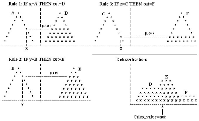
   Figure 3: Mamdani’s Min–Max inference method and Center of Gravity defuzzification.

3. Defuzzification; in this module fuzzy outputs from the inference module are converted to numerical crisp values; this is achieved by one of the several defuzzification algorithms; the most common is the Center of Gravity method, in which the crisp output value is calculated as the abscissa under the center of gravity of the output fuzzy set (see Figure 3).

In more complex technical applications of general function approximation (like in complex control systems, signal and image processing, etc.), two optional blocks are usually added to the fuzzy inference engine [42, 49, 50]:

0. Preprocessor, preceding the fuzzification module, performing various kinds of normalization, scaling, filtering, averaging, differentiation or integration of input data; and

4. Postprocessor, succeeding the defuzzification module, performing the analog operations on output data.

Common fuzzy systems have a simple feedforward mathematical structure, the so–called Standard Additive Model (SAM, for short), which aids the spread of applications. Almost all applied fuzzy systems use some form of SAM, and some SAMs in turn resemble the ANN models (see [48]).

In particular, an additive fuzzy system $F:\mathbb{R}^{n}\rightarrow\mathbb{R}^{p}$ stores $m$ rules of the patch form $A_{i}\times B_{i}\subset\mathbb{R}^{n}\times\mathbb{R}^{p}$, or of the word form ‘If $X=A_{i}$ Then $Y=B_{i}$’ and adds the ‘fired’ Then–parts $B_{i}^{{}^{\prime}}(x)$ to give the output set $B(x)$, calculated as

$$B(x)=\sum_{i=1}^{n}w_{i}B_{i}^{{}^{\prime}}(x)=\sum_{i=1}^{n}w_{i}\mu_{i}(x)B_{i}(x),\qquad i=1,...,n,$$ (3)

for a scalar rule weight $w_{i}>0$. The factored form $B_{i}^{{}^{\prime}}(x)=\mu_{i}(x)B_{i}(x)$ makes the additive system (3) a SAM system. The fuzzy system $F$ computes its output $F(x)$ by taking the centroid of the output set $B(x)$: $F(x)=$ Centroid$(B(x))$. The SAM Theorem then gives the centroid as a simple ratio,

$$F(x)=\sum_{i=1}^{n}p_{i}(x)c_{i},\qquad i=1,...,n,$$

where the convex coefficients or discrete probability weights $p_{i}(x)$ depend on the input $x$ through the ratios

$$p_{i}(x)=\frac{w_{i}\mu_{i}(x)V_{i}}{\sum_{k=1}^{n}w_{k}\mu_{k}(x)V_{k}},\qquad i=1,...,n.$$ (4)

$V_{i}$ is the finite positive volume (or area if $p=1$ in the codomain space $\mathbb{R}^{p}$) [48],

$$V_{i}=\int_{\mathbb{R}^{p}}b_{i}(y_{1},...,y_{p})dy_{1}...dy_{p}>0,$$

and $c_{i}$ is the centroid of the Then–part set $B_{i}(x)$,

$$c_{i}=\frac{\int_{\mathbb{R}^{p}}y\,b_{i}(y_{1},...,y_{p})dy_{1}...dy_{p}}{\int_{\mathbb{R}^{p}}b_{i}(y_{1},...,y_{p})dy_{1}...dy_{p}}.$$

2.2 Fuzzy Decision Making

Recall that finite state machines (FSMs) are simple ‘machines’ that have a finite number of states (or conditions) and transition functions that determine how input to the system changes it from one state to another [38].

Fuzzy State Machines (FuSMs) are a modification of FSMs. In FuSMs, the inputs to the system (that cause the transitions between states) are not discrete. The real value of FuSMs comes from the interaction of the system inputs. For example, a character in a video game may of a simple combat scenario decides how aggressive he will be depending on his health, the enemy’s health, and his distance from the enemy. The combination of these inputs cause the state transitions to happen. This can result in very complex behaviors from a small set of rules. For example,

The health variables have three sets:  Near death, Good, and Excellent.

The distance variable has three sets:  Close, Medium, and Far.

Finally, the output (aggressiveness) has three sets:  Run away, Fight defensively, and All out attack!.

Fuzzy Control Language (FCL) is a standard for Fuzzy Control Programming published by the International Electrotechnical Commission (IEC).

Fuzzy–logic decision maker (FLDM) breaks the decision scenario down into small parts that we can focus on and input easily. It then uses theoretically optimal methods of combining the scenario pieces into a global interrelated whole with an indication as to which alternative is the best within the constraints and goals of the decision scenario.

The assumption in FLDM is that a judgment consists of a known here and now (the constraints), a hoped for future there and then (the goals), and various paths (the alternatives) for getting from the present here and now to the future there and then. The problem is then the selection of the path (alternative) that optimally supports the present constraints and the future goals.

Decision making when faced with several alternatives, which initially appear equally good or desirable, can be a time consuming and often painful process. The FLDM overcomes the (human) memory and processor limitations by allowing the decision maker to selectively evaluate small amounts of the necessary information at any one time (i.e., the fuzzy values of goal and constraint satisfaction and simple, one-at-a-time paired comparisons). Then, when it becomes necessary to evaluate all the pertinent data, the computer can be utilized to perform the decision task in a straight forward manner.

2.3 Fuzzy Logic Control

The most common and straightforward applications of fuzzy logic are in the domain of control [42, 49, 50, 51]. Fuzzy control is a nonlinear control method based on fuzzy logic. Just as fuzzy logic can be described simply as computing with words rather than numbers, fuzzy control can be described simply as control with sentences rather than differential equations.

A fuzzy controller is based on the fuzzy inference engine, which acts either in the feedforward or in the feedback path, or as a supervisor for the conventional PID controller.

A fuzzy controller can work either directly with fuzzified dynamical variables, like direction, angle, speed, or with their fuzzified errors and rates of change of errors. In the second case we have rules of the form:

1. If error is $Neg$ and change in error is $Neg$ then output is $NB$.

2. If error is $Neg$ and change in error is $Zero$ then output is $NM$.

The collection of rules is called a rule base. The rules are in $IF-THEN$ format, and formally the $IF-$side is called the condition and the $THEN-$side is called the conclusion (more often, perhaps, the pair is called antecedent - consequent). The input value $Neg$ is a linguistic term short for the word Negative, the output value $NB$ stands for $Negative\_Big$ and $NM$ for $Negative\_Medium$. The computer is able to execute the rules and compute a control signal depending on the measured inputs error and change in error.

The rulebase can be also presented in a convenient form of one or several rule matrices, the so–called $FAM-$matrices, where $FAM$ is a shortcut for Kosko’s fuzzy associative memory [42, 49] (see Figure 4). For example, a $9\times 9$ graded FAM matrix can be defined in a symmetrical weighted form:

$$\text{FAM}=\left(\begin{tabular}[]{ccccc}0.6S4&0.6S4&0.7S3&...&CE\\ 0.6S4&0.7S3&0.7S3&...&0.9B1\\ 0.7S3&0.7S3&0.8S2&...&0.9B1\\ ...&...&...&...&0.6B4\\ CE&0.9B1&0.9B1&...&0.6B4\end{tabular}\ \ \right),$$

in which the vector of nine linguistic variables $L^{9}$ partitioning the universes of discourse of all three variables (with trapezoidal or Gaussian bell–shaped membership functions) has the form

$$L^{9}=\{S4,S3,S2,S1,CE,B1,B2,B3,B4\}^{T},$$

to be interpreted as: ‘small 4’, … , ‘small 1’, ‘center’, ‘big 1’, … , ‘big 4’. For example, the left upper entry $(1,1)$ of the FAM matrix means: IF red is S4 and blue is S4, THEN result is 0.6S4; or, entry $(3,7)$ means: IF red is S2 and blue is B2, THEN result is center, etc.

Here we give design examples for three fuzzy controllers.

Temperature Control System.

In this simple example, the input linguistic variable is

$temperature\_error=desired\_temperature-current\_temperature$. The two output linguistic variables are: $hot\_fan\_speed$, and $cool\_fan\_speed$. The universes of discourse, consisting of membership functions, i.e., overlapping triangular–trapezoidal shaped intervals, for all three variables are:

$invar$: $temperature\_error=\{Negative\_Big,Negative\_Medium,\newline Negative\_Small,Zero,Positive\_Small,Positive\_Medium,Positive\_Big\}$, with the range $[-110,110]$ degrees;

$outvars$: $hot\_fan\_speed$ and $cool\_fan\_speed=\{zero,low,medium,high,\newline very\_high\}$, with the range $[0,100]$ rounds-per-meter.

Car Anti–Lock Braking System.

The fuzzy—logic controller for the car anti–lock braking system consists of the following input variables:

slip_r (rear_wheels_slip),

slip_fr (front_right_wheel_slip),

slip_fl (front_left_wheel_slip),

with their membership functions:

NZ = Near_Zero,   OP = Optimal,   AO = Above_Optimal,

and the following output variables:

bp_r (rear_wheels_brake_pressure),

bp_fr (front_right_brake_pressure),

bp_fl (front_left_brake_pressure),

with their membership functions:

LW = Low,   MD = Medium,   HG = High.

The inference rule–base for this example consists of the following fuzzy implications:

IF  slip_fl is NZ  THEN  bp_fl is MD;

IF  slip_fr is NZ  THEN  bp_fr is MD;

IF  slip_r is NZ  THEN  bp_r is MD;

IF  slip_fl is OP  THEN  bp_fl is HG;

IF  slip_fr is OP  THEN  bp_fr is HG;

IF  slip_r is OP  THEN  bp_r is HG;

IF  slip_fl is AO  THEN  bp_fl is LW;

IF  slip_fr is AO  THEN  bp_fr is LW;

IF  slip_r is AO  THEN  bp_r is LW.

Truck Backer–Upper Steering Control System.

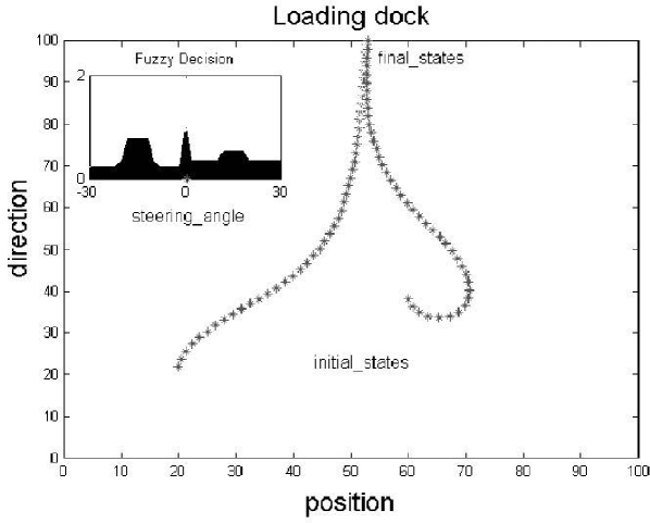
Figure 4: Truck backer–upper steering control system.

In this example there are two input linguistic variables: position and direction of the truck, and one output linguistic variable: steering angle (see Figure 4). The universes of discourse, partitioned by overlapping triangular–trapezoidal shaped intervals, are defined as:

$invars$: $position=\{NL,NS,ZR,PS,PL\}$,   and

$direction=\{NL,NM,NS,ZR,PS,PM,PL\}$, where $NL$ denotes Negative_Large, $NM$ is Negative_Medium, $NS$ is Negative_Small, etc.

$outvar$: $steering\_angle=\{NL,NM,NS,ZR,PS,PM,PL\}$.

The rule–base is given as:

IF direction is $NL$ and position is $NL$, THEN steering angle is $NL$;

IF direction is $NL$ and position is $NS$, THEN steering angle is $NL$;

IF direction is $NL$ and position is $ZR$, THEN steering angle is $PL$;

IF direction is $NL$ and position is $PS$, THEN steering angle is $PL$;

IF direction is $NL$ and position is $PL$, THEN steering angle is $PL$;

IF direction is $NM$ and position is $NL$, THEN steering angle is $ZR$;

. . . . . . . . . . . . .

IF direction is $PL$ and position is $PL$, THEN steering angle is $PL$.

The so–called control surface for the truck backer–upper steering control system is depicted in Figure 5.

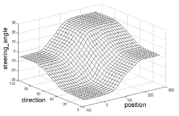
Figure 5: Control surface for the truck backer–upper steering control system.

2.3.1 Characteristics of Fixed Fuzzy Control

Fuzzy logic offers several unique features that make it a particularly good choice for many control problems, among them [50, 51]:

1. It is inherently robust since it does not require precise, noise–free inputs and can be programmed to fail safely if a feedback sensor quits or is destroyed. The output control is a smooth control function despite a wide range of input variations.

2. Since the fuzzy logic controller processes user–defined rules governing the target control system, it can be modified and tweaked easily to improve or drastically alter system performance. New sensors can easily be incorporated into the system simply by generating appropriate governing rules.

3. Fuzzy logic is not limited to a few feedback inputs and one or two control outputs, nor is it necessary to measure or compute rate–of–change parameters in order for it to be implemented. Any sensor data that provides some indication of a systems actions and reactions is sufficient. This allows the sensors to be inexpensive and imprecise thus keeping the overall system cost and complexity low.

4. Because of the rule-based operation, any reasonable number of inputs can be processed (1–8 or more) and numerous outputs (1–4 or more) generated, although defining the rulebase quickly becomes complex if too many inputs and outputs are chosen for a single implementation since rules defining their interrelations must also be defined. It would be better to break the control system into smaller chunks and use several smaller fuzzy logic controllers distributed on the system, each with more limited responsibilities.

5. Fuzzy logic can control nonlinear systems that would be difficult or impossible to model mathematically. This opens doors for control systems that would normally be deemed unfeasible for automation.

A fuzzy logic controller is usually designed using the following steps:

1. Define the control objectives and criteria: What am I trying to control? What do I have to do to control the system? What kind of response do I need? What are the possible (probable) system failure modes?

2. Determine the input and output relationships and choose a minimum number of variables for input to the fuzzy logic engine (typically error and rate–of–change of error).

3. Using the rule–based structure of fuzzy logic, break the control problem down into a series of IF X AND Y THEN Z rules that define the desired system output response for given system input conditions. The number and complexity of rules depends on the number of input parameters that are to be processed and the number fuzzy variables associated with each parameter. If possible, use at least one variable and its time derivative. Although it is possible to use a single, instantaneous error parameter without knowing its rate of change, this cripples the systems ability to minimize overshoot for a step inputs.

4. Create fuzzy logic membership functions that define the meaning (values) of Input/Output terms used in the rules.

5. Test the system, evaluate the results, tune the rules and membership functions, and re-test until satisfactory results are obtained.

Therefore, fuzzy logic does not require precise inputs, is inherently robust, and can process any reasonable number of inputs but system complexity increases rapidly with more inputs and outputs. Distributed processors would probably be easier to implement. Simple, plain–language rules of the form IF X AND Y THEN Z are used to describe the desired system response in terms of linguistic variables rather than mathematical formulas. The number of these is dependent on the number of inputs, outputs, and the designers control response goals. Obviously, for very complex systems, the rule–base can be enormous and this is actually the only drawback in applying fuzzy logic.

2.3.2 Pro and Contra Fuzzy Logic Control

According to [52] there are the following pro and contra arguments regarding fuzzy logic control:

1. Fuzzy logic control is more useful than its detractors claim.

2. Fuzzy logic control is less useful than its proponents claim.

3. Fuzzy logic does not generate a control law. It maps an existing control law from one set of rules into a logic set.

4. Fuzzy logic control is most useful in ‘common sense’ control situations, i.e., ones where it might be difficult to write down the equations of motion, but a human would know how to control it. Examples of this are the ‘truck backer upper’, car parking, train control, and helicopter control problems.

5. Fuzzy logic sets effectively quantize their input and output space. However, the quantization intervals are rarely uniform.

6. In most fuzzy logic control success stories the sample rates are incredibly high relative to the dynamics of the system. Much of their success is because of this.

Most of the examples of fuzzy logic control being successfully applied fall into the category of things that humans do well [52, 53, 54].

Recall that in Japan, there is a train (Sendai subway), which is controlled by fuzzy logic. The train pulls into the station within a few inches of its target. More accurate, but nevertheless replacing human control [53].

Also in Japan, there are experiments in controlling a small model helicopter (Spectrum, July 1992) via radio control. The helicopter can respond to commands such as take off and land, hover, forward, backwards, left and right [52, 53, 54].

Proponents assert that a conventional control scheme would be incredibly hard to design because it would be really tough to model the helicopter dynamics. The ‘model free’ nature of fuzzy logic control makes the problem trivial. This might be true, at least from a practical application point of view, but it obscures some key facts [52]:

1. The model helicopter was designed so that a human operator with a joystick could control it, i.e., it was designed to respond well to intuitive control rules. Because of this, the helicopter has been designed to be very robust to imprecision. (Robustness to imprecision is one of the features that many proponents claim fuzzy logic brings to the problem. It is possible that this feature is more a feature of the dynamic system than of fuzzy logic itself. In fact, L. Zadeh, the creator of fuzzy logic, points out that fuzzy logic takes advantage of a system’s inherent robustness to imprecision rather than creating a robustness to imprecision).

2. The human operator has an implicit model in his mind of the input-output behavior of the helicopter. This is how he generates his control law for using the joystick.

3. Fuzzy logic maps the human’s control law and therefore is based on the human’s implicit model of the helicopter. This in turn works because the helicopter was designed to be robust to human control actions.

4. The human being’s ‘bandwidth’ is quite low, certainly less than 100 Hz. Furthermore, it is unlikely that a toy helicopter, a train, or a truck would respond to anything about 1 Hz and certainly not 10 Hz. (Since it must be an issue in every digital control problem and since any implementation of fuzzy logic control involves using some digital processor, the natural conclusion is that the sample rates are chosen so high above the system time constants that they seemingly stop being important.)

The train control problem, as well as the car parking and truck backer upper problem are all described by (1-4) above. So we can conclude that high sample rates are an inherent part of using fuzzy logic. The seemingly unimportant high sample rate may be precisely why the simple control rules work well. Fast sampling does lead to a greater computational burden. However, the computational cost many be offset by being able to use a simpler control law.

If we look in any fuzzy logic article we will see a picture of membership functions for fuzzy sets (see, e.g., [53]). These sets effectively quantize the interval that they are on: they span the space so that any value on the line must fall into at least one of the sets. However, they do not behave quite like what we think of as quantizers since a particular value can be a member of more than one set. The sets are typically fairly coarse in terms of what we would consider effective quantization. Combinations of these coarse quantizers provide various fuzzy conditions. The coarse quantizations and simple rules may offset the higher sample rate requirement.

In summary, fuzzy logic does not generate a control law, it merely maps a law from one form to another. The simple rules for train control or truck backing up are not generated by fuzzy logic control. These are already present in the mind of the human operator. Fuzzy logic merely maps the intuitive rules into a computer program.

What seems to be the newest feature of fuzzy logic control is that because the borders are fuzzy, more than one logic state can be true to some degree. This allows for a smooth transition between one control action and another, since they can both go on but at different activation levels, or gain. Quite often control systems have different operating regimes. Handling the transitions between these tends to be ad hoc. Things, which are already ad hoc, are perfect candidates for using fuzzy logic. Thus, fuzzy logic might be a good solution for smoothly switching a control system from one operating regime to another. In the transition, both control laws would be active, but their outputs would be scaled by the how much the system is in one regime or another. Clearly, this means that both control laws would have to be run in parallel during the transition.

On the other hand, quite a lot has been said about the model–free nature of a fuzzy logic control system. The notion is that rather than trying to construct these complicated dynamic models for a system, the ‘simple fuzzy rules’ allow the designer to design a control system. Clearly, this hides the notion that buried in those ‘simple fuzzy rules’ is an implicit model of the system. Following [52], we believe that no intelligent action is possible without a model. Any general behavior trend constitutes a model, whether explicit (e.g. dynamic systems model) or implicit (i.e. as encompassed in the fuzzy logic rules).

Another general idea that seems to permeate the fuzzy logic control hype is the notion that someone with very little skill can design a controller using fuzzy logic, while using classical control takes years of training.

In fact, the advantages and disadvantage of fuzzy systems result of the fact that fuzzy logic represents a decision making process. In control field, this provides a wide range of viable ways to solve naturally control problems while the basic control knowledge is not needed [56].

Another thing to point out is that usually the fuzzy logic rules use more external sensors, including acceleration, velocity, and the position information. So they naturally perform better than conventional controllers (position feedback loop) based only on position sensors.

Many proponents of fuzzy logic control argue that fuzzy logic works much better than conventional control when the system is nonlinear. However, the conventional controller they are comparing it to is a PID controller based on a linear system model.

In the sense that the fuzzy logic rules encompass a better model (implicit but there) of the system than an inappropriately applied linear model, the fuzzy logic rules will work better. Recall that the linear model has its faults as well. If a control system is designed using a linear model that doesn’t characterize the system behavior well, then the control system will probably fail to work well. However, a fair comparison would be one made between a fuzzy logic controller and a nonlinear state feedback controller that measures all the same variables at the same sampling rate as the fuzzy logic controller. If such a comparison is made there is no guarantee that the fuzzy logic controller will work better.

3 Adaptive Fuzzy Control in Human Operator Modeling

3.1 Neuro–Fuzzy Hybrid Systems

In many applications, desired system behavior is partially represented by data sets. In control systems, these data sets may represent operational states. In decision support systems and data analysis applications, these data sets may represent sample cases.

Discussing the respective strengths and weaknesses of fuzzy logic and neural net technology, a simple comparison indicates that the strongest benefit of a neural net is that it can automatically learn from sample data. However, a neural net remains a black box, thus manual modification and verification of a trained net is not possible in a direct way.

This is where fuzzy logic excels: In a fuzzy logic system, any component is defined as close as possible to human intuition, making it very easy to manually modify and verify a designed system. However, fuzzy logic systems can not automatically learn from sample data.

This is where neuro–fuzzy system provides ‘the best of both worlds’. Take the explicit representation of knowledge in linguistic variables and rules from fuzzy logic and add the learning approach used with neural nets. In the neuro–fuzzy system, both fuzzy rules and membership functions are adjusted by some form of backpropagation learning to adapt the system behavior according to the sample data.

The neuro–fuzzy system can also be used to optimize existing fuzzy logic systems. Starting with an existing fuzzy logic system, the neuro–fuzzy system interactively tunes rule weights and membership function definitions so that the system converges to the behavior represented by the data sets.

To distinguish between more and less important rules in the knowledge base, we can put weights on them. Such weighted knowledge base can be then trained by means of artificial neural networks. In this way we get hybrid neuro–fuzzy trainable expert systems.

Another way of the hybrid neuro–fuzzy design is the fuzzy inference engine such that each module is performed by a layer of hidden artificial neurons, and ANN–learning capability is provided to enhance the system knowledge (see Figure 6).

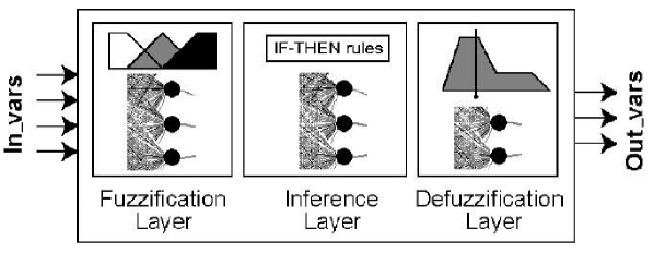
Figure 6: Neuro–fuzzy inference engine.

Again, the fuzzy control of the backpropagation learning can be implemented as a set of heuristics in the form of fuzzy $IF-THEN$ rules, for the purpose of achieving a faster rate of convergence. The heuristics are driven by the behavior of the instantaneous sum of squared errors.

As another alternative, we can consider the well–known fuzzy ARTMAP system, which is essentially a clustering algorithm (vector quantizer), with supervision that redirects training inputs which would be grouped in an incorrect category to a different cluster. A fuzzy ARTMAP system consists of two fuzzy ART modules, each of which clusters vectors in an unsupervised fashion, linked by a map field. Fuzzy ART clusters vectors based on two separate distance criteria, match and choice. For more details, see [57].

Finally, most feedback fuzzy systems are either discrete or continuous generalized SAMs [48], given respectively by

$$x(k+1)=\sum_{i=1}^{n}p_{i}(x(k))B_{i}(x(k)),\qquad\text{or}\qquad\dot{x}(t)=\sum_{i=1}^{n}p_{i}(x(t))B_{i}(x(t)),$$

with coefficients $p_{i}$ given by (4) above.

3.2 Neuro–Fuzzy–Fractal Operator Control

Although the general concept of learning, according to the schematic recursion

$$NEW\,\,VALUE_{t_{n+1}}\,=\,OLD\,\,VALUE_{t_{n}}\,+\,INNOVATION$$

– can be implemented in the framework of nonlinear control theory (as seen in the previous subsection), its natural framework is artificial intelligence.

For the purpose of neuro–fuzzy–fractal control [38, 39], the general model for a nonlinear plant can be modified as [35, 36]

$$\dot{x} = f_{1}(x,D,\alpha)-\beta f_{2}(x,D,\alpha),$$ (5)

$$\dot{y} = \beta f_{2}(x,D,\alpha),$$

where $x\in\mathbb{R}^{n}$ is a vector of state variables, $y\in\mathbb{R}^{m}$ is a vector of the system outputs, $\beta\in\mathbb{R}$ is a constant measuring the efficiency of the conversion process, $D\in(0,3)$ is the fractal dimension of the process, and $\alpha\in\mathbb{R}$ is a fuzzy–inference selection parameter.

For a complex dynamical system it may be necessary to consider a set of mathematical models to represent adequately all of possible dynamic behaviors of the system. In this case, we need a decision scheme to select the appropriate model to use according to the linguistic value of a selection parameter. We use a fuzzy inference system for differential equations to achieve the model selection. We have fuzzy rules of the form:

IF $\alpha$ is $A_{1}$ AND $D$ is $B_{1}$ THEN $M_{1}$

…      …      …

IF $\alpha$ is $A_{n}$ AND $D$ is $B_{n}$ THEN $M_{n}$

where $A_{1},...,A_{n}$ are linguistic values for $\alpha,B_{1},...,B_{n}$ are linguistic values for the fractal dimension $D$, and $M_{1},...,M_{n}$ are mathematical models of the form given by 5. The selection parameter $\alpha$ represents the environment variable, like temperature, humidity, etc.

Following [35, 36], we combine adaptive model–based control using neural networks with the method for model selection using fuzzy logic and fractal theory, to obtain a hybrid neuro–fuzzy–fractal method for control of nonlinear plants. This general method combines the advantages of neural networks (ability for identification and control) with the advantages of fuzzy logic (ability for decision and use of expert knowledge) to achieve the goal of robust adaptive control of nonlinear dynamic plants. We also use the fractal dimension to characterize the plant–output processes in modeling these dynamical systems.

3.2.1 Fractal Dimension for Machine Output Identification

The experimental identification of a nonlinear biologic transducer is often approached via consideration of its response to a stochastic test ensemble, such as Gaussian white noise [44]. In this approach, the input–output relationship a deterministic transducer is described by an orthogonal series of functionals. Laboratory implementation of such procedures requires the use of a particular test signal drawn from the idealized stochastic ensemble; the statistics of the particular test signal necessarily deviate from the statistics of the ensemble. The notion of a fractal dimension (specifically the capacity dimension) is a means to characterize a complex time series. It characterizes one aspect of the difference between a specific example of a test signal and the test ensemble from which it is drawn: the fractal dimension of ideal Gaussian white noise is infinite, while the fractal dimension of a particular test signal is finite. The fractal dimension of a test signal is a key descriptor of its departure from ideality: the fractal dimension of the test signal bounds the number of terms that can reliably be identified in the orthogonal functional series of an unknown transducer [45].

Definition of the fractal dimension.

Recall that for a smooth (i.e., nonfractal) line, an approximate length $L(r)$ is given by the minimum number $N$ of segments of length $r$ needed to cover the line, $L(r)=Nr$. As $r$ goes to zero, $L(r)$ approaches a finite limit, the length $L$ of the curve. Similarly one can define the area $A$ or the volume $V$ of nonfractal objects as the limit of an integer power law of $r$,

$$A=\lim_{r\rightarrow 0}Nr,\text{ \ \ \ \ \ \ \ \ }V=\lim_{r\rightarrow 0}Nr^{3},$$

where the integer exponent is the Euclidean dimension $E$ of the object.

This definition can not be used for fractal objects: as $r$ tends to $0$, we enter finer and finer details of the fractal and the product $Nr^{E}$ may diverge to infinity. However, a real number $D$ exists so that the limit of $Nr^{D}$ stays finite. This exponent is called Hausdorff dimension $D_{H}$, defined by

$$D_{H}=\lim_{r\rightarrow 0}\frac{\log N}{\log(1/r)}.$$

Another popular definition of dimension proposed for fractal objects is the correlation dimension $D_{2}$, given by

$$D_{2}=\lim_{r\rightarrow 0}\frac{\log C(r)}{\log(r)},$$

where $C(r)$ is the number of points which have a smaller (Euclidean) distance than a given distance $r$. This measure is widely used because it is easy to evaluate for experimental data, when the fractal comes from a ‘dust’ of isolated points. A method for measuring $D_{2}$ of strange attractors can be found in [47]. $D_{2}$ may also be used to determine whether a time–series derives from a random process or from a deterministic chaotic system. $m-$dimensional data vectors are constructed from $m$ measurements spaced equidistant in time, and $D_{2}$ is evaluated for this $m-$dimensional set of points. If the time–series is a random process, $D_{2}$ increases with $m$; if the time–series is a deterministic signal, $D_{2}$ does not increase further when the embedding dimension m exceeds $D_{2}$. Thus a plot of the correlation dimension as a function of the embedding dimension may easily show whether a signal is random noise of deterministic chaos. Note that $D_{2}\leq D_{H}.$

Fractal behavior and singularities in time series.

The functions $y(t)$ typically studied in mathematical analysis are continuous and have continuous derivatives. Hence, they can be approximated in the vicinity of some time $t_{i}$ by Taylor series (or power series)

$$y(t)=a_{0}+a_{1}(t-t_{i})+a_{2}(t-t_{i})^{2}+a_{3}(t-t_{i})^{3}+...$$ (6)

For small regions around $t_{i}$, just a few terms of the expansion (6) are necessary to approximate the function $y(t)$. In contrast, most time series $y(t)$ found in ‘real–life’ applications appear quite noisy). Therefore, at almost every point in time, they cannot be approximated either by Taylor series (or by Fourier series) of just a few terms. Moreover, many experimental or empirical time series have fractal features, i.e., for some times $t_{i}$, the series $y(t)$ displays singular behavior [46, 46]. By this, we mean that at those times ti, the signal has components with non–integer powers of time which appear as step-like or cusp-like features, the so–called singularities, in the signal.

Formally, one can write

$$y(t)=a_{0}+a_{1}(t-t_{i})+a_{2}(t-t_{i})^{2}+a_{3}(t-t_{i})^{3}+...+a_{h}(t-t_{i})^{h_{i}}$$ (7)

where $t$ is inside a small vicinity of $t_{i}$, and $h_{i}$ is a non–integer number quantifying the local singularity of $y(t)$ at $t=t_{i}$.

The next problem is to quantify the ‘frequency’ in the signal of a particular value $h$ of the singularity exponents $h_{i}$. Different possibilities can be considered. For example, the set of times with singular behavior {$t_{i}$} may be a finite fraction of the time series and homogeneously distributed over the signal. But {$t_{i}$} may also be an asymptotically infinitesimal fraction of the entire signal and have a very heterogeneous structure. That is, the set {$t_{i}$} may be a fractal itself. In either case, it is useful to quantify the properties of the sets of singularities in the signal by calculating their fractal dimensions $D_{2}$ or $D_{H}$.

Fractal dimension of a machine output signal.

This method uses the fractal dimension to make a unique classification of the different types of machine behavior, because different types of signals have different geometrical forms. The problem is then of finding a one–to–one map between the different types of machine behaviors and their corresponding fractal dimension. The first step in obtaining this map is to find experimentally the different geometrical forms for machine output signals. The second step is to calculate the corresponding fractal dimensions for these signals. This fractal dimension can be calculated for a selected type of signals with several samples, to obtain as a result a statistical estimation of the fractal dimension and the corresponding error of the estimation. In order to make an efficient use of this map between the different types of machine behaviors and their corresponding estimated dimensions, we need to implement it as a module in the computer program.

3.2.2 Fuzzy Logic Model Selection for Dynamical Systems

For a real–world dynamical system it may be necessary to consider a set of mathematical models to represent adequately all of the possible dynamic behaviors of the system. In this case, we need a fuzzy decision procedure to select the appropriate model to use according to the value of a selection parameter vector $\alpha$. To implement this decision procedure, we need a fuzzy inference system that can use differential equations as consequents. For this purpose, we can follow the fuzzy decision system developed in [35, 36], that can be considered as a generalization of the classical Sugeno’s inference system [40, 41, 42], in which differential equations as consequents of the fuzzy rules are used instead of simple polynomials like in the original Sugeno’s method. Using this method, a fuzzy model for a general dynamical system can be expressed as follows [38]:

IF $\alpha_{1}$ is $A_{11}$ AND $\alpha_{2}$ is $A_{12}$ … AND $\alpha_{m}$ is $A_{1m}$ THEN $\dot{y}=f_{1}(y,\alpha)$

IF $\alpha_{1}$ is $A_{21}$ AND $\alpha_{2}$ is $A_{22}$ … AND $\alpha_{m}$ is $A_{2m}$ THEN $\dot{y}=f_{2}(y,\alpha)$

…      …      …

IF $\alpha_{1}$ is $A_{n1}$ AND $\alpha_{2}$ is $A_{n2}$ … AND $\alpha_{m}$ is $A_{nm}$ THEN $\dot{y}=f_{n}(y,\alpha)$

where $A_{ij}$ is the linguistic value of $\alpha_{j}$ for the $i$th rule, $\alpha=[\alpha_{1},...,\alpha_{m}]\in\mathbb{R}^{m}$, and $y\in\mathbb{R}^{p}$ is the output obtained by the numerical solution of the corresponding differential equation (it is assumed that each differential equation in this fuzzy model locally approximates the real dynamical system over a neighborhood (or region) of $\mathbb{R}^{m}$).

For example, if a complex dynamical system is modelled by using four different mathematical models $(M_{1},M_{2},M_{3},M_{4})$ of the form (5), the decision scheme can be expressed as a single–input fuzzy model [35, 36]

IF $\alpha$ is small THEN $\dot{y}=f_{1}(y,\alpha)$,

IF $\alpha$ is regular THEN $\dot{y}=f_{2}(y,\alpha)$,

IF $\alpha$ is medium THEN $\dot{y}=f_{3}(y,\alpha)$,

IF $\alpha$ is large THEN $\dot{y}=f_{4}(y,\alpha)$.

where the output $y$ is obtained by the numerical solution of the corresponding differential equation.

3.2.3 Parametric Adaptive Control Using Neural Networks

A feedforward neural network model takes an input vector $X$ and produces an output vector $Y$. The input–output map $NN:X\rightarrow Y$ is determined by the network architecture (see, e.g., [42, 43]). The feedforward network generally consists of at least three layers: one input layer, one output layer, and one or more hidden layers. In our case, the input layer with $y+1$ processing elements, i.e., one for each predictor variable plus a processing element for the bias. The bias element always has an input of one, $X_{y+1}=1$. Each processing element in the input layer sends signals $X_{i}\,(i=1,...,y+1)$ to each of the $q$ processing elements in the hidden layer. The $q$ processing elements in the hidden layer (indexed by $j=1,...,q$) produce an ‘activation’ $a_{j}=F\left(\sum w_{ij}X_{i}\right)$ where $w_{ij}$ are the weights associated with the connections between the $y+1$ processing elements of the input layer and the $j$th processing element of the hidden layer. Once again, processing element $q+1$ of the hidden layer is a bias element and always has an activation of one, i.e. $a_{q+1}=1$. Assuming that the processing element in the output layer is linear, the network model will be

$$Y_{t}=\sum_{l=1}^{p+1}\pi_{l}x_{it}+\sum_{j=1}^{p+1}\theta_{j}F\left(\sum_{j=1}^{p+1}w_{ij}X_{it}\right).$$ (8)

Here $\pi_{l}$ are the weights for the connections between the input layer and the output layer, and $\theta_{j}$ are the weights for the connections between the hidden layer and the output layer. The main requirement to be satisfied by the activation function $F(\cdot)$ is that it be nonlinear and differentiable. Typical functions used are the sigmoid, $F(x)=1/(1+\exp(-x))$ and hyperbolic tangent, $F(x)=(\exp(x)-\exp(-x))/(\exp(x)+\exp(-x))$.

Feedforward neural nets are trained by supervised training, the most popular being some form of the backpropagation algorithm. As the name suggests, the error computed from the output layer is backpropagated through the network, and the weights are modified according to their contribution to the error function. Essentially, backpropagation performs a local gradient search, and hence its implementation does not guarantee reaching a global minimum. A number of heuristics are available to partly address this problem, for practical purpose the best one is the Levenberg–Marquardt algorithm. Instead of distinguishing between the weights of the different layers as in (8), we refer to them generically as $w_{ij}$ in the following. After some mathematical simplification the weight change $\Delta w_{ij}$ equation suggested by backpropagation can be expressed as (see, e.g., [43, 42])

$$\Delta w_{ij}=-\eta(\partial E_{1}/\partial w_{ij})+\theta\Delta w_{ij},$$ (9)

where $\eta$ is the learning coefficient and $\theta$ is the momentum term. One heuristic that is used to prevent the neural network from getting stuck at a local minimum is the random presentation of the training data. Another heuristic that can speed up convergence is the cumulative update of weights, i.e., weights are not updated after the presentation of each input–output pair, but are accumulated until a certain number of presentations are made, this number referred to as an ‘epoch’. In the absence of the second term in (9), setting a low learning coefficient results in slow learning, whereas a high learning coefficient can produce divergent behavior. The second term in (9) reinforces general trends, whereas oscillatory behavior is cancelled out, thus allowing a low learning coefficient but faster learning. Last, it is suggested that starting the training with a large learning coefficient and letting its value decay as training progresses speeds up convergence.

Now, parametric adaptive control is the problem of controlling the output of a system with a known structure but unknown parameters. These parameters can be considered as the elements of a vector $y$. If $y$ is known, the parameter vector of a controller can be chosen as $\theta^{\ast}$ so that the plant together with the fixed controller behaves like a reference model described by a difference (or differential) equation with constant coefficients [37]. If $y$ is unknown, the vector $\theta(t)$ has to be adjusted on–line using all the available information concerning the system.

Two distinct approaches to the adaptive control of an unknown plant are (i) direct control and (ii) indirect control. In direct control, the parameters of the controller are directly adjusted to reduce some norm of the output error. In indirect control, the parameters of the plant are estimated as $y(t)$ at any time instant and the parameter vector $\theta(t)$ of the controller is chosen assuming that $y(t)$ represents the true value of the plant parameter vector. Even when the plant is assumed to be linear and time–invariant, both direct and indirect adaptive control results in non–linear systems.

When indirect control is used to control a nonlinear system, the plant is parameterized using a mathematical model of the general form (5) and the parameters of the model are updated using the identification error. The controller’s parameters in turn are adjusted by backpropagating the error (between the identified model and the reference model outputs) through the identified model.

4 Application: Fuzzy-Control Based Tennis Simulator

In this section we present a fuzzy–logic model for the tennis game, consisting of two stages: attack (AT) and counter–attack (CA). For technical details, see [38].

4.0.1 Attack Model: Tennis Serve

A. Simple Attack: Serve Only. The simple AT–dynamics is represented by a single fuzzy associative memory (FAM) map

$$\underset{CAT}{TARGET}\quad\underset{FAM}{{\makebox[42.00003pt]{\rule[-1.49994pt]{0.0pt}{18.74664pt}\raisebox{1.50009pt}{\begin{picture}(4.2,0.4)(-0.3,-0.2)\put(1.8,0.2){\makebox(0.0,0.0)[b]{${\cal F}^{AT}$}}\put(0.0,0.0){\vector(1,0){3.6}}\end{picture}}}}}\quad\underset{CAT}{ATTACK}$$

In the case of simple tennis serve, this AT–scenario reads

$$\underset{OPPONENT-IN}{O\ni o_{m}}\quad{\makebox[42.00003pt]{\rule[-1.49994pt]{0.0pt}{18.74664pt}\raisebox{1.50009pt}{\begin{picture}(4.2,0.4)(-0.3,-0.2)\put(1.8,0.2){\makebox(0.0,0.0)[b]{${\cal F}^{AT}$}}\put(0.0,0.0){\vector(1,0){3.6}}\end{picture}}}}\quad\underset{SERVE-OUT}{SR\ni sr_{n}}$$

where the two $n-$categories, $O_{\dim=2}\ni o_{m}$ and $SR_{\dim=3}\ni sr_{n}$, contain the temporal fuzzy variables $\{o_{m}=o_{m}(t)\}$ and $\{sr_{n}=sr_{n}(t)\}$, respectively opponent–related (target information) and serve–related, partitioned by overlapping Gaussians, $\mu(z)=\\ exp\left[\frac{-(z-m)^{2}}{2\sigma^{2}}\right]$, and defined as:

$\underset{OPPONENT-IN}{O}:\begin{array}[]{l}o_{1}=Opp.Posit.Left.Right:(center,medium,wide),\\ o_{2}=Opp.Antcp.Lft.Rght:(runCenter,stay,runWide),\\ \end{array}$

$\underset{SERVE-OUT}{SR}:\begin{array}[]{l}sr_{1}=1.Serve.Speed:(low,medium,high)\\ sr_{2}=2.Serve.Spin:(low,medium,high)\\ sr_{3}=3.Serve.Placement:(center,medium,wide)\end{array}$

In the fuzzy–matrix form this simple serve reads

$$\overset{O:\,OPPONENT-IN}{\left[\begin{array}[]{l}o_{1}=Opp.Posit.Left.Right\\ o_{2}=Opp.Anticip.Left.Right\end{array}\right]}\quad{\makebox[37.80003pt]{\rule[-1.34995pt]{0.0pt}{16.87198pt}\raisebox{1.35008pt}{\begin{picture}(4.2,0.4)(-0.3,-0.2)\put(1.8,0.2){\makebox(0.0,0.0)[b]{${\cal F}^{AT}$}}\put(0.0,0.0){\vector(1,0){3.6}}\end{picture}}}}\quad\overset{SR:\;SERVE-OUT}{\left[\begin{array}[]{l}sr_{1}=1.Serve.Speed\\ sr_{2}=2.Serve.Spin\\ sr_{3}=3.Serve.Place\end{array}\right]}$$

B. Attack–Maneuver: Serve–Volley. The generic advanced AT–dynamics is given by a composition of FAM functors

$$\underset{CAT}{TARGET}\quad\underset{FAM}{{\makebox[42.00003pt]{\rule[-1.49994pt]{0.0pt}{18.74664pt}\raisebox{1.50009pt}{\begin{picture}(4.2,0.4)(-0.3,-0.2)\put(1.8,0.2){\makebox(0.0,0.0)[b]{${\cal F}^{AT}$}}\put(0.0,0.0){\vector(1,0){3.6}}\end{picture}}}}}\quad\underset{CAT}{ATTACK}\quad\underset{FAM}{{\makebox[42.00003pt]{\rule[-1.49994pt]{0.0pt}{18.74664pt}\raisebox{1.50009pt}{\begin{picture}(4.2,0.4)(-0.3,-0.2)\put(1.8,0.2){\makebox(0.0,0.0)[b]{${\cal G}^{AT}$}}\put(0.0,0.0){\vector(1,0){3.6}}\end{picture}}}}}\quad\underset{CAT}{MANEUVER}$$

In the case of advanced tennis serve, this AT–scenario reads

$$\underset{OPPONENT-IN}{O\ni o_{m}}{\makebox[42.00003pt]{\rule[-1.49994pt]{0.0pt}{18.74664pt}\raisebox{1.50009pt}{\begin{picture}(4.2,0.4)(-0.3,-0.2)\put(1.8,0.2){\makebox(0.0,0.0)[b]{${\cal F}^{AT}$}}\put(0.0,0.0){\vector(1,0){3.6}}\end{picture}}}}\underset{SERVE-OUT}{SR\ni sr_{n}}{{\makebox[42.00003pt]{\rule[-1.49994pt]{0.0pt}{18.74664pt}\raisebox{1.50009pt}{\begin{picture}(4.2,0.4)(-0.3,-0.2)\put(1.8,0.2){\makebox(0.0,0.0)[b]{${\cal G}^{AT}$}}\put(0.0,0.0){\vector(1,0){3.6}}\end{picture}}}}}\quad\underset{RUN-VOLEY}{RV\ni rv_{p}}$$

where the new $n-$category, $RV_{\dim=2}\ni rv_{p}$, contains the opponent–anticipation driven volley–maneuver, expressed by fuzzy variables $\{rv_{p}=rv_{p}(t)\}$, partitioned by overlapping Gaussians and given by:

$\underset{RUN-VOLEY}{RV}:\begin{array}[]{l}rv_{1}=RV.For:(baseLine,center,netClose)\\ rv_{2}=RV.L.R.:(left,center,right)\end{array}$

In the fuzzy–matrix form this advanced serve reads

$$\overset{O:\,OPPONENT-IN}{\left[\begin{array}[]{l}o_{1}=Opp.Posit.L.R.\\ o_{2}=Opp.Anticip.L.R.\end{array}\right]}{\makebox[37.80003pt]{\rule[-1.34995pt]{0.0pt}{16.87198pt}\raisebox{1.35008pt}{\begin{picture}(4.2,0.4)(-0.3,-0.2)\put(1.8,0.2){\makebox(0.0,0.0)[b]{${\cal F}^{AT}$}}\put(0.0,0.0){\vector(1,0){3.6}}\end{picture}}}}\overset{SR:\;SERVE-OUT}{\left[\begin{array}[]{l}sr_{1}=1.Serve.Speed\\ sr_{2}=2.Serve.Spin\\ sr_{3}=3.Serve.Place\end{array}\right]}{\makebox[37.80003pt]{\rule[-1.34995pt]{0.0pt}{16.87198pt}\raisebox{1.35008pt}{\begin{picture}(4.2,0.4)(-0.3,-0.2)\put(1.8,0.2){\makebox(0.0,0.0)[b]{${\cal G}^{AT}$}}\put(0.0,0.0){\vector(1,0){3.6}}\end{picture}}}}\overset{RV:\;RUN-VOLEY}{\left[\begin{array}[]{l}rv_{1}=RV.For\\ rv_{2}=RV.L.R\end{array}\right]}$$

4.0.2 Counter–Attack Model: Tennis Return

A. Simple Return. The simple CA–dynamics reads:

$$\underset{CAT}{ATTACK}\quad\underset{FAM}{{\makebox[42.00003pt]{\rule[-1.49994pt]{0.0pt}{18.74664pt}\raisebox{1.50009pt}{\begin{picture}(4.2,0.4)(-0.3,-0.2)\put(1.8,0.2){\makebox(0.0,0.0)[b]{${\cal F}^{CA}$}}\put(0.0,0.0){\vector(1,0){3.6}}\end{picture}}}}}\quad\underset{CAT}{MANEUVER}\quad\underset{FAM}{{\makebox[42.00003pt]{\rule[-1.49994pt]{0.0pt}{18.74664pt}\raisebox{1.50009pt}{\begin{picture}(4.2,0.4)(-0.3,-0.2)\put(1.8,0.2){\makebox(0.0,0.0)[b]{${\cal G}^{CA}$}}\put(0.0,0.0){\vector(1,0){3.6}}\end{picture}}}}}\quad\underset{CAT}{RESPONSE}$$

In the case of simple tennis return, this CA–scenario consists purely of conditioned–reflex reaction, no decision process is involved, so it reads:

$$\underset{BALL-IN}{B\ni b_{{\cal K}}}\quad{{\makebox[42.00003pt]{\rule[-1.49994pt]{0.0pt}{18.74664pt}\raisebox{1.50009pt}{\begin{picture}(4.2,0.4)(-0.3,-0.2)\put(1.8,0.2){\makebox(0.0,0.0)[b]{${\cal F}^{CA}$}}\put(0.0,0.0){\vector(1,0){3.6}}\end{picture}}}}}\quad\underset{RUNNING}{R\ni r_{{\cal J}}}\quad{{\makebox[42.00003pt]{\rule[-1.49994pt]{0.0pt}{18.74664pt}\raisebox{1.50009pt}{\begin{picture}(4.2,0.4)(-0.3,-0.2)\put(1.8,0.2){\makebox(0.0,0.0)[b]{${\cal G}^{CA}$}}\put(0.0,0.0){\vector(1,0){3.6}}\end{picture}}}}}\quad\underset{SHOT-OUT}{S\ni s_{k}}$$

where the $n-$categories $B_{\dim=5}\ni b_{{\cal K}},$ $R_{\dim=3}\ni r_{{\cal J}},$ $S_{\dim=4}\ni s_{k}$, contain the fuzzy variables $\{b_{{\cal K}}=b_{{\cal K}}(t)\},$ $\{r_{{\cal J}}=r_{{\cal J}}(t)\}$ and $\{s_{k}=s_{k}(t)\}$, respectively defining the ball inputs, our player’s running maneuver and his shot–response, K.e.,

$$\overset{B:\;BALL-IN}{\left[\begin{array}[]{l}b_{1}=Dist.L.R.\\ b_{2}=Dist.{\cal F}.B.\\ b_{3}=Dist.Vert\\ b_{4}=Speed\\ b_{5}=Spin\end{array}\right]}{{\makebox[37.80003pt]{\rule[-1.34995pt]{0.0pt}{16.87198pt}\raisebox{1.35008pt}{\begin{picture}(4.2,0.4)(-0.3,-0.2)\put(1.8,0.2){\makebox(0.0,0.0)[b]{${\cal F}^{CA}$}}\put(0.0,0.0){\vector(1,0){3.6}}\end{picture}}}}}\overset{R:\;RUNNING}{\left[\begin{array}[]{l}r_{1}=Run.L.R.\\ r_{2}=Run.{\cal F}.B.\\ r_{3}=Run.Vert\end{array}\right]}{{\makebox[37.80003pt]{\rule[-1.34995pt]{0.0pt}{16.87198pt}\raisebox{1.35008pt}{\begin{picture}(4.2,0.4)(-0.3,-0.2)\put(1.8,0.2){\makebox(0.0,0.0)[b]{${\cal G}^{CA}$}}\put(0.0,0.0){\vector(1,0){3.6}}\end{picture}}}}}\overset{S:\;SHOT-OUT}{\left[\begin{array}[]{l}s_{1}=Backhand\\ s_{2}=Forehand\\ s_{3}=Voley\\ s_{4}=Smash\end{array}\right]}$$

Here, the existence of efficient weapons within the $\underset{SHOT-OUT}{S}$ arsenal–space, namely $s_{k}(t):s_{1}=Backhand,s_{2}=Forehand,s_{3}=Voley$ and $s_{4}=Smash$, is assumed.

The universes of discourse for the fuzzy variables $\{b_{{\cal K}}(t)\},$ $\{r_{{\cal J}}(t)\}$ and $\{s_{k}(t)\}$, partitioned by overlapping Gaussians, are defined respectively as:

$\underset{BALL-IN}{B}:\begin{array}[]{l}b_{1}=Dist.L.R.:(veryLeft,left,center,right,veryRight),\\ b_{2}=Dist.{\cal F}.B.:(baseLine,center,netClose),\\ b_{3}=Dist.Vert:(low,medium,high),\\ b_{4}=Speed:(low,medium,high),\\ b_{5}=Spin:(highTopSpin,lowTopSpin,flat,\\ \qquad\qquad\qquad lowBackSpin,highBackSpin).\end{array}$

$\underset{RUNNING}{R}:\\ \begin{array}[]{l}r_{1}=Run.L.R.:(veryLeft,left,center,right,veryRight),\\ r_{2}=Run.{\cal F}.B.:(closeFront,front,center,back,farBack),\\ r_{3}=Run.Vert:(squat,normal,jump).\end{array}$

$\underset{SHOT-OUT}{S}:\begin{array}[]{l}s_{1}=Backhand:(low,medium,high),\\ s_{2}=Forehand:(low,medium,high),\\ s_{3}=Voley:(backhand,block,forehand),\\ s_{4}=Smash:(low,medium,high).\end{array}$

B. Advanced Return. The advanced CA–dynamics includes both the information about the opponent and (either conscious or subconscious) decision making. This generic CA–scenario is formulated as the following composition + fusion of FAM functors:

$$\underset{CAT}{ATTACK}\underset{FAM}{{\makebox[42.00003pt]{\rule[-1.49994pt]{0.0pt}{18.74664pt}\raisebox{1.50009pt}{\begin{picture}(4.2,0.4)(-0.3,-0.2)\put(1.8,0.2){\makebox(0.0,0.0)[b]{${\cal F}^{CA}$}}\put(0.0,0.0){\vector(1,0){3.6}}\end{picture}}}}}\underset{CAT}{MANEUV}\underset{FAM}{{\makebox[42.00003pt]{\rule[-1.49994pt]{0.0pt}{18.74664pt}\raisebox{1.50009pt}{\begin{picture}(4.2,0.4)(-0.3,-0.2)\put(1.8,0.2){\makebox(0.0,0.0)[b]{${\cal G}^{CA}$}}\put(0.0,0.0){\vector(1,0){3.6}}\end{picture}}}}}\;\underset{CAT}{DECISION}\underset{FAM}{{\makebox[42.00003pt]{\rule[-1.49994pt]{0.0pt}{18.74664pt}\raisebox{1.50009pt}{\begin{picture}(4.2,0.4)(-0.3,-0.2)\put(1.8,0.2){\makebox(0.0,0.0)[b]{${\cal H}^{CA}$}}\put(0.0,0.0){\vector(1,0){3.6}}\end{picture}}}}}\;\;\underset{CAT}{RESP}{{{}{}{}{}\put(-1100.0,-550.0){\makebox(0.0,0.0)[]{$\vphantom{}$}}{{}{}{}{}\put(-1090.0,-550.0){\makebox(0.0,0.0)[]{$\vphantom{}$}}}{}{}{}{}{}\put(-1095.0,-570.0){\makebox(0.0,0.0)[]{$$}}}{{}{}{}{}\put(-1100.0,-50.0){\makebox(0.0,0.0)[]{$\vphantom{}$}}{{}{}{}{}\put(-1090.0,-50.0){\makebox(0.0,0.0)[]{$\vphantom{}$}}}{}{}{}{}{}\put(-1095.0,-30.0){\makebox(0.0,0.0)[]{$$}}}{{}{}{}{}\put(-1100.0,-50.0){\makebox(0.0,0.0)[]{$$}}{{}{}{}{}\put(-1100.0,-550.0){\makebox(0.0,0.0)[]{$$}}}{{\put(-1100.0,-480.0){\vector(0,1){360.0}}}}{}{}{}{}\put(-1140.0,-300.0){\makebox(0.0,0.0)[r]{${\cal K}^{CA}$}}}{{}{}{}{}\put(-1090.0,-50.0){\makebox(0.0,0.0)[]{$$}}{{}{}{}{}\put(-1090.0,-550.0){\makebox(0.0,0.0)[]{$$}}}{{}}{}{}{}{}\put(-1050.0,-300.0){\makebox(0.0,0.0)[l]{$FAM$}}}}\put(-1280.0,-600.0){$\underset{CAT}{TARGET}$}$$

where we have added two new $n-$categories, $\underset{CAT}{TARGET}$ and $\underset{CAT}{DECISION}$, respectively containing information about the opponent as a target, as well as our own aiming decision processes. In the case of advanced tennis return, this reads:

$$\underset{BALL-IN}{B\ni b_{{\cal K}}}\;\;{{\makebox[42.00003pt]{\rule[-1.49994pt]{0.0pt}{18.74664pt}\raisebox{1.50009pt}{\begin{picture}(4.2,0.4)(-0.3,-0.2)\put(1.8,0.2){\makebox(0.0,0.0)[b]{${\cal F}^{CA}$}}\put(0.0,0.0){\vector(1,0){3.6}}\end{picture}}}}}\;\;\underset{RUNNING}{R\ni r_{{\cal J}}}\;\;{{\makebox[42.00003pt]{\rule[-1.49994pt]{0.0pt}{18.74664pt}\raisebox{1.50009pt}{\begin{picture}(4.2,0.4)(-0.3,-0.2)\put(1.8,0.2){\makebox(0.0,0.0)[b]{${\cal G}^{CA}$}}\put(0.0,0.0){\vector(1,0){3.6}}\end{picture}}}}}\;\;\underset{DECISION}{D\ni d_{l}}\;\;{{\makebox[42.00003pt]{\rule[-1.49994pt]{0.0pt}{18.74664pt}\raisebox{1.50009pt}{\begin{picture}(4.2,0.4)(-0.3,-0.2)\put(1.8,0.2){\makebox(0.0,0.0)[b]{${\cal H}^{CA}$}}\put(0.0,0.0){\vector(1,0){3.6}}\end{picture}}}}}\;\;\underset{SHOT-OUT}{S\ni s_{k}}{{{}{}{}{}\put(-1200.0,-550.0){\makebox(0.0,0.0)[]{$\vphantom{}$}}{{}{}{}{}\put(-1190.0,-550.0){\makebox(0.0,0.0)[]{$\vphantom{}$}}}{}{}{}{}{}\put(-1195.0,-570.0){\makebox(0.0,0.0)[]{$$}}}{{}{}{}{}\put(-1200.0,-50.0){\makebox(0.0,0.0)[]{$\vphantom{}$}}{{}{}{}{}\put(-1190.0,-50.0){\makebox(0.0,0.0)[]{$\vphantom{}$}}}{}{}{}{}{}\put(-1195.0,-30.0){\makebox(0.0,0.0)[]{$$}}}{{}{}{}{}\put(-1200.0,-50.0){\makebox(0.0,0.0)[]{$$}}{{}{}{}{}\put(-1200.0,-550.0){\makebox(0.0,0.0)[]{$$}}}{{\put(-1200.0,-480.0){\vector(0,1){360.0}}}}{}{}{}{}\put(-1240.0,-300.0){\makebox(0.0,0.0)[r]{${\cal K}^{CA}$}}}{{}{}{}{}\put(-1190.0,-50.0){\makebox(0.0,0.0)[]{$$}}{{}{}{}{}\put(-1190.0,-550.0){\makebox(0.0,0.0)[]{$$}}}{{}}}}\put(-1500.0,-580.0){$\underset{OPPONENT-IN}{O\ni o_{m}}$}$$

where the two additional $n-$categories, $O_{\dim=4}\ni o_{m}$ and $D_{\dim=5}\ni d_{l}$, contain the fuzzy variables $\{o_{m}=o_{m}(t)\}$ and $\{d_{l}=d_{l}(t)\}$, respectively defining the opponent–related target information and the aim–related decision processes, both partitioned by overlapping Gaussians and defined as:

$\underset{OPPONENT-IN}{O}:\begin{array}[]{l}o_{1}=Opp.Posit.L.R.:(left,center,right),\\ o_{2}=Opp.Posit.{\cal F}.B.:(netClose,center,baseLine),\\ o_{3}=Opp.Anticip.L.R.:(runLeft,stay,runRight),\\ o_{4}=Opp.Anticip.{\cal F}.B.:(runNet,stay,runBase).\end{array}$

$\underset{DECISION}{D}:\begin{array}[]{l}d_{1}=Aim.L.R.:(left,center,right),\\ d_{2}=Aim.{\cal F}.B.:(netClose,center,baseLine),\\ d_{3}=Aim.Vert:(low,medium,high),\\ d_{4}=Aim.Speed:(low,medium,high),\\ d_{5}=Aim.Spin:(highTopSpin,lowTopSpin,noSpin,\\ \qquad\qquad\qquad\qquad lowBackSpin,highBackSpin).\end{array}$

The corresponding fuzzy–matrices read:

$$\overset{B:\;BALL-IN}{\left[\begin{array}[]{l}b_{1}=Dist.L.R.\\ b_{2}=Dist.{\cal F}.B.\\ b_{3}=Dist.Vert\\ b_{4}=Speed\\ b_{5}=Spin\end{array}\right]},\qquad\overset{R:\;RUNNING}{\left[\begin{array}[]{l}r_{1}=Run.L.R.\\ r_{2}=Run.{\cal F}.B.\\ r_{3}=Run.Vert\end{array}\right]},\qquad\overset{D:\;DECISION}{\left[\begin{array}[]{l}d_{1}=Aim.L.R.\\ d_{2}=Aim.{\cal F}.B.\\ d_{3}=Aim.Vert\\ d_{4}=Aim.Speed\\ d_{5}=Aim.Spin\end{array}\right]},$$

$${\left[\overset{O:\,OPPONENT-IN}{\begin{array}[]{l}o_{1}=Opp.Posit.L.R.\\ o_{2}=Opp.Posit.{\cal F}.B.\\ o_{3}=Opp.Anticip.L.R.\\ o_{4}=Opp.Anticip.{\cal F}.B.\end{array}}\right]},\qquad\overset{S:\;SHOT-OUT}{\left[\begin{array}[]{l}s_{1}=Backhand\\ s_{2}=Forehand\\ s_{3}=Voley\\ s_{4}=Smash\end{array}\right].}$$

5 Conclusion

In this paper we have presented several control strategies for human operator and sport modelling. Roughly, they are deviled into fixed-fuzzy control methods and adaptive-fuzzy control methods. As an application of the presented fuzzy control approaches to sport modelling we have presented a fuzzy-control based tennis simulator, consisting of attack and counter-attack stages. This approach can be applied to all sport games.

References

- [1] Wickens, C.D., The Effects of Control Dynamics on Performance, in Handbook of Perception and Human Performance, Vol II, Cognitive Process and Performance (Ed. Boff, K.R., Kaufman, L., Thomas, J.P.), Wiley, New York, (1986).
- [2] Wiener, N., Cybernetics, New York, (1961).
- [3] Doherty, G., Continuous Interaction and Manual Control, ERCIM News 40, January, (2000).
- [4] Ivancevic, V., Ivancevic, T., Geometrical Dynamics of Complex Systems. Springer, Dordrecht, (2006).
- [5] Phillips, J.M., Anderson, M.R., A Variable Strategy Pilot Model, 2000 AIAA Atmospheric Flight Mechanics Conference, Denver, Colorado, August, (2000).
- [6] Phillips, J.M., Variable Strategy Model of the Human Operator, PhD thesis in Aerospace Engineering, Blacksburg, VI, (2000).
- [7] McRuer, D.T., Jex, H.R., A Review of Quasi-Linear Pilot Models, IEEE Transactions on Human Factors in Electronics, Vol. HFE-8, 3, 231-249, (1967).
- [8] McRuer, D.T., Krendel E.S., Mathematical Models of Human Pilot Behavior, North Atlantic Treaty Organization Advisory Group for Aerospace Research and Development, AGARD-AG-188, January, (1974).
- [9] Kleinman, D.L., Baron, S., Levinson, W.H., An Optimal Control Model of Human Response, Part I: Theory and Validation, Automatica, 6(3), 357-369, (1970).
- [10] Sheridan, T.B., Ferrell, W., Man-Machine Systems: Information, Control, and Decision Models of Human Performance, MIT Press: Cambridge, MA, (1974).
- [11] Innocenti, M., Belluchi, A., Balestrion, A., New Results on Human Operator Modelling During Non-Linear Behavior in the Control Loop, 1997 American Control Conference, Albuquerque, NM, June 4-6 1997, Vol. 4, American Automatic Control Council, Evanston, IL, 2567-2570, (1997).
- [12] Innocenti, M., Petretti, A., Vellutini, M., Human Operator Modelling During Discontinuous Performance, 1998 AIAA Atmospheric Flight Mechanics Conference, Boston, Massachusetts, 31-38, August, (1998).
- [13] McRuer, D., Allen, W., Weir, D., The Man/Machine Control Interface - Precognitive and Pursuit Control, Proc. Joint Automatic Control Conference, Vol. II, 81-88, Philadelphia, Pennsylvania, October, (1978).
- [14] Young, L.R., Meiry, J.L., Bang-Bang Aspects of Manual Control in High-Order Systems, IEEE Tr. Aut. Con. AC-10, 336-341, July, (1965).
- [15] Pew, R.W., Performance of Human Operators in a Three-State Relay Control System with Velocity-Augmented Displays, IEEE Tr. Human Factors, HFE-7(2), 77-83, (1966).
- [16] Diamantides, N.D., A Pilot Analog for Aircraft Pitch Control, J. Aeronaut. Sci. 25, 361-371, (1958).
- [17] Costello, R.G., The Surge model of theWell-Trained Human Operator in SimpleManual Control, IEEE Tr. Man-Mach. Sys. MMS-9(1), 2-9, (1968).
- [18] Hess, R.A., A Rational for Human Operator Pulsive Control Behavior, J. Guid. Con. Dyn. 2(3), 221-227, (1979).
- [19] Phatak, A.V., Bekey, G.A., Model of the Adaptive Behavior of the Human Operator in Response to a Sudden Change in the Control Situation, IEEE Tr. Man-Mach. Sys. MMS-10(3), 72-80, (1969).
- [20] Pitkin, E.T., A Non-Linear Feedback Model for Tracking Studies, Proceedings of the Eight Annual Conference on Manual Control, University ofMichigan, Ann Arbor, Michigan, 11-22, May, (1972).
- [21] Meritt, M.J., Bekey, G.A., An Asynchronous Pulse-Amplitude Pulse-Width Model of the Human Operator, Third Annual NASA-University Conf. Manual Control, 225-239, March, (1967).
- [22] Johannsen, G., Development and Optimization of a Nonlinear Multiparameter Human Operator Model, IEEE Tr. Sys. Man, Cyber. 2(4), 494-504, (1972).
- [23] Angel, E.S., Bekey, G.A., Adaptive Finite-State Models of Manual Control Systems, IEEE Tr. Man-Mach. Sys. 9(1), 15-20, (1968).
- [24] Costello, R., Higgins, R., An Inclusive Classified Bibliography Pertaining to Modeling the Human Operator as an Element in an Automatic Control System, IEEE Tr. Human Factors in Electronics, HFE-7(4), 174-181, (1966).
- [25] Andrisani, D., Gau, C.F., A Nonlinear Pilot Model for Hover, J. Guid. Con. Dyn. 8(3), 332-339, (1985).
- [26] Heffley, R., Pilot Models for Discrete Maneuvers, 1982 AIAA Guidance, Navigation, and Control Conference Proceedings, 132-142, San Diego, CA, August, (1982).
- [27] Hess, R.A., Structural Model of the Adaptive Human Pilot, J. Guid. Con. Dyn. 3(5), 416-423, (1980).
- [28] Moorehouse, D., Modelling a Distracted Pilot for Flying Qualities Applications, 1995 AIAA Atmospheric Flight Mechanics Conference, 14-24, Baltimore, Maryland, August, (1995).
- [29] Ivancevic, V., Ivancevic, T., Human-Like Biomechanics: A Unified Mathematical Approach to Human Biomechanics and Humanoid Robotics. Springer, Dordrecht, (2005)
- [30] Ivancevic, V., Ivancevic, T., Complex Dynamics: Advanced System Dynamics in Complex Variables. Springer, Dordrecht, (2007).
- [31] Ivancevic, T., Jain, L. Pattison, J., Hariz, A., Nonlinear Dynamics and Chaos Methods in Neurodynamics and Complex Data Analysis. Nonl. Dyn. (Springer Online First)
- [32] Ivancevic, V., Ivancevic, T., High–Dimensional Chaotic and Attractor Systems. Springer, Berlin, (2006).
- [33] Ivancevic, V., Ivancevic, T., Complex Nonlinearity: Chaos, Phase Transitions, Topology Change and Path Integrals, Springer, Series: Understanding Complex Systems, Berlin, (2008).
- [34] Ivancevic, T.T., Jovanovic, B., Djukic, S., Djukic, M., Markovic, S., Complex Sports Biodynamics: With Practical Applications in Tennis, Springer, Cognitive Systems Monographs, (2009).
- [35] Melin, P., Castillo, O., A New Method for Adaptive Model-Based Neuro-Fuzzy-Fractal Control of Non-Linear Dynamic Plants: The Case of Biochemical Reactors. Proceedings of IPMU ’98, 1, 475-482, EDK Publ. Paris, (1998).
- [36] Melin, P., Castillo, O., A new method for adaptive model-based control of dynamic industrial plants using neural networks, fuzzy logic and fractal theory, Systems Analysis Modelling Simulation, 43(1), 1-15, (2003).
- [37] Jang, J.-S.R., Sun, C.-T., Neuro-fuzzy and soft computing: a computational approach to learning and machine intelligence, Prentice-Hall, Inc., Upper Saddle River, NJ, (1996).
- [38] Ivancevic, V., Ivancevic, T., Neuro-Fuzzy Associative Machinery for Comprehensive Brain and Cognition Modelling. Springer, Berlin, (2007).
- [39] Ivancevic, V., Ivancevic, T., Computational Mind: A Complex Dynamics Perspective. Springer, Berlin, (2007).
- [40] Sugeno, M., Kang, G.T., Structure identification of fuzzy model. Fuzzy Sets and Systems, 28, 15–33, (1988).
- [41] Takagi, T., Sugeno, M., Fuzzy identification of systems and its applications to modelling and control. IEEE Transactions on Systems, Man and Cybernetics, 20(2), 116–132, (1985).
- [42] Kosko, B., Neural Networks and Fuzzy Systems, A Dynamical Systems Approach to Machine Intelligence. Prentice–Hall, New York, (1992).
- [43] Haykin, S., Neural Networks: A Comprehensive Foundation. Macmillan, (1994).
- [44] Marmarelis, P.Z., Marmarelis, V.Z., Analysis of Physiological Systems: The White Noise Approach, Plenum Press, (1978).
- [45] Victor, J.D., The fractal dimension of a test signal: implications for system identification procedures, Biol. Cyber. 57, 421-426 (1987).
- [46] Amaral, L.A.N., Goldberger, A.L., Ivanov, P.Ch. & Stanley H.E., Scale-independent measures and pathologic cardiac dynamics. Phys. Rev. Lett. 81, 2388-2391, (1998).
- [47] Grassberger, P., Procaccia, I., Measuring the strangeness of a strange attractor. Physica D, 9, 189-208, (1983).
- [48] Kosko, B., The Fuzzy Future: From Society and Science to Heaven in a Chip. Random House, Harmony, (1999).
- [49] Kosko, B., Fuzzy Engineering. Prentice Hall, New York, (1996).
- [50] Lee, C.C., Fuzzy Logic in Control Systems. IEEE Trans. on Systems, Man, and Cybernetics, SMC, 20(2), 404–435, (1990).
- [51] Dote, Y., Strefezza, M., and Suitno, A., Neuro–fuzzy robust controllers for drive systems. in Neural Networks Applications, ed. P.K. Simpson, IEEE Techn. Upd. Ser., New York, (1996).
- [52] Abramovitch, D., Some Crisp Thoughts on Fuzzy Logic, in the Proceedings of the 1994 American Controls Conference in Baltimore, MD, June, (1994).
- [53] Cox, E., Fuzzy fundamentals, IEEE Spectrum, 29, 58-61, October, (1992).
- [54] Schwartz, D.G., Klir, G.J., Fuzzy logic flowers in Japan, IEEE Spectrum, 29, 32-35, July, (1992).
- [55] Kosko, B., Isaka, S., Fuzzy Logic, Sci. Amer. 269, 76-81, July, (1993).
- [56] Vibet, C., Fuzzy logic versus traditional control, Fuzzy Sets and Systems, (1994).
- [57] Carpenter, G.A., Grossberg, S., Markuson, N., Reynolds, J.H., Rosen, D.B., Fuzzy ARTMAP: A neural network architecture for incremental supervised learning of analog multidimensional maps, IEEE Trans. on Neural Networks, 3(5), 698-713, (1992).