Compton scattering off elementary spin $\frac{3}{2}$ particles

Abstract

We calculate Compton scattering off an elementary spin $\frac{3}{2}$ particle in a recently proposed framework for the description of high spin fields based on the projection onto eigen-subspaces of the Casimir operators of the Poincaré group. We also calculate this process in the conventional Rarita-Schwinger formalism. Both formalisms yield the correct Thomson limit but the predictions for the angular distribution and total cross section differ beyond this point. We point out that the average squared amplitudes in the forward direction for Compton scattering off targets with spin $s=0,\frac{1}{2},1$ are energy-independent and have the common value $4e^{4}$. As a consequence, in the rest frame of the particle the differential cross section for Compton scattering in the forward direction is energy independent and coincides with the classical squared radius. We show that these properties are also satisfied by a spin $3/2$ target in the Poincaré projector formalism but not by the Rarita-Schwinger spin $3/2$ particle.

I Introduction

A long standing problem in particle physics is the proper description of high spin fields. The widely used Rarita-Schwinger (RS) formalism RS was shown to be inconsistent for interacting particles long ago JS , and lead to superluminical propagation of spin 3/2 waves in the presence of an external electromagnetic field VZ . Similar and related problems have been found in the presence of other interactions todos .

Recently, a new formalism for the description of high spin fields was put forward NKR (NKR formalism in the following), based on the projection onto eigensubspaces of the Casimir operators of the Poincaré group. In that work, it is shown that, under minimal coupling, the (parity conserving) electromagnetic structure of a spin 3/2 particle transforming in the $(1/2,1/2)\otimes[(1/2,0)\oplus(0,1/2)]$ representation of the Homogeneous Lorentz Group (HLG) depend on two free parameters denoted $g$ and $f$. The propagation of spin 3/2 waves was studied for the case $f=0$ and it is shown there that the value of the gyromagnetic factor $g$ is related to the causality of the propagation of spin 3/2 waves and causal propagation is obtained for $g=2$. This result relates the “natural” value of the gyromagnetic factor naturalg to causality for spin $3/2$.

The case of spin 1 particles in the $\left(1/2,1/2\right)$ representation space of the HLG was addressed in NRDK . In this case, the most general electromagnetic interaction of a spin 1 vector particle was also shown to depend on two parameters (denoted $g$ and $\xi$) which cannot be fixed from the Poincaré projection alone. These parameters determine the electromagnetic structure of the particle and were fixed imposing unitarity at high energies for Compton scattering. This procedure fixes the parameters to $g=2$ and $\xi=0$ predicting a gyromagnetic factor $g=2$, a related quadrupole electric moment $Q=-e(g-1)/m^{2}$ and vanishing odd-parity couplings as a consequence of $\xi=0$ . The obtained couplings coincide with the ones predicted for the $W$ boson in the Standard Model SM .

These results make worthy to study the analogous problems for spin 3/2 particles and this work is devoted to this purpose. The electromagnetic properties of spin $3/2$ particles has been addressed in a number of previous papers aiming to understand either the electromagnetic structure of hypothetical elementary particles or the electromagnetic properties of hadrons naturalg ; let .

In this work we study the electromagnetic structure of a spin $3/2$ particle in the NKR formalism and calculate Compton scattering both in the NKR and RS formalisms. We compare the predictions of these formalisms for the angular distribution and total cross section and notice that the average squared amplitude for Compton scattering off spin $0,1/2$ and $1$ particles in the forward direction is energy independent. This property is satisfied by spin $3/2$ particles in the NKR formalism but not in the Rarita-Schwinger one. This paper is organized as follows: in the next section we revisit the electromagnetic structure of a spin 3/2 particle under $U(1)_{em}$ gauge principle in the NKR formalism, extract the corresponding Feynman rules and prove that Ward identities are satisfied. In section III we calculate the amplitude for Compton scattering, show that it is gauge invariant and work out the predictions for the differential and total cross sections. In section IV we calculate this process in the conventional Rarita-Schwinger formalism. We discuss our results in section V and give a summary in section VI.

II Electromagnetic interactions of spin 3/2 particles in the NKR formalism

The NKR Lagrangian for spin 3/2 interacting particles with charge $-e$ has been discussed in NKR and we refer the reader to this work for the details. The most general free Lagrangian for a spin 3/2 particle arising from the Poincaré projectors is

$${\cal L}_{0}(a,b) = (\partial^{\mu}\overline{\psi}^{\alpha})\Gamma_{\alpha\beta\mu\nu}\partial^{\nu}\psi^{\beta}-m^{2}\overline{\psi}^{\alpha}\psi_{\alpha}+\frac{1}{a}(\partial^{\mu}\overline{\psi}_{\mu})(\partial^{\alpha}\psi_{\alpha})+\frac{m^{2}}{b}(\overline{\psi}^{\mu}\gamma_{\mu})(\gamma^{\alpha}\psi_{\alpha}).$$ (1)

Here, $a$, $b$ are free (“gauge”) parameters and the corresponding (“gauge fixing”) terms are associated to the constraints (see NKR for a discussion on this point). The most general tensor compatible with Poincaré projection and Lorentz covariance is

$$\Gamma_{\alpha\beta\mu\nu}=B_{\alpha\beta\mu\nu}-ig[M_{\mu\nu}]_{\alpha\beta}+\tilde{d}\gamma^{5}[M_{\mu\nu}]_{\alpha\beta}+\tilde{c}\epsilon_{\alpha\beta\mu\nu}+if\gamma^{5}\epsilon_{\alpha\beta\mu\nu},$$ (2)

with

$$B_{\alpha\beta\mu\nu}= \frac{1}{3}\left(-\gamma_{\beta}\gamma_{\nu}g_{\alpha\mu}-2g_{\beta\nu}g_{\alpha\mu}+\gamma_{\alpha}\gamma_{\mu}g_{\beta\nu}-\gamma_{\alpha}\gamma_{\beta}g_{\mu\nu}+3g_{\alpha\beta}g_{\mu\nu}\right),$$ (3)

$$[M_{\mu\nu}]_{\alpha\beta}= \frac{1}{2}\sigma_{\mu\nu}g_{\alpha\beta}+i\left(g_{\mu\alpha}g_{\nu\beta}-g_{\mu\beta}g_{\nu\alpha}\right).$$ (4)

Here $M_{\mu\nu}$ are the generators of the $(1/2,1/2)\otimes[(1/2,0)\oplus(0,1/2)]$ representation of the H.L.G. and $\sigma_{\mu\nu}=\frac{i}{2}[\gamma_{\mu},\gamma_{\nu}]$. We included the odd-parity terms $\tilde{c},\tilde{d}$ for the sake of completeness. This tensor coincides with the one in Eq.(141) of NKR when $f=0$ and $\tilde{c}=\tilde{d}=0$; it has been slightly rewritten for convenience in the calculations below.

The propagator is calculated as the inverse of the kinetic term. We obtain NKR

$$S(p,a,b)=\frac{\Delta(p,a,b)}{p^{2}-m^{2}+i\epsilon},$$ (5)

with:

$$\Delta(p,a,b) = -{\mathbf{P}}^{\left(\frac{3}{2}\right)}-\xi\left[\left(bp^{2}+a(1-b)m^{2}\right){\mathbf{P}}^{\left(\frac{1}{2}\right)}_{11}+a(3-b)m^{2}{\mathbf{P}}^{\left(\frac{1}{2}\right)}_{22}-\sqrt{3}am^{2}({\mathbf{P}}^{\left(\frac{1}{2}\right)}_{12}+{\mathbf{P}}^{\left(\frac{1}{2}\right)}_{21})\right],$$ (6)

$$\xi = \frac{b}{m^{2}}\frac{p^{2}-m^{2}}{(3-b)\left(bp^{2}-a(1-b)m^{2}\right)-3am^{2}}.$$ (7)

Here, ${\mathbf{P}}^{\left(\frac{3}{2}\right)}$ stands for the spin 3/2 projector and ${\mathbf{P}}^{\left(\frac{1}{2}\right)}_{ij}$ are the spin 1/2 projectors (for $i=j$) and “switch” operators (for $i\neq j$) in the $(1/2,1/2)\otimes[(1/2,0)\oplus(0,1/2)]$ representation space of the HLG.

Electromagnetic interactions are introduced in Eq. (1) using the $U(1)_{em}$ gauge principle which amounts to use the minimal coupling recipe $\partial^{\alpha}\rightarrow D^{\alpha}=\partial^{\alpha}-ieA^{\alpha}$. We obtain

$${\cal L}(a,b)={\cal L}_{0}(a,b)-ej_{\mu}(a)A^{\mu}+e^{2}(\overline{\psi}^{a}\Gamma_{\alpha\beta\mu\nu}\psi^{\beta}+\frac{1}{a}\overline{\psi}_{\mu}\psi_{\nu})A^{\mu}A^{\nu},$$ (8)

with

$$j_{\mu}(a)=i\overline{\psi}^{\alpha}\Gamma_{\alpha\beta\mu\nu}\partial^{\nu}\psi^{\beta}-i\partial^{\nu}\overline{\psi}^{\alpha}\Gamma_{\alpha\beta\nu\mu}\psi^{\beta}+\frac{1}{a}(\overline{\psi}_{\mu}i\partial\cdot\psi-i\partial\cdot\overline{\psi}\psi_{\mu}).$$ (9)

In momentum space, using $\psi_{\alpha}=u_{\alpha}(p)e^{-ip\cdot x}$ the transition current reads

$$j_{\mu} = \overline{u}^{\alpha}(p^{\prime})\left[\Gamma_{\alpha\beta\nu\mu}p^{\prime\nu}+\Gamma_{\alpha\beta\mu\nu}p^{\nu}+\frac{1}{a}(g_{\mu\beta}p^{\prime}_{\alpha}+g_{\mu\alpha}p_{\beta})\right]u^{\beta}(p),$$ (10)

$$\equiv \overline{u}^{\alpha}(p^{\prime})\mathcal{V}(p^{\prime},p,a)_{\alpha\beta\mu}u^{\beta}(p),$$

where the electromagnetic vertex ${\cal V}(p^{\prime},p,a)$ is defined by the latter relation. The Feynman rules derived from Eq. (8) are shown in Fig. (1).

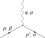
$$e\left[\Gamma_{\alpha\beta\nu\mu}p^{\prime\nu}+\Gamma_{\alpha\beta\mu\nu}p^{\nu}+\frac{1}{a}({g}_{\mu\alpha}p^{\beta}+{g}_{\mu\beta}p^{\prime\alpha})\right]$$

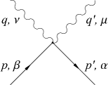
$$-\frac{1}{2}e^{2}\left[\Gamma_{\alpha\beta\mu\nu}+\Gamma_{\alpha\beta\nu\mu}+\frac{1}{a}({g}_{\alpha\mu}{g}_{\beta\nu}+{g}_{\beta\mu}{g}_{\alpha\nu})\right]$$

$$S_{\alpha\beta}(p,a,b)=\frac{\Delta_{\alpha\beta}(p,a,b)}{p^{2}-m^{2}+i\epsilon}$$

Figure 1: Feynman rules for arbitrary values of the “gauge” parameters $a,b$.

A straightforward calculation shows that this vertex satisfy

$$(p^{\prime}-p)^{\mu}{\cal V} (p^{\prime},p,a)_{\alpha\beta\mu}=$$

$$\left\{K_{\alpha\beta}(p^{\prime})+\frac{1}{a}(p^{\prime}_{\alpha}p^{\prime}_{\beta})-m^{2}{g}_{\alpha\beta}+\frac{m^{2}}{b}\gamma_{\alpha}\gamma_{\beta}\right\}-\left\{K_{\alpha\beta}(p)+\frac{1}{a}(p_{\beta}p_{\alpha})-m^{2}{g}_{\alpha\beta}+\frac{m^{2}}{b}\gamma_{\alpha}\gamma_{\beta}\right\},$$ (11)

where $K_{\alpha\beta}(p)\equiv\Gamma_{\alpha\beta\mu\nu}p^{\mu}p^{\nu}$. In terms of the inverse propagator we get

$$(p^{\prime}-p)^{\mu}{\cal V}(p^{\prime},p,a)_{\alpha\beta\mu}=S^{-1}_{\alpha\beta}(p^{\prime},a,b)-S^{-1}_{\alpha\beta}(p,a,b),$$ (12)

i.e. the Ward-Takahashi identity is satisfied for any value of $a,b$.

The calculations below simplify in the “unitary gauge” $a=b=\infty$, thus in the following we will work in this “gauge”. In this case

$$j_{\mu}=\overline{u}^{\alpha}(p^{\prime})(\Gamma_{\alpha\beta\nu\mu}p^{\prime\nu}+\Gamma_{\alpha\beta\mu\nu}p^{\nu})u^{\beta}(p)\equiv\overline{u}^{\alpha}(p^{\prime}){\cal O}(p^{\prime},p)_{\alpha\beta\mu}u^{\beta}(p),$$ (13)

and the electromagnetic vertex reads

$${\cal V}(p^{\prime},p,\infty)_{\alpha\beta\mu} \equiv {\cal O}(p^{\prime},p)_{\alpha\beta\mu}=\Gamma_{\alpha\beta\nu\mu}p^{\prime\nu}+\Gamma_{\alpha\beta\mu\nu}p^{\nu},$$ (14)

$$\overline{\mathcal{O}}(p^{\prime},p)_{\alpha\beta\mu} \equiv \gamma^{0}[{\mathcal{O}}(p^{\prime},p)_{\alpha\beta\mu}]^{\dagger}\gamma^{0}={\mathcal{O}}(p,p^{\prime})_{\beta\alpha\mu}.$$ (15)

The propagator in this case is

$$S(p,\infty,\infty)\equiv\Pi(p)=\frac{-\mathbf{P^{(\frac{3}{2})}}+\frac{p^{2}-m^{2}}{m^{2}}\mathbf{P}^{(\frac{1}{2})}}{p^{2}-m^{2}+i\epsilon}\equiv\frac{\Delta(p)}{p^{2}-m^{2}+i\epsilon},$$ (16)

and the Ward-Takahashi identity simplifies to

$$(p^{\prime}-p)^{\mu}\mathcal{O}(p^{\prime},p)_{\alpha\beta\mu}=\{K_{\alpha\beta}(p^{\prime})-m^{2}g_{\alpha\beta}\}-\{K_{\alpha\beta}(p)-m^{2}g_{\alpha\beta}\}=\Pi^{-1}_{\alpha\beta}(p^{\prime})-\Pi^{-1}_{\alpha\beta}(p).$$ (17)

III Compton Scattering

In this section we calculate Compton scattering. Our conventions are given in Fig (2).

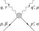
Figure 2: Compton scattering off a spin 3/2 particle.

We will work in the rest frame of the initial spin 3/2 particle (lab frame). In this frame the differential cross section reads

$$\frac{\textup{d}\sigma}{\textup{d}\Omega}=\frac{1}{4(4\pi)^{2}}\frac{|\overline{\mathcal{M}}|^{2}}{m^{2}}\left(\frac{\omega^{\prime}}{\omega}\right)^{2},$$ (18)

where $m$ stands for the mass of the spin 3/2 particle and $\omega$, $\omega^{\prime}$ denote the energies of the incoming and outgoing photon respectively. They are related by

$$\omega^{\prime}=\frac{m\omega}{m+\omega(1-\cos\theta)},$$ (19)

where $\theta$ stands for the angle of the outgoing photon with respect to the incoming one.

The amplitude for Compton scattering has three contributions:

$$\mathcal{M}=\mathcal{M}_{A}+\mathcal{M}_{B}+\mathcal{M}_{C}$$ (20)

where $\mathcal{M}_{A},$ $\mathcal{M}_{B}$ and $\mathcal{M}_{C}$ correspond to $s$-channel, $u$-channel exchange and the “seagull” contact term respectively:

$$\mathcal{M}_{A}= e^{2}\overline{u}^{\alpha}(p^{\prime})\mathcal{O}(p^{\prime},Q)_{\alpha\gamma\mu}\Pi^{\gamma\delta}(Q)\mathcal{O}(Q,p)_{\delta\beta\nu}u^{\beta}(p)\epsilon^{\mu*}(q^{\prime})\epsilon^{\nu}(q),$$ (21)

$$\mathcal{M}_{B}= e^{2}\overline{u}^{\alpha}(p^{\prime})\mathcal{O}(p^{\prime},R)_{\alpha\gamma\nu}\Pi^{\gamma\delta}(R)\mathcal{O}(R,p)_{\delta\beta\mu}u^{\beta}(p)\epsilon^{\mu*}(q^{\prime})\epsilon^{\nu}(q),$$ (22)

$$\mathcal{M}_{C}= -e^{2}\overline{u}^{\alpha}(p^{\prime})(\Gamma_{\alpha\beta\mu\nu}+\Gamma_{\alpha\beta\nu\mu})u^{\beta}(p)\epsilon^{\mu*}(q^{\prime})\epsilon^{\nu}(q),$$ (23)

with $Q=p+q=p^{\prime}+q^{\prime}$ and $R=p^{\prime}-q=p-q^{\prime}$. As a check, replacing $\epsilon^{\nu}(q)$ by $q^{\nu}$ and using the Ward-Takahashi identity we obtain

$${\cal M}_{A}(\epsilon^{\nu}(q)\rightarrow q^{\nu})= \quad e^{2}\overline{u}^{\alpha}(p^{\prime}){\cal O}(p^{\prime},Q)_{\alpha\beta\mu}u^{\beta}(p)\epsilon^{*\mu}(q^{\prime}),$$ (24)

$${\cal M}_{B}(\epsilon^{\nu}(q)\rightarrow q^{\nu})= -e^{2}\overline{u}^{\alpha}(p^{\prime}){\cal O}(R,p)_{\alpha\beta\mu}u^{\beta}(p)\epsilon^{*\mu}(q^{\prime}),$$ (25)

$${\cal M}_{C}(\epsilon^{\nu}(q)\rightarrow q^{\nu})= -e^{2}\overline{u}^{\alpha}(p^{\prime})[{\cal O}(p^{\prime},Q)_{\alpha\beta\mu}-{\cal O}(R,p)_{\alpha\beta\mu}]u^{\beta}(p)\epsilon^{*\mu}(q^{\prime}).$$ (26)

Adding up these contributions we obtain that gauge invariance is satisfied Siahaan

$$\mathcal{M}\left(\epsilon(q)\rightarrow q\right)=0.$$ (27)

A similar result is obtained for the outgoing photon.

The calculation of the spin averaged squared amplitude is straightforward but involve a large number of manipulations and properties of the formalism hence we will give some details. From Eqs. (20,21,22,23) we obtain

$$|\overline{{\cal M}}|^{2} =\frac{1}{8}\sum_{{pol}}|{\cal M}|^{2}$$ (28)

$$=\frac{e^{4}}{8}Tr[\tilde{\Delta}^{\eta\alpha}(p^{\prime})\{{\cal O}(p^{\prime},Q)_{\alpha\gamma\mu}\Pi^{\gamma\delta}(Q){\cal O}(Q,p)_{\delta\beta\nu}+{\cal O}(p^{\prime},R)_{\alpha\gamma\nu}\Pi^{\gamma\delta}(R){\cal O}(R,p)_{\delta\beta\mu}-(\Gamma_{\alpha\beta\mu\nu}+\Gamma_{\alpha\beta\nu\mu})\}$$

$$\quad\times\tilde{\Delta}^{\beta\zeta}(p)\{{\cal O}(p,Q)_{\zeta\phi\rho}\Pi^{\phi\theta}(Q){\cal O}(Q,p^{\prime})_{\theta\eta\sigma}+{\cal O}(p,R)_{\zeta\phi\sigma}\Pi^{\phi\theta}(R){\cal O}(R,p^{\prime})_{\theta\eta\rho}-(\Gamma_{\zeta\eta\rho\sigma}+\Gamma_{\zeta\eta\sigma\rho})\}]g^{\mu\sigma}g^{\nu\rho}.$$

Here, $\tilde{\Delta}$ denotes the projector onto the subspaces spanned by the desired solutions to the free equation

$$\tilde{\Delta}_{\alpha\beta}(p)=\sum_{\lambda}u_{\alpha}(p,\lambda)\overline{u}_{\beta}(p,\lambda).$$ (29)

Since we are working with parity-conserving interactions we will use the solutions with well defined parity. These solutions were constructed in NKR and we just quote the final result here.

$$u^{\alpha}(\mathbf{p},3/2)= \eta^{\alpha}(\mathbf{p},1)u(\mathbf{p},1/2),\qquad u^{\alpha}(\mathbf{p},1/2)=\frac{1}{\sqrt{3}}\eta^{\alpha}(\mathbf{p},1)u(\mathbf{p},-1/2)+\sqrt{\frac{2}{3}}\eta^{\alpha}(\mathbf{p},0)u(\mathbf{p},1/2),$$ (30)

$$u^{\alpha}(\mathbf{p},-1/2)= \frac{1}{\sqrt{3}}\eta^{\alpha}(\mathbf{p},-1)u(\mathbf{p},1/2)+\sqrt{\frac{2}{3}}\eta^{\alpha}(\mathbf{p},0)u(\mathbf{p},-1/2),\qquad u^{\alpha}(\mathbf{p},-3/2)=\eta^{\alpha}(\mathbf{p},-1)u(\mathbf{p},-1/2),$$ (31)

where

$$\eta(\mathbf{p},1):=\frac{1}{\sqrt{2}m(m+p_{0})}\left(\begin{array}[]{c}-\left(m+p_{0}\right)\left(p_{1}+ip_{2}\right)\\ -m^{2}-p_{0}m-p_{1}^{2}-ip_{1}p_{2}\\ -i\left(p_{2}^{2}-ip_{1}p_{2}+m\left(m+p_{0}\right)\right)\\ -\left(p_{1}+ip_{2}\right)p_{3}\end{array}\right),\quad\eta(\mathbf{p},0):=\frac{1}{m(m+p_{0})}\left(\begin{array}[]{c}\left(m+p_{0}\right)p_{3}\\ p_{1}p_{3}\\ p_{2}p_{3}\\ p_{3}^{2}+m\left(m+p_{0}\right)\end{array}\right),$$ (40)

$$\eta(\mathbf{p},-1):=\frac{1}{\sqrt{2}m(m+p_{0})}\left(\begin{array}[]{c}\left(m+p_{0}\right)\left(p_{1}-ip_{2}\right)\\ m^{2}+p_{0}m+p_{1}^{2}-ip_{1}p_{2}\\ -i\left(p_{2}^{2}+ip_{1}p_{2}+m\left(m+p_{0}\right)\right)\\ \left(p_{1}-ip_{2}\right)p_{3}\end{array}\right),$$ (45)

and

$$u\left(\mathbf{p},\frac{1}{2}\right):=\frac{1}{\sqrt{2m(m+p_{0})}}\left(\begin{array}[]{c}m+p_{0}\\ 0\\ p_{3}\\ p_{1}+ip_{2}\end{array}\right),\quad u\left(\mathbf{p},-\frac{1}{2}\right):=\frac{1}{\sqrt{2m(m+p_{0})}}\left(\begin{array}[]{c}0\\ m+p_{0}\\ p_{1}-ip_{2}\\ -p_{3}\end{array}\right).$$ (46)

Using these solutions, a straightforward calculation yields

$$\tilde{\Delta}_{\alpha\beta}(p)=\sum_{\lambda}u_{\alpha}(p,\lambda)\overline{u}_{\beta}(p,\lambda)=-\Delta_{\alpha\beta}(p)\frac{\not{p}+m}{2m},$$ (47)

where $\Delta_{\alpha\beta}(p)$ is the operator associated with the NKR propagator in Eq.(16).

It is important to remark that the formalism we are using is based on the projection onto subspaces of the Casimir operators of the Poincaré group, $W^{2}$ and $P^{2}$. This projection does not define the parity properties of the solutions in the case of spin 3/2 (it does in the case of spin 1!) . However, it is always possible to choose solutions with well defined parity as we have done. In this case the external product of the solutions projects also onto the parity subspaces. This is the reason of the $(\not{p}+m)/2m$ factor in Eq. (47). As a check we also constructed the negative parity solutions obtaining a similar result as Eq. (47) but with the factor $(-\not{p}+m)/2m$.

In order to simplify the trace calculation by symmetry considerations, we use the notation

$$|\mathcal{\overline{M}|}^{2}=AA+AB-AC+BA+BB-BC-CA-CB+CC,$$ (48)

where

$$AA= Tr[\tilde{\Delta}^{\eta\alpha}(p^{\prime})\mathcal{O}(p^{\prime},Q)_{\alpha\gamma\mu}\Pi^{\gamma\delta}(Q)\mathcal{O}(Q,p)_{\delta\beta\nu}\tilde{\Delta}^{\beta\zeta}(p)\mathcal{O}(p,Q)_{\zeta\phi\rho}\Pi^{\phi\theta}(Q)\mathcal{O}(Q,p^{\prime})_{\theta\eta\sigma}]e^{4}g^{\mu\sigma}g^{\nu\rho}/8,$$ (49)

$$AB= Tr[\tilde{\Delta}^{\eta\alpha}(p^{\prime})\mathcal{O}(p^{\prime},Q)_{\alpha\gamma\mu}\Pi^{\gamma\delta}(Q)\mathcal{O}(Q,p)_{\delta\beta\nu}\tilde{\Delta}^{\beta\zeta}(p)\mathcal{O}(p,R)_{\zeta\phi\sigma}\Pi^{\phi\theta}(R)\mathcal{O}(R,p^{\prime})_{\theta\eta\rho}]e^{4}g^{\mu\sigma}g^{\nu\rho}/8,$$ (50)

$$AC= Tr[\tilde{\Delta}^{\eta\alpha}(p^{\prime})\mathcal{O}(p^{\prime},Q)_{\alpha\gamma\mu}\Pi^{\gamma\delta}(Q)\mathcal{O}(Q,p)_{\delta\beta\nu}\tilde{\Delta}^{\beta\zeta}(p)(\Gamma_{\zeta\eta\rho\sigma}+\Gamma_{\zeta\eta\sigma\rho})]e^{4}g^{\mu\sigma}g^{\nu\rho}/8,$$ (51)

$$CC= Tr[\tilde{\Delta}^{\eta\alpha}(p^{\prime})(\Gamma_{\alpha\beta\mu\nu}+\Gamma_{\alpha\beta\nu\mu})\tilde{\Delta}^{\beta\zeta}(p)(\Gamma_{\zeta\eta\rho\sigma}+\Gamma_{\zeta\eta\sigma\rho})]e^{4}g^{\mu\sigma}g^{\nu\rho}/8,$$ (52)

the other traces can be found using the following symmetry properties

$$AA\overset{u\leftrightarrow s}{=}BB,\qquad AB\overset{u\leftrightarrow s}{=}BA,\qquad AC\overset{u\leftrightarrow s}{=}BC,\qquad CA\overset{u\leftrightarrow s}{=}CB,$$ (53)

so that we only need to calculate half the traces. We still have heavy calculation to carry out due the undetermined parameters in Eq. (2). However, some of these parameters must vanish if we want to preserve parity. Indeed, it can be shown that $\tilde{c}$ and $\tilde{d}$ yield odd-parity multipoles hence they must vanish in a parity invariant theory. With this simplification and using the constraints, the interaction current has a Gordon-like decomposition of the form

$$j_{\mu}=\overline{u}^{\alpha}(p^{\prime})\left[g_{\alpha\beta}(p^{\prime}+p)_{\mu}+ig[M_{\mu\nu}]_{\alpha\beta}(p^{\prime}-p)^{\nu}-i\gamma^{5}f\epsilon_{\alpha\beta\mu\nu}(p^{\prime}-p)^{\nu}\right]u^{\beta}(p).$$ (54)

A final simplification consist in reducing all vertex functions appearing in the trace by the projection rules

$$\Delta^{\eta\alpha}(p)p_{\alpha}=\Delta^{\eta\alpha}(p)\gamma_{\alpha}=0,\qquad p_{\eta}\Delta^{\eta\alpha}(p)=\gamma_{\eta}\Delta^{\eta\alpha}(p)=0.$$ (55)

After these simplifications we calculate the average squared amplitude with the aid of the FeynCalc package. The result is too long to be included here and we defer it to the appendix. It depends on the free parameters $f$ and $g$, on the Mandelstam variables $s$ and $u$ and is manifestly crossing symmetric. In the lab frame

$$s=(p+q)^{2}=m(m+2\omega),\qquad t=(q^{\prime}-q)^{2}=-2\omega\omega^{\prime}(1-\cos\theta),\qquad u=(p-q^{\prime})^{2}=m(m-2\omega^{\prime}).$$ (56)

The classical limit corresponds to the low energy limit $\omega\ll m$. The expansion of the average squared amplitude in this limit yields

$$\frac{d\sigma(f,g,\eta,x)}{d\Omega}=r_{0}^{2}\left(\frac{x^{2}+1}{2}+\left(x^{3}-x^{2}+x-1\right)\eta+O\left(\eta^{2}\right)\right),$$ (57)

where $\eta=\omega/m$, $x=\cos\theta$ and $r_{0}=\alpha/m$ denotes the classical radius. Therefore, in the classical limit we obtain a differential cross section which is independent of the undetermined parameters and coincides with the Thomson result

$$\left[\frac{d\sigma(f,g,\eta,x)}{d\Omega}\right]_{\eta\rightarrow 0}=\frac{1}{2}(1+x^{2})r_{0}^{2}.$$ (58)

IV Compton scattering off Rarita-Schwinger spin $\frac{3}{2}$ particles.

The Rarita-Schwinger Lagrangian is

$$\mathcal{L}^{(RS)}(A) = \overline{\psi}^{\mu}\left(i\partial_{\alpha}\Gamma_{\mu~{}~{}\nu}^{~{}~{}\alpha}(A)-m~{}B_{\mu\nu}(A)\right)\psi^{\nu}{},$$ (59)

where

$$\Gamma_{\mu~{}~{}\nu}^{~{}~{}\alpha}(A) = g_{\mu\nu}\gamma_{\alpha}+A(\gamma_{\mu}g^{\alpha}_{~{}\nu}+g_{\mu}^{~{}\alpha}\gamma_{\nu})+B\gamma_{\mu}\gamma^{\alpha}\gamma_{\nu},$$

$$B_{\mu\nu}(A) = g_{\mu\nu}-C\gamma_{\mu}\gamma_{\nu},$$ (60)

$$A\neq\-\frac{1}{2},\quad B \equiv \frac{3}{2}A^{2}+A+\frac{1}{2},\quad C\equiv 3A^{2}+3A+1.$$

The case $A=-\frac{1}{3}$ corresponds to the Lagrangian originally proposed in RS , while for $A=-1$ the Lagrangian simplifies to

$$\mathcal{L}^{(RS)}(A=-1)=\overline{\psi}^{\mu}\left(i\partial_{\alpha}\epsilon_{\mu~{}~{}\nu\rho}^{~{}~{}\alpha}\gamma^{5}\gamma^{\rho}-im~{}\sigma_{\mu\nu}\right)\psi^{\nu}.$$ (61)

The propagator is

$$\Delta_{\mu\nu}(p,A)=\frac{\Sigma_{\mu\nu}(p,A)}{p^{2}-m^{2}+i\epsilon},$$ (62)

with

$$\Sigma_{\mu\nu}(p,A)=2mS_{\mu\nu}-\frac{1}{6}~{}\frac{A+1}{2A+1}~{}\frac{p^{2}-m^{2}}{m}\left\{\gamma_{\mu}\bigg{(}\frac{2p}{m}-\gamma\bigg{)}_{\nu}+\bigg{(}\frac{2p}{m}-\gamma\bigg{)}_{\nu}\gamma_{\mu}-\frac{A+1}{2A+1}\bigg{(}\gamma_{\mu}\frac{\not p}{m}\gamma_{\nu}-2\gamma_{\mu}\gamma_{\nu}\bigg{)}\right\}$$ (63)

where

$$S_{\mu\nu}=\left\{-g_{\mu\nu}+\frac{1}{3}\gamma_{\mu}\gamma_{\nu}-\frac{1}{3m}(\gamma_{\mu}p_{\nu}-p_{\mu}\gamma_{\nu})+\frac{2}{3m^{2}}p_{\mu}p_{\nu}\right\}\frac{\not p+m}{2m}.$$ (64)

Electromagnetic interactions are introduced using the gauge principle which amounts to use the minimal coupling $\partial_{\mu}\to D_{\mu}=\partial_{\mu}-ieA_{\mu}$. The interacting Lagrangian is

$${\cal L}_{int}=\overline{\psi}^{\alpha}\left[iD^{\mu}\Gamma_{\alpha\mu\beta}(A)-mB_{\alpha\beta}(A)\right]\psi^{\beta}.$$ (65)

The electromagnetic current reads

$$j_{\mu}=\overline{\psi}^{\alpha}\Gamma_{\alpha\mu\beta}(A)\psi^{\beta},$$ (66)

which yields the vertex function

$$\mathcal{O}_{\alpha\beta\mu}(A)=\Gamma_{\alpha\mu\beta}(A).$$ (67)

If we define

$${\cal K}_{\mu\nu}(p,A)=p_{\alpha}\Gamma_{\mu~{}~{}\nu}^{~{}~{}\alpha}(A)-m~{}B_{\mu\nu}(A),$$ (68)

it can be easily shown that the Ward-Takahashi identity holds

$$(p^{\prime}-p)^{\mu}\mathcal{O}_{\alpha\beta\mu}(A)={\cal K}_{\alpha\beta}(p^{\prime},A)-{\cal K}_{\alpha\beta}(p,A).$$ (69)

The interacting Lagrangian can be factorized as

$$\mathcal{L}^{(RS)}(A)=\overline{\psi}^{\mu}~{}R_{\mu\rho}\left(\frac{A}{2}\right)~{}{\cal K}^{\rho\sigma}(\pi,0)R_{\sigma\nu}\left(\frac{A}{2}\right)\psi^{\nu}{},$$ (70)

where $\pi_{\mu}=p_{\mu}-eA_{\mu}$ and

$$R_{\mu\rho}(w)\equiv g_{\mu\rho}+w\gamma_{\mu}\gamma_{\rho}.$$ (71)

This factorization can be used to show that the Lagrangian is invariant under the point transformations

$$\psi_{\mu}\to\psi^{\prime}_{\mu}=R_{\mu\nu}(w)\psi^{\nu},\quad A\to\frac{A-2w}{1+4w}.$$ (72)

The freedom represented by the parameter $A$ reflects invariance under “rotations” mixing the two spin-$\frac{1}{2}^{+}$ and $\frac{1}{2}^{-}$ sectors residing in the RS representation space besides spin-$\frac{3}{2}$ todos . It can be shown KOS that the elements of the $S$ matrix do not depend on the parameter $A$. In the following we will work with $A=-1$ in whose case the propagator takes its simplest form.

Compton scattering is induced by the $s$ and $u$ channel conventional diagrams. The corresponding amplitudes are

$$\mathfrak{M}_{s} = e^{2}\bar{u}^{\alpha}(p^{\prime})\mathcal{O}_{\alpha\gamma\mu}\Pi^{\gamma\delta}(Q)\mathcal{O}_{\delta\beta\nu}u^{\beta}(p)\epsilon^{\nu}(q)\epsilon^{*\mu}(q^{\prime})$$ (73)

$$\mathfrak{M}_{u} = e^{2}\bar{u}^{\alpha}(p^{\prime})\mathcal{O}_{\alpha\gamma\nu}\Pi^{\gamma\delta}(R)\mathcal{O}_{\delta\beta\mu}u^{\beta}(p)\epsilon^{\nu}(q)\epsilon^{*\mu}(q^{\prime}).$$ (74)

Replacing $\epsilon^{\nu}(q)$ by $q^{\nu}$ and using the Ward-Takahashi identity we obtain

$$\mathfrak{M}_{s}(\epsilon(q)\to q) = e^{2}\epsilon^{\mu}(q^{\prime})\bar{u}^{\alpha}(p^{\prime})\mathcal{O}_{\alpha\beta\mu}u^{\beta}(p),$$

$$\mathfrak{M}_{u}(\epsilon(q)\to q) = -e^{2}\bar{u}^{\alpha}(p^{\prime})\mathcal{O}_{\alpha\beta\mu}u^{\beta}(p)\epsilon^{\mu}(q^{\prime}),$$ (75)

and gauge invariance is obtained adding up Eqs.(IV). Analogous results hold for the outgoing photon.

The average squared amplitude is obtained using the FeynCalc package as

$$|\bar{\mathfrak{M}}_{RS}|^{2} = \frac{e^{4}}{81m^{8}\left(m^{2}-s\right)^{2}\left(m^{2}-u\right)^{2}}[1530m^{16}-996(s+u)m^{14}+\left(59s^{2}-982us+59u^{2}\right)m^{12}$$

$$+ 12(s+u)\left(8s^{2}+63us+8u^{2}\right)m^{10}-\left(48s^{4}+269us^{3}+358u^{2}s^{2}+269u^{3}s+48u^{4}\right)m^{8}$$

$$+ (s+u)\left(19s^{4}+56us^{3}+142u^{2}s^{2}+56u^{3}s+19u^{4}\right)m^{6}$$

$$- su\left(24s^{4}+37us^{3}+94u^{2}s^{2}+37u^{3}s+24u^{4}\right)m^{4}$$

$$+ 2s^{2}u^{2}(s+u)\left(3s^{2}+8us+3u^{2}\right)m^{2}-s^{3}u^{3}\left(s^{2}+u^{2}\right)].$$

It is explicitly symmetric under $s\leftrightarrow u$ exchange. In the lab frame the differential cross section reads

$$\frac{d\sigma_{RS}}{d\Omega} = \frac{r^{2}_{0}}{162(1+\eta(1-x))^{5}}[2(x-1)^{2}\left(15x^{2}-36x+25\right)\eta^{6}$$

$$- 2(x-1)\left(3x^{4}-16x^{3}+134x^{2}-216x+103\right)\eta^{5}+\left(7x^{4}-244x^{3}+1010x^{2}-1284x+527\right)\eta^{4}$$

$$- (x-1)\left(81x^{4}-162x^{3}+164x^{2}-582x+723\right)\eta^{3}+\left(243x^{4}-486x^{3}+487x^{2}-696x+564\right)\eta^{2}$$

$$- 243(x-1)\left(x^{2}+1\right)\eta+81\left(x^{2}+1\right)].$$

In the low energy limit we get

$$\frac{d\sigma_{RS}}{d\Omega}=r_{0}^{2}\left(\frac{x^{2}+1}{2}+\left(x^{3}-x^{2}+x-1\right)\eta+O\left(\eta^{2}\right)\right),$$ (78)

and comparing with Eq. (57) we can see that the predictions of the RS and NKR formalisms coincide to order $\eta$. In particular, in the classical limit the Thomson result is obtained in both formalisms. Integrating the solid angle we get the total cross section

$$\sigma_{RS} = \frac{\sigma_{T}}{648\eta^{3}(2\eta+1)^{4}}[3\left(30\eta^{4}+8\eta^{3}-23\eta^{2}-162\eta-162\right)\log(2\eta+1)(2\eta+1)^{4}$$

$$+ 2\eta\left(144\eta^{9}+232\eta^{8}+1444\eta^{7}+4344\eta^{6}+8182\eta^{5}+15510\eta^{4}+18927\eta^{3}+12219\eta^{2}+3888\eta+486\right)],$$

where $\sigma_{T}=8\pi r^{2}_{0}/3$ stands for the Thomson total cross section. As far as we know, these results were obtained firstly in DT using a different procedure.

V Discussion

Before we start the discussion of our results it is important to recall results for Compton scattering of particles with lower spin. In the case of scalar particles a straightforward calculation yields

$$|\overline{\mathfrak{M}}_{0}|^{2} = \frac{4e^{4}\left(5m^{8}-4(s+u)m^{6}+\left(s^{2}+u^{2}\right)m^{4}+s^{2}u^{2}\right)}{\left(m^{2}-s\right)^{2}\left(m^{2}-u\right)^{2}}.$$ (80)

For a Dirac particle we obtain

$$|\overline{\mathfrak{M}}_{\frac{1}{2}}|^{2} = \frac{4e^{4}\left(6m^{8}-\left(3s^{2}+14us+3u^{2}\right)m^{4}+\left(s^{3}+7us^{2}+7u^{2}s+u^{3}\right)m^{2}-su\left(s^{2}+u^{2}\right)\right)}{2\left(m^{2}-s\right)^{2}\left(m^{2}-u\right)^{2}}.$$ (81)

The calculation of Compton scattering in the NKR formalism for a vector particle, i.e., a spin 1 particle transforming in the $(1/2,1/2)$ representation of the Homogeneous Lorentz Group, was done in NRDK . The electromagnetic structure of a vector particle is characterized by two free parameters $g$ and $\xi$, the last one corresponding to the odd-parity terms. The specific values of $g$ and $\xi$ were fixed in NRDK analyzing the high energy behavior of the total cross section for Compton scattering and it was concluded there that the only values preserving unitarity in the high energy limit are $g=2$ and $\xi=0$. As discussed in NRDK these values reproduce the electromagnetic couplings of the $W$ boson in the Standard Model. The average squared amplitude in this case turns out to be

$$|\overline{\mathfrak{M}}_{1}|^{2} = \frac{4e^{4}}{3\left(m^{2}-s\right)^{2}\left(m^{2}-u\right)^{2}}[31m^{8}-44m^{6}(s+u)+m^{4}\left(31s^{2}+40su+31u^{2}\right)$$

$$- 4m^{2}\left(3s^{3}+5s^{2}u+5su^{2}+3u^{3}\right)+2s^{4}+4s^{3}u+7s^{2}u^{2}+4su^{3}+2u^{4}].$$

The average squared amplitudes for spin $s=0,1/2,1$ in Eqs. (80,81,V) are symmetric under $s\leftrightarrow u$ exchange and have the interesting property that in the forward direction ($t=0$, $u=2m^{2}-s$) they are energy-independent and have the common value

$$|\overline{\mathfrak{M}}_{s}|^{2}_{forward}=4e^{4}.$$ (83)

As can be seen using Eq. (18), in the rest frame of a particle with spin $s=0,1/2,1$, it requires the differential cross section for Compton scattering in the forward direction to be energy independent and coincide with the classical squared radius

$$\left.\frac{d\sigma_{s}}{d\Omega}\right|_{forward}=r_{0}^{2}.$$ (84)

As for spin $3/2$, the Rarita-Schwinger result quoted in Eq.(IV) in the forward direction reduces to

$$|\overline{\mathfrak{M}}_{RS}|^{2}_{forward}=\frac{2e^{4}\left(191m^{8}-60m^{6}s+34m^{4}s^{2}-4m^{2}s^{3}+s^{4}\right)}{81m^{8}}.$$ (85)

In the NKR formalism the average squared amplitude in the appendix depends on two parameters $f$ and $g$ which determine the electromagnetic structure at tree level of the spin $3/2$ particle. It was shown in NKR that causal propagation of spin $3/2$ waves in an electromagnetic background is obtained for $g=2$ and $f=0$ and we will consider these values in the following. Using these values we get the average squared amplitude as

$$|\overline{\mathfrak{M}}_{NKR}|^{2} = \frac{4e^{4}}{81m^{10}\left(m^{2}-s\right)^{2}\left(m^{2}-u\right)^{2}}[5952m^{18}-5272m^{16}(s+u)+m^{14}\left(310s^{2}-6148su+310u^{2}\right)$$

$$+ 2m^{12}\left(1045s^{3}+5703s^{2}u+5703su^{2}+1045u^{3}\right)$$

$$- m^{10}\left(1401s^{4}+7048s^{3}u+9966s^{2}u^{2}+7048su^{3}+1401u^{4}\right)$$

$$+ m^{8}\left(339s^{5}+2119s^{4}u+3718s^{3}u^{2}+3718s^{2}u^{3}+2119su^{4}+339u^{5}\right)$$

$$- m^{6}\left(22s^{6}+343s^{5}u+764s^{4}u^{2}+678s^{3}u^{3}+764s^{2}u^{4}+343su^{5}+22u^{6}\right)$$

$$+ 2m^{4}\left(s^{7}+26s^{6}u+93s^{5}u^{2}+52s^{4}u^{3}+52s^{3}u^{4}+93s^{2}u^{5}+26su^{6}+u^{7}\right)$$

$$- 4m^{2}su\left(s^{6}+8s^{5}u+6s^{4}u^{2}+2s^{3}u^{3}+6s^{2}u^{4}+8su^{5}+u^{6}\right)+2s^{2}u^{2}(s+u)\left(s^{2}+u^{2}\right)^{2}].$$

In the forward direction this average squared amplitude has the value

$$|\overline{{\mathfrak{M}}}_{NKR}|^{2}=4e^{4}.$$ (87)

We remark that the properties in Eqs. (83,84) are satisfied by a spin $3/2$ in the NKR formalism but not in the RS formalism.

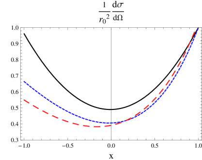
Figure 3: Differential cross section in the RS and NKR formalisms as a function of $x=\cos\theta$ for low values of the energy of the incident photon in the laboratory frame: $\eta=\omega/m$. The black curve corresponds to $\eta=0$ (Thomson limit), dashed curves correspond to $\eta=0.2$ in the NKR formalism (sort-dashed curve) and RS formalism (long-dashed curve).

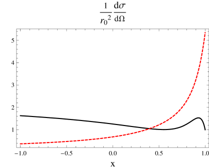
Figure 4: Differential cross section in the RS and NKR formalisms as a function of $x=\cos\theta$ for $\eta=1.5$. The solid curve corresponds to the results of the NKR formalism while the dashed curve are the results of the RS formalism.

The differential cross section reads

$$\frac{d\sigma_{NKR}}{d\Omega}=\frac{r_{0}^{2}}{(1+\eta z)^{7}}\sum_{n=0}^{10}h_{n}(z)\eta^{n}.$$ (88)

with $z=1-x$, $x=\cos\theta$ and

$$h_{0}(z) = \frac{1}{2}\left(z^{2}-2z+2\right),$$ (89)

$$h_{1}(z) = \frac{5}{2}z\left(z^{2}-2z+2\right),$$

$$h_{2}(z) = \frac{5}{2}z^{2}\left(2z^{2}-4z+5\right),$$

$$h_{3}(z) = 5z^{3}\left(z^{2}-2z+4\right),$$

$$h_{4}(z) = \frac{1}{18}z^{2}\left(45z^{4}-90z^{3}+384z^{2}+8z+18\right),$$

$$h_{5}(z) = \frac{1}{6}z^{3}\left(3z^{4}-6z^{3}+90z^{2}+8z+18\right),$$

$$h_{6}(z) = \frac{1}{162}z\left(1053z^{5}+297z^{4}+549z^{3}+108z^{2}-208z+64\right),$$

$$h_{7}(z) = \frac{1}{81}z^{2}\left(108z^{5}+117z^{4}+144z^{3}+108z^{2}-208z+64\right),$$

$$h_{8}(z) = \frac{1}{162}z^{3}\left(81z^{4}+63z^{3}+120z^{2}-256z+128\right),$$

$$h_{9}(z) = \frac{2}{81}z^{4}\left(3z^{2}-12z+16\right),$$

$$h_{10}(z) = \frac{8z^{5}}{81}.$$

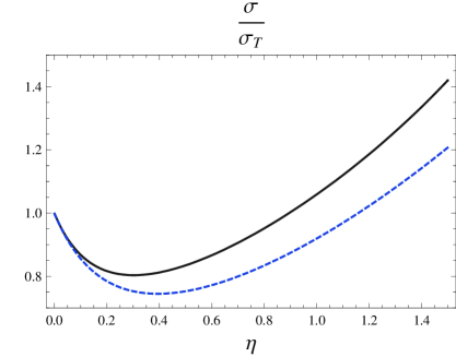
Figure 5: Total cross section normalized to the Thomson cross section. The solid line corresponds to the NKR formalism. The dashed curve is the result of the RS formalism.

In Fig. 3 we show the results of both formalisms for the differential cross section for low values of $\eta$. Although both formalisms coincide in the classical limit, even for values as low as $\eta=0.2$ there are sizable differences in the angular distribution of the emitted photons. For higher values of $\eta$ these differences become more important as shown in Fig. (4).

Integrating the solid angle we find the total cross section as

$$\sigma_{NKR} = \frac{\sigma_{T}}{3240\eta^{3}(2\eta+1)^{6}}[45(2\eta+1)^{6}\left(4\eta^{5}+21\eta^{4}-111\eta^{3}-153\eta^{2}-54\eta-54\right)\log(2\eta+1)$$ (90)

$$+ 2\eta(5376\eta^{12}-640\eta^{11}-15936\eta^{10}+14984\eta^{9}+516640\eta^{8}+1467750\eta^{7}+2010150\eta^{6}$$

$$+ 1742445\eta^{5}+1082160\eta^{4}+493830\eta^{3}+155115\eta^{2}+29160\eta+2430)].$$

The cross section normalized to the Thomson one is shown in Fig. (5) for $\eta\leq 1.5$ along with the result of the RS formalism in Eq. (IV). The NKR and RS formalisms yield the same result in the Thomson limit but their predictions for the total cross section differ beyond this point.

In the high energy limit the total cross section predicted by the NKR formalism grows as $\eta^{4}$. This is in contrast with the spin 1 case studied in NRDK where the total cross section remains finite in the high energy limit and further work is necessary in order to understand this point.

VI Summary and perspectives

In this work we study Compton scattering off a spin 3/2 elementary target in a recently proposed formalism for the description of high spin fields based on the Poincaré projectors and also in the conventional Rarita-Schwinger formalism. These formalisms yield the same result for the angular distribution and total cross section in the classical limit and coincide with the Thomson result. However, we obtain different predictions for these observables beyond this point, these differences becoming stronger at higher energies.

It is pointed out that the average squared amplitudes for Compton scattering in the forward direction for lower spin, ($s=0,1/2,1$), are energy independent and have the common value $4e^{4}$. In consequence, the differential cross sections in the forward direction and in the rest frame of the particles, coincide with the squared classical radius . This property is shared by the average squared amplitude for Compton scattering off spin $3/2$ particle as calculated in the Poincaré projector formalism but not in the Rarita-Schwinger formalism.

The classical regime tests only the lowest multipole (the electric charge), thus the differences in the angular distributions in these formalisms arise from the different predictions of these theories for higher multipoles and a calculation of these multipoles is desirable. Such analysis could also shed light on the high energy behavior of the total cross section. In contrast to the case of spin $1$ in the (1/2,1/2) representation space studied in NRDK which reproduces the electromagnetic couplings of the $W$ in the Standard Model and whose total cross section for Compton scattering remains finite at high energies, in the case of spin $3/2$ studied here it grows as $(\frac{\omega}{m})^{4}$ in this energy regime.

On the other hand, in the case of spin $1$ the Poincaré projectors automatically project onto subspaces with well defined parity. This is not the case for spin $3/2$ in whose case solutions with well defined parity must be chosen by hand. Therefore, it would be interesting to explore the consequences of a simultaneous projection onto well defined parity subspaces at the free particle level. Under $U(1)_{em}$ gauging we expect different predictions for the higher multipoles in this case.

VII Appendix

Our calculation yields the average squared amplitude

$$|\overline{\mathcal{M}}|^{2}=\frac{1}{324m^{10}\left(m^{2}-s\right)^{2}\left(m^{2}-u\right)^{2}}\sum_{n=0}^{9}{l_{2n}m^{2n}},$$ (91)

where

$$l_{0}= 2\left(f^{2}+gf+g^{2}\right)^{2}s^{2}u^{2}(s+u)\left(s^{2}+u^{2}\right)^{2},$$

$$l_{2}= 2\left(-5f^{4}+4(9-10g)f^{3}+4\left(-9g^{2}+6g+7\right)f^{2}-4g(g(g+12)-16)f+4g^{2}((g-12)g+16)\right)s^{4}u^{4}$$

$$-\left(25f^{4}+(92g-52)f^{3}+6(g(25g-16)-2)f^{2}+8g(g(19g-24)+6)f+4g^{2}(g(19g-32)+12)\right)$$

$$\times s^{3}\left(s^{2}+u^{2}\right)u^{3}-4\left(f^{2}+gf+g^{2}\right)\left(6f^{2}+6(3g-2)f+3g(5g-4)-4\right)s^{2}\left(s^{4}+u^{4}\right)u^{2}$$

$$-4\left(f^{2}+gf+g^{2}\right)^{2}s\left(s^{6}+u^{6}\right)u$$

$$l_{4}= (s+u)\left(-2\left(17f^{4}+4(38-17g)f^{3}+\left(-303g^{2}+852g-504\right)f^{2}+4(g(7(27-5g)g-276)+80)f\right.\right.$$

$$\left.\left.-4(g(g(g(7g-136)+357)-316)+116)\right)s^{3}u^{3}+\left(95f^{4}+14(35g-32)f^{3}+(3g(441g-596)+448)f^{2}\right.\right.$$

$$\left.\left.+4(g(g(316g-459)+94)+24)f+2(g(g(g(277g-592)+518)-504)+328)\right)\left(u^{2}s^{4}+u^{4}s^{2}\right)\right.$$

$$\left.+2\left(f^{2}+gf+g^{2}\right)\left(17f^{2}-36f+44g^{2}+8(7f-3)g-28\right)\left(us^{5}+u^{5}s\right)+2\left(f^{2}+gf+g^{2}\right)^{2}\left(s^{6}+u^{6}\right)\right)$$

$$l_{6}= -2\left(185f^{4}+2(899g-1126)f^{3}+(69g(83g-156)+4996)f^{2}+4(g(g(1210g-2709)+2272)-388)f\right.$$

$$\left.+g(g(g(2291g-9592)+15856)-10448)+2976\right)s^{3}u^{3}-\left(447f^{4}+30(93g-106)f^{3}+2\left(4443g^{2}\right.\right.$$

$$\left.\left.-7332g+2846\right)f^{2}+4(g(3g(653g-1150)+2062)-352)f+16(g(g(3g(76g-231)+892)-554)\right.$$

$$\left.+200)\right)\left(u^{2}s^{4}+u^{4}s^{2}\right)-\left(206f^{4}+(826g-736)f^{3}+(3g(739g-844)+584)f^{2}+4(g(g(460g-387)\right.$$

$$\left.-16)+60)f+g(g(g(941g-1592)+968)-912)+1120\right)\left(us^{5}+u^{5}s\right)$$

$$-2\left(f^{2}+gf+g^{2}\right)\left(16g^{2}+22fg+f(7f-12)-20\right)\left(s^{6}+u^{6}\right)$$

$$l_{8}= (s+u)\left(2\left(388f^{4}+(3446g-4020)f^{3}+2\left(5079g^{2}-9216g+4054\right)f^{2}+8\left(1165g^{3}-2610g^{2}+1792g\right.\right.\right.$$

$$\left.\left.\left.-190\right)f+4849g^{4}-15312g^{3}+18704g^{2}-7984g+1568\right)s^{2}u^{2}+2\left(349f^{4}+2(679g-836)f^{3}\right.\right.$$

$$\left.\left.+\left(5175g^{2}-7392g+3232\right)f^{2}+4\left(1013g^{3}-1320g^{2}+532g+80\right)f+2278g^{4}-4628g^{3}+4492g^{2}\right.\right.$$

$$\left.\left.-1856g+560\right)\left(us^{3}+u^{3}s\right)+\left(116f^{4}+(202g-268)f^{3}+6\left(151g^{2}-84g+6\right)f^{2}\right.\right.$$

$$\left.\left.+8\left(56g^{3}-27g^{2}-6g+18\right)f+389g^{4}-272g^{3}+540g^{2}-768g+752\right)\left(s^{4}+u^{4}\right)\right)$$

$$l_{10}= -2\left(1177f^{4}+22(359g-386)f^{3}+(3g(9953g-14396)+15572)f^{2}+4(g(g(6491g-11139)+3668)\right.$$

$$\left.+2252)f+g(g(g(13105g-20512)+5072)+9424)-4992\right)s^{2}u^{2}-\left(1647f^{4}+36(187g-223)f^{3}\right.$$

$$\left.+2(27g(617g-768)+7726)f^{2}+8\left(g\left(3177g^{2}-4362g+994\right)+1376\right)f+2\left(g\left(g\left(6705g^{2}-8688g\right.\right.\right.\right.$$

$$\left.\left.\left.\left.+3604\right)+2800\right)-1408\right)\right)\left(us^{3}+u^{3}s\right)+\left(-416f^{4}-26(5g-28)f^{3}-(9g(515g-268)+160)f^{2}\right.$$

$$\left.-4(g(g(463g-249)+316)+76)f-g(g(g(1517g-976)+2080)-1552)-736\right)\left(s^{4}+u^{4}\right)$$

$$l_{12}= \left(255f^{4}+2(2409g-928)f^{3}+\left(55731g^{2}-48972g+5904\right)f^{2}+4\left(10989g^{3}-9339g^{2}-5418g+8632\right)f\right.$$

$$\left.+2\left(6489g^{4}+5212g^{3}-24534g^{2}+21064g+1736\right)\right)\left(us^{2}+u^{2}s\right)+\left(301f^{4}-2(653g-544)f^{3}\right.$$

$$\left.+9\left(1425g^{2}-388g-336\right)f^{2}+4\left(1511g^{3}+231g^{2}+258g-72\right)f\right.$$

$$\left.+1414g^{4}+2632g^{3}-4404g^{2}+4080g-784\right)\left(s^{3}+u^{3}\right)$$

$$l_{14}= 2\left(1699f^{4}+4(908g-2063)f^{3}-84\left(276g^{2}-44g-75\right)f^{2}-16\left(1108g^{3}+603g^{2}-1536g+450\right)f\right.$$

$$\left.+2\left(1649g^{4}-11240g^{3}+14328g^{2}-5376g-7616\right)\right)su+\left(1361f^{4}+(5488g-8756)f^{3}-4\left(4854g^{2}\right.\right.$$

$$\left.\left.+1056g-2321\right)f^{2}-16\left(704g^{3}+1035g^{2}-473g-608\right)f\right.$$

$$\left.+2\left(2407g^{4}-8072g^{3}+8584g^{2}-2848g-96\right)\right)\left(s^{2}+u^{2}\right)$$

$$l_{16}= -4\left(735f^{4}+(2178g-3704)f^{3}+(1688-33g(111g+124))f^{2}+4(g(566-3g(197g+735))+2020)f\right.$$

$$\left.+g(g(g(3033g-5308)+926)+4184)+2952\right)(s+u)$$

$$l_{18}= 12\left(139f^{4}+(398g-668)f^{3}-3\left(117g^{2}+316g+20\right)f^{2}-4\left(55g^{3}+450g^{2}+54g-628\right)f\right.$$

$$\left.+4\left(157g^{4}-154g^{3}-189g^{2}+404g+652\right)\right)$$ (92)

This amplitude is clearly symmetric under the $s\leftrightarrow u$ exchange.

References

• (1) W. Rarita, J. Schwinger, Phys. Rev. 60, 61 (1941).
• (2) K. Johnson, E. C. Sudarshan, Annals of Physics  13, 126 (1961).
• (3) G. Velo, D. Zwanziger, Phys. Rev. 186, 1337 (1969); Phys. Rev. 188, 2218 (1969).
• (4) L. M. Nath, B. Etemadi, J. D. Kimel, Phys. Rev. D 3, 2153 (1971); R. Davidson, N. C. Mukhopadhyay, R. S. Wittman, Phys. Rev. D 43, 71 (1991); M. Napsuciale, J. L. Lucio, Phys. Lett. B 384, 227 (1996); ibid., Nucl. Phys. B494, 260 (1997).
• (5) M. Napsuciale, M. Kirchbach and S. Rodriguez, Eur. Phys. J.  A 29, 289 (2006) [arXiv:hep-ph/0606308].
• (6) S. D. Drell, A.  Hearn, Phys. Rev. Lett. 16, 908 (1966); S. B. Gerasimov, Sov. J. Nucl. Phys. 2, 430 (1966): Yad. Fis. 2, 598 (1966); S. Weinberg, in Lectures on Elementary Particles and Quantum Field Theory, Edited by S. Deser et.al. (MIT Press, Cambridge, Mass, 1971, Vol I); S. Ferrara, M. Porrati, V. Telegdi, Phys. Rev. D 46, 3529 (1992); B. R. Holstein, Phys. Rev.  D 74, 085002 (2006); Am. J. Phys. 74, 1104 (2006); C. Lorce, Phys. Rev.  D 79, 113011 (2009) [arXiv:0901.4200 [hep-ph]].
• (7) M. Napsuciale, S. Rodriguez, E. G. Delgado-Acosta and M. Kirchbach, Phys. Rev.  D 77, 014009 (2008) [arXiv:0711.4162 [hep-ph]].
• (8) K. Hagiwara, R. Peccei, D. Zeppenfeld and K. Hikasa, Nucl. Phys. B282 (1987) 253; arXiv:hep-ex/0102041v1 DELPHI Coll.
• (9) F. J. Belinfante, Phys. Rev.  92, 997 (1953); J. Mathews, Phys. Rev. 102, 270,1956; A. Pais, Phys. Rev. Lett.  19, 544 (1967); V. Singh, Phys. Rev. Lett.  19, 730 (1967); J. S. Bell, Nuovo Cimento 52 A, 635 (1967); I. J. Kalet, Phys. Rev.  176, 2135 (1968); K. Bardakci and H. Pagels, Phys. Rev.  166, 1783 (1968); S. Saito, Phys. Rev. 184, 1984 (1969); G. F. Leal Ferreira and S. Ragusa, Nuovo Cim.  A 65, 607 (1970); S. Ragusa, Phys. Rev.  D 8, 1190 (1973); S. Ragusa, Phys. Rev.  D 29, 2636 (1984); R. Cuevas and A Queijeiro, Rev. Mex. Fís. 48, 271 (2002); V. Pascalutsa, M. Vanderhaeghen and S. N. Yang, Phys. Rept.  437, 125 (2007) [arXiv:hep-ph/0609004]; V. Pascalutsa, Nucl. Phys.  A 680, 76 (2000) [arXiv:nucl-th/0005006]; M. Porrati and R. Rahman, Phys. Rev.  D 80, 025009 (2009) [arXiv:0906.1432 [hep-th]].
• (10) Haryanto M. Siahaan, Triyanta, Indonesian Journal of Physics 19, 51 (2008).
• (11) S. Kamefuchi, L. O’Raifeartaigh, A. Salam, Nucl. Phys. 28, 529 (1961).
• (12) K. Dormuth and R. Teshima, Lettere al Nuovo Cimento IV, 796 (1970).