Experimental criteria for steering and the Einstein-Podolsky-Rosen paradox

Abstract

We formally link the concept of steering (a concept created by Schrödinger but only recently formalised by Wiseman, Jones and Doherty [Phys. Rev. Lett. 98, 140402 (2007)] and the criteria for demonstrations of Einstein-Podolsky-Rosen (EPR) paradox introduced by Reid [Phys. Rev. A, 40, 913 (1989)]. We develop a general theory of experimental EPR-steering criteria, derive a number of criteria applicable to discrete as well as continuous-variables observables, and study their efficacy in detecting that form of nonlocality in some classes of quantum states. We show that previous versions of EPR-type criteria can be rederived within this formalism, thus unifying these efforts from a modern quantum-information perspective and clarifying their conceptual and formal origin. The theory follows in close analogy with criteria for other forms of quantum nonlocality (Bell-nonlocality and entanglement), and because it is a hybrid of those two, it may lead to insights into the relationship between the different forms of nonlocality and the criteria that are able to detect them.

I Introduction

In their seminal 1935 paper (Einstein1935, ), Einstein, Podolsky and Rosen (EPR) presented an argument which demonstrates the incompatibility between the concepts of local causality and the completeness of quantum mechanics. Apart from the foundational importance of that work, it had long-reaching consequences (Vedral2006, ): it was the first time that physicists clearly noticed the strange phenomena associated with entanglement — the resource at the basis of modern quantum information science.

The situation depicted by EPR is often referred to as the “EPR paradox”. The authors themselves did not intend to point out a true paradox; instead they argued that quantum mechanics was an incomplete theory, that is, that it did not give a complete description of reality. Schrödinger (SchPCP35, ) seems to have been the first to name the situation a ‘paradox’, as he could not believe with EPR that quantum mechanics was indeed incomplete but neither could he see a flaw in the argument. In hindsight, we now know (since Bell (Bell1964, )) that, while the argument is sound, one of the premises — local causality — is false. However, we will retain the historically prevalent term ‘paradox’, if only because we still do not have a fully satisfactory understanding of the nature of quantum nonlocality.

The original EPR paradox involved an example of an idealized bipartite entangled state of continuous variables measured at the two subsystems. Later, Bohm (Bohm1951, ) extended the EPR paradox to a scenario involving discrete (spin) observables. The essence of both of these arguments involved perfect correlations, and therefore neither the original EPR paradox nor Bohm’s version could be directly tested in the laboratory without additional assumptions. Criteria for the experimental demonstration of the EPR paradox, which can be used in situations with non-ideal states, have been derived for the continuous-variables scenario by Reid in 1989 (Reid1989, ) and more recently for discrete systems by Cavalcanti and Reid (Cavalcanti2007b, ) and Cavalcanti et al. (Cavalcanti2009b, ).

In another recent development, Wiseman, Jones and Doherty (Wiseman2007, ) have introduced a new classification of quantum nonlocality, a formalisation of the concept of steering introduced by Schrödinger in 1935 (Schroedinger1935, ) in a response to the EPR paper. In that Letter, the authors claimed that any demonstration of the EPR paradox, as proposed by Reid, is also a demonstration of steering. While that claim was essentially correct, the proof proposed there was incomplete, as we will see later in this paper. We will provide the missing proof and further show that the converse is also true: any demonstration of steering is also a demonstration of the EPR paradox. In other words, the EPR paradox and steering are equivalent notions of nonlocality.

In Ref. (Wiseman2007, ) Wiseman, Jones and Doherty showed that EPR-steering constitutes a different class of nonlocality intermediate between the classes of quantum non-separability and Bell-nonlocality, with the distinction between these being explainable as a matter of trust between different parties. Therefore, besides its foundational interest, this classification could prove important in the context of quantum communication and information. It would be thus desirable to devise criteria to determine to which classes a given state (or a set of observed correlations) belongs. For that purpose we will formulate and develop the theory of EPR-steering criteria, defined as any criteria which are sufficient to demonstrate EPR-steering experimentally. The theory will proceed in close analogy to the theories of entanglement criteria (Duan2000, ; Simon2000, ; Hofmann2003a, ; Guhne2004a, ) and of Bell inequalities (or Bell-nonlocality criteria) (Bell1964, ; Clauser1969, ; Mermin1980, ; Fine1982, ; Pitowsky1989, ; Ardehali1992, ; Belinskii1993, ; Peres1999, ; Werner2001, ; Collins2002a, ; Zukowski2002a, ; Cavalcanti2007a, ).

The structure of the paper is as follows: In Sec. II we will review some of the history and concepts surrounding the EPR paradox and steering. The main purposes of this section are to review the conceptual motivation for the new formulation and to put the steering criteria proposed here in context with the relevant literature. In Sec. III we will review the three classes of nonlocality, including Wiseman and coworkers’ (Wiseman2007, ) steering, and argue in more detail than in previous papers (Jones2007, ) as to why it provides the correct formalization of Schrödinger’s concept. In Sec. IV we will introduce the formalism for derivation of general EPR-steering criteria. We develop two broad classes of EPR-steering criteria: the multiplicative variance criteria, and the additive convex criteria (which includes linear EPR-steering inequalities as a special case). We show how the criteria in the existing literature can be rederived as special cases within this modern unifying approach. In Sec. V we will apply the criteria derived in Sec. IV to some classes of quantum states, comparing their effectiveness in experimentally demonstrating EPR-steering. We consider both continuous variables (as in the original EPR paradox) and spin-half systems (as in Bohm’s version).

II History and concepts

II.1 The Einstein-Podolsky-Rosen argument

The EPR argument has been exhaustively commented in the literature. However, since in this paper we will discuss a new mathematical formulation of it, it will be important to review it in detail.

The essence of Einstein and coworkers’ (Einstein1935, ) 1935 argument is a demonstration of the incompatibility between the premises of local causality and the completeness of quantum mechanics. EPR started the paper by making a distinction between reality and the concepts of a theory, followed by a critique of the operationalist position, clearly aimed at the views advocated by Bohr, Heisenberg and the other proponents of the Copenhagen interpretation.

“Any serious consideration of a physical theory must take into account the distinction between the objective reality, which is independent of any theory, and the physical concepts with which the theory operates. These concepts are intended to correspond with the objective reality, and by means of these concepts we picture this reality to ourselves.

In attempting to judge the success of a physical theory, we may ask ourselves two questions: (1) ‘Is the theory correct?’ and (2) ‘Is the description given by the theory complete?’ It is only in the case in which positive answers may be given to both of these questions, that the concepts of the theory may be said to be satisfactory.” (Einstein1935, )

Any theory will have some concepts which will be used to aid in the description and prediction of the phenomena which are their subject matter. In quantum theory, Schrödinger introduced the concept of the wave function and Heisenberg described the same phenomena with the more abstract matrix mechanics. EPR argued that we must distinguish those concepts from the reality they attempt to describe. One can see the physical concepts of the theory as mere calculational tools if one wishes, but it was those authors’ opinion that one must be careful to avoid falling back into a pure operationalist position; the theory must strive to furnish a complete picture of reality.

EPR follow the previous considerations with a necessary condition for completeness:

EPR’s necessary condition for completeness: “Whatever the meaning assigned to the term complete, the following requirement for a complete theory seems to be a necessary one: every element of the physical reality must have a counterpart in the physical theory.” (Einstein1935, )

Soon afterward they note that this condition only makes sense if one is able to decide what are the elements of the physical reality. They did not attempt to define ‘element of physical reality’, saying “The elements of the physical reality cannot be determined by a priori philosophical considerations, but must be found by an appeal to results of experiments and measurements. A comprehensive definition of reality is, however, unnecessary for our purpose”. Instead they provide a sufficient condition:

EPR’s sufficient condition for reality: We shall be satisfied with the following criterion, which we regard as reasonable. If, without in any way disturbing a system, we can predict with certainty (i.e., with probability equal to unity) the value of a physical quantity, then there exists an element of physical reality corresponding to this physical quantity.” (Einstein1935, )

Later in the same paragraph it is made explicit that this criterion is “regarded not as a necessary, but merely as a sufficient, condition of reality”. This is followed by a discussion to the effect that, in quantum mechanics, if a system is in an eigenstate of an operator $A$ with eigenvalue $a$, by this criterion, there must be an element of physical reality corresponding to the physical quantity $A$. “On the other hand”, they continue, if the state of the system is a superposition of eigenstates of $A$, “we can no longer speak of the physical quantity $A$ having a particular value”. After a few more considerations, they state that “the usual conclusion from this in quantum mechanics is that when the momentum of a particle is known, its coordinate has no physical reality”. We are left therefore, according to EPR, with two alternatives:

EPR’s dilemma: “From this follows that either (1) the quantum-mechanical description of reality given by the wave function is not complete or (2) when the operators corresponding to two physical quantities do not commute the two quantities cannot have simultaneous reality.” (Einstein1935, )

They justify this by reasoning that “if both of them had simultaneous reality — and thus definite values — these values would enter into the complete description, according to the condition for completeness”. And in the crucial step of the reasoning: “If then the wave function provided such a complete description of reality it would contain these values; these would then be predictable [our emphasis]. This not being the case, we are left with the alternatives stated”. Brassard and Méthot (Brassard2006, ) (correctly) pointed out that strictly speaking EPR should conclude that (1) or (2), instead of either (1) or (2), since they could not exclude the possibility that (1) and (2) could be both correct. However, this does not affect EPR’s conclusion. It was enough for them to show that (1) and (2) could not both be wrong, and therefore if one can find a reason for (2) to be false, (1) must be true .

The next section in EPR’s paper intends to find a reason for (2) to be false, that is, to find a circumstance in which one can say that there are simultaneous elements of reality associated to two non-commuting operators. They consider a composite system composed of two spatially separated subsystems $S_{A}$ and $S_{B}$ which is prepared, by way of a suitable initial interaction, in an entangled state of the type

$$|\Psi\rangle=\sum_{n}c_{n}|\psi_{n}\rangle_{A}\otimes|u_{n}\rangle_{B},$$ (1)

where the $|\psi_{n}\rangle_{A}$ denote a basis of eigenstates of an operator, say $\hat{O}_{1}$, of subsystem $S_{A}$ and $|u_{n}\rangle_{B}$ denote some (normalised but not necessarily orthogonal) states of $S_{B}$. If one measures the quantity $\hat{O}_{1}$ at $S_{A}$, and obtains an outcome corresponding to eigenstate $|\psi_{k}\rangle_{A}$ the global state is reduced to $|\psi_{k}\rangle_{A}\otimes|u_{k}\rangle_{B}$. If, on the other hand, one chooses to measure a non-commuting observable $\hat{O}_{2}$, with eigenstates $|\phi_{s}\rangle_{A}$, one should instead use the expansion

$$|\Psi\rangle=\sum_{s}c^{\prime}_{s}|\phi_{s}\rangle_{A}\otimes|v_{s}\rangle_{B},$$ (2)

where $|v_{s}\rangle_{B}$ represent, in general, another set of states of $S_{B}$. Now if the outcome of this measurement is, say, the one corresponding to $|\phi_{r}\rangle_{A}$, the global state is thereby reduced to $|\phi_{r}\rangle_{A}\otimes|v_{r}\rangle_{B}$. Therefore, “as a consequence of two different measurements performed upon the first system, the second system may be left in states with two different wave functions”. This is just what Schrödinger later termed steering, and we will return to that later. Now enters the crucial assumption of locality, justified by the fact that the systems are spatially separated and thus no longer interacting.

EPR’s necessary condition for locality: “No real change can take place in the second system in consequence of anything that may be done to the first system.” (Einstein1935, )

Einstein et al. never explicitly used the term ‘locality’, but took this assumption for granted. Because of this we call this a “necessary condition for locality”, as this is the most conservative reading of EPR’s reasoning: if they had explicitly defined some assumption of locality, this would certainly be an implication of it, but there is no reason (and no need) to take it as a definition.

“Thus”, conclude EPR, “it is possible to assign two different wave functions to the same reality”. EPR could have now simply concluded by noting that two different (pure) states can in general assign unit probability (and thus an element of reality, according to the locality assumption and the sufficient condition for reality) to each of two non-commuting quantities, in contradiction of statement (2); this would imply, by way of EPR’s dilemma, that quantum mechanics is incomplete. Instead, they consider a specific example, depicted in Fig. 1, where those different wave functions are respective eigenstates of position and momentum. Because they are canonically conjugate, this guarantees that $|u_{n}\rangle$ is different from $|v_{s}\rangle$ for every possible outcome n or s. The paradox is thus guaranteed to be realised — one cannot attempt to hide behind statistics. If the initial state was of type

$$\Psi(x_{A},x_{B})=\int_{-\infty}^{\infty}e^{ix_{A}p/\hbar}e^{-ix_{B}p/\hbar}dp,$$ (3)

then if one measures momentum $\hat{p}^{A}$ at $S_{A}$ and finds outcome $p$, the reduced state of subsystem $S_{B}$ will be the one associated with outcome $-p$ of $\hat{p}^{B}$. On the other hand, if one measures position $\hat{x}^{A}$ and finds outcome $x$, the reduced state of $S_{B}$ will be the one corresponding to outcome $x$ of $\hat{x}^{B}$. By measuring position or momentum at $S_{A}$, one can predict with certainty the outcome of the same measurement on $S_{B}$. But $\hat{p}^{B}$ and $\hat{x}^{B}$ correspond to non-commuting operators. EPR conclude from this that

“In accordance with our criterion of reality, in the first case we must consider the quantity [$\hat{p}^{B}$] as being an element of reality, in the second case the quantity [$\hat{x}^{B}$] is an element of reality. But, as we have seen, both wave functions [corresponding to $-p$ and $x$] belong to the same reality.” (Einstein1935, )

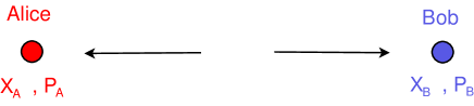
Figure 1: The EPR scenario. Alice and Bob are two spatially separated observers who can perform one of two (position or momentum) measurements available to each of them.

In other words, by using the sufficient condition for reality, the necessary condition for locality and the predictions for the entangled state under consideration, EPR conclude that there must be elements of reality associated to a pair of non-commuting operators. So horn (2) of EPR’s dilemma is closed, leaving as the only alternative option (1), namely, that the quantum mechanical description of physical reality is incomplete.

In more modern terminology, the conclusion of EPR was to infer the existence of a set of local hidden variables (LHVs) underlying quantum systems which should be able to reproduce the statistics. It is trivial to reproduce the statistics of EPR’s example with LHVs, even though that is not possible with some entangled states, as later proved by Bell (Bell1964, ). Schrödinger arrived at a different conclusion from an analysis of the paradox raised by EPR, as we will see in the next section.

In hindsight, as we now know that the premise of locality is not justified, we can read EPR’s argument as demonstrating the incompatibility between the premises of locality, the completeness of quantum mechanics and some of its predictions.

II.2 Schrödinger’s response: The concept of steering

EPR’s argument prompted an interesting response from Schrödinger (SchPCP35, ; Schroedinger1935, ). He also considered nonfactorizable pure states describable by the wave function given by Eq. (1). Schrödinger, however, had of course developed the wave function for atoms and believed that it gave a complete description of a quantum system. So while he was not prepared to accept EPR’s conclusion that quantum mechanics was incomplete, neither could he see a flaw with their argument. For this reason he termed the situation described by EPR a paradox.

Clearly Schrödinger was also interested in implications arising from composite quantum systems described by nonfactorizable pure states. He described this situation, coining a famous term, as follows: “If two separated bodies, each by itself known maximally, enter a situation in which they influence each other, and separate again, then there occurs regularly … [an] entanglement of our knowledge of the two bodies.” (SchPCP35, )

Having defined entanglement, Schrödinger then defined the process of disentanglement which occurs when a non-degenerate observable is measured on one body: “After establishing one representative by observation, the other one can be inferred simultaneously … this procedure will be called the disentanglement”. This leads us directly to the EPR paradox, as Schrödinger describes it:

“[EPR called attention] to the obvious but very disconcerting fact that even though we restrict the disentangling measurements to one system, the representative obtained for the other system is by no means independent of the particular choice of observations which we select for that purpose and which by the way are entirely arbitrary.” (SchPCP35, )

Schrödinger describes this ability to affect the state of the remote subsystem as steering:

“It is rather discomforting that the theory should allow a system to be steered or piloted into one or the other type of state at the experimenter’s mercy in spite of his having no access to it.” (SchPCP35, )

EPR’s example concerning position and momentum was recast in the context of steering as

“Since I can predict either $x_{1}$ or $p_{1}$ without interfering with system No. 1 and since system No. 1, like a scholar in examination, cannot possibly know which of the two questions I am going to ask it first: it so seems that our scholar is prepared to give the right answer to the first question he is asked anyhow. He must know both answers; which is an amazing knowledge.” (SchPCP35, )

The remainder of Schrödinger’s paper is a generalisation of steering to more than two measurements:

“[System No. 1] does not only know these two answers but a vast number of others, and that with no mnemotechnical help whatsoever, at least none that we know of.” (SchPCP35, )

By “mnemotechnical help” Schrödinger presumably means a cheat-sheet (to use his scholar analogy). That is, a set of local hidden variables (LHVs) that determine the measurement results. Thus, unlike EPR, Schrödinger explicitly rejected LHVs as an explanation of steering. Perhaps because he had performed explicit calculations generalizing EPR’s example (which can be explained trivially using LHVs), he recognized steering as “a necessary and indispensable feature” (SchPCP36, ) of quantum mechanics. We now know, thanks to Bell’s theorem, that Schrödinger’s intuition was correct: there is no possible local hidden variable model (or local mnemotechnical help) to explain the correlations between measurement outcomes for certain entangled states (Gisin1991, ).

Like EPR, Schrödinger was troubled by the implications of steerability of entangled states for quantum theory. Unlike EPR, however, he saw the resolution of the paradox lying in the incorrectness of the predictions of quantum mechanics. That is, he was “not satisfied about there being sufficient experimental evidence for” steering in nature (SchPCP36, ). This raises the obvious question: what evidence would have convinced Schrödinger? The pure entangled states he discussed are an idealization, so we cannot expect ever to observe precisely the phenomenon he introduced. On the other hand, Schrödinger was quite explicit that a separable but classically correlated state which allows “determining the state of the first system by suitable measurement of the second or vice versa” (SchPCP36, ) could never exhibit steering. For this situation, he says that “it would utterly eliminate the experimenter’s influence on the state of that system which he does not touch.” (SchPCP36, ). Thus it is apparent that by steering Schrödinger meant something that could not be explained by Alice simply finding out which state Bob’s system is in, out of some predefined ensemble of states. Following this reasoning leads to the general definition of steering as presented in Ref. (Wiseman2007, ). We return to this concept in Sec. III.

II.3 Bohm’s version

Although making reference to a general entangled state, the original EPR argument used the specific case of a continuous-variable state for its final (and crucial) part. In his 1951 textbook (Bohm1951, ), Bohm presented a discussion of the EPR paradox in a modified scenario involving two entangled spin-1/2 particles. Although trivial in hindsight, this extension had a fundamental importance. It was the scenario used by Bell in the proof of his now famous theorem (Bell1964, ) and for most of the subsequent discussions of Bell inequalities (a Bell-type inequality directly applicable to continuous-variables has only recently been derived (Cavalcanti2007a, )), and was instrumental for our present understanding of entanglement, and particularly for its applications in quantum information processing.

In Bohm’s version the system of interest is a molecule containing two spin-1/2 atoms in a singlet state, in which the total spin is zero:

$$|\Psi_{s}\rangle=|z_{+}\rangle_{A}\otimes|z_{-}\rangle_{B}-|z_{-}\rangle_{A}\otimes|z_{+}\rangle_{B}.$$ (4)

Here $|z_{\pm}\rangle$ represent the $\pm 1/2$ eigenstate of the spin projection operator along the z direction, $S_{z}$. Compare this state with Eq. (1) used in the EPR argument. If $S_{z}$ is measured on system A, and the outcome corresponding to $|z_{+}\rangle_{A}$ (or $|z_{-}\rangle_{A}$) is obtained, the state of subsystem B is projected into $|z_{-}\rangle_{B}$ (or $|z_{+}\rangle_{B}$). Thus, one predicts an element of reality for the $z$ component of the spin of the second atom. But the same state can be written, in the basis of eigenstates of another spin projection, say $S_{x},$

$$|\Psi_{s}\rangle=|x_{+}\rangle_{A}\otimes|x_{-}\rangle_{B}-|x_{-}\rangle_{A}\otimes|x_{+}\rangle_{B}.$$ (5)

Similarly, the $x$ component of the spin of the first atom could be measured instead, allowing inference of an element of reality associated with the $x$ component of spin for the second atom. With this mapping, the rest of the argument follows in analogy with EPR’s.

Bohm’s version of the EPR paradox is conceptually appealing, but (in his 1951 textbook at least) he did not present it as an argument for the incompleteness of quantum theory (as did EPR). Instead, he used it to argue that a complete description of nature need not contain a one-to-one correspondence between elements of reality and the mathematical description provided by the theory. Bohm defended, in 1951, the interpretation that the quantum state represents only “potentialities” of measurement results, which actually occur only when a system interacts with an appropriate apparatus. It is curious to find that already in 1952 Bohm must have found this interpretation wanting, since he then developed his famous non-local hidden-variable interpretation of quantum mechanics (Bohm1952a, ; Bohm1952b, ), where there is such a one-to-one correspondence.

As the original continuous-variable example remained unrealizable for decades, several early experiments followed Bohm’s proposal, such as Bleuler and Bradt (1948) (Bleuler1948, ), Wu and Shaknov (1950) (Wu1950, ) and Kocher and Commins (1967) (Kocher1967, ). All of these suffered from low detection efficiencies and had no concern with causal separation, however, making their interpretation debatable.

II.4 The EPR-Reid criterion

While the EPR argument was logically sound, one could block its conclusion by rejecting those statistical predictions required to formulate it. As we have discussed in Sec. II.2, Schrödinger seems to have found this an appealing solution. This move is particularly easy to make since the necessary predictions are of perfect correlations, unobtainable in practice due to unavoidable inefficiency in preparation and detection of real physical systems. This problem was considered by Furry already in 1936 (Furry1936, ) but experimentally useful criteria for the EPR paradox were only proposed in 1989 by Reid (Reid1989, ), which we will discuss in detail later in this section. The notation and terminology will closely follow that of a recent review on the EPR paradox (Reid2008tb, ). The essential difference in the derivation of the EPR-Reid criteria and the original EPR argument is in a modification of the sufficient condition for reality . This could be stated as the following:

Reid’s extension of EPR’s sufficient condition of reality: If, without in any way disturbing a system, we can predict with some specified uncertainty the value of a physical quantity, then there exists a stochastic element of physical reality which determines this physical quantity with at most that specific uncertainty.

The scenario considered is the same as the one for the EPR paradox above, as depicted in Fig. 1, but one does not need a state which predicts the perfect correlations considered by EPR. Instead, the two experimenters, Alice and Bob, can measure the conditional probabilities of Bob finding outcome $x_{B}$ in a measurement of $\hat{x}_{B}$ given that Alice finds outcome $x_{A}$ in a measurement of $\hat{x}_{A}$, i.e., $P(x_{B}|x_{A})$. Similarly they can measure the conditional probabilities $P(p_{B}|p_{A})$ and the unconditional probabilities $P(x_{A})$, $P(p_{A})$. We denote by $\Delta^{2}(x_{B}|x_{A})$, $\Delta^{2}(p_{B}|p_{A})$ the variances of the conditional distributions $P(x_{B}|x_{A})$, $P(p_{B}|p_{A})$, respectively. Based on a result $x_{A},$ Alice can make an estimate of the result for Bob’s outcome $x_{B}.$ Denote this estimate $x_{B}^{{\rm est}}(x_{A}).$ The average inference variance of $x_{B}$ given estimate $x_{B}^{{\rm est}}(x_{A})$ is defined as

$$\Delta_{\mathrm{inf}}^{2}x_{B}\equiv\langle(x_{B}-x_{B}^{{\rm est}}(x_{A}))^{2}\rangle\\ =\int dx_{A}dx_{B}P(x_{A},x_{B})(x-x_{B}^{{\rm est}}(x_{A}))^{2}.$$ (6)

Note that this average inference variance is minimized when the estimate is just the expectation value of $x_{B}$ given $x_{A},$ i.e., the mean of the distribution $P(x_{B}|x_{A})$ (Reid2008tb, ). Therefore the optimal (or minimum) inference variance of $x_{B}$ ($p_{B}$) given a measurement $\hat{x}_{A}$ ($\hat{p}_{A}$) is given by

$$\Delta_{\mathrm{min}}^{2}x_{B} = \mathrm{min}_{x_{B}^{{\rm est}}}\{\Delta_{\mathrm{inf}}^{2}x_{B}\}$$ (7)

$$= \int dx_{A}dx_{B}P(x_{A})\Delta^{2}(x_{B}|x_{A});$$

$$\Delta_{\mathrm{min}}^{2}p_{B} = \mathrm{min}_{p_{B}^{{\rm est}}}\{\Delta_{\mathrm{inf}}^{2}p_{B}\}$$ (8)

$$= \int dp_{A}dp_{B}P(p_{A})\Delta^{2}(p_{B}|p_{A}).$$

Reid showed, by use of the sufficient condition of reality above, that since Alice can, by measuring either position $\hat{x}_{A}$ or momentum $\hat{p}_{B}$, infer with some uncertainty $\Delta_{\mathrm{inf}}x_{B}=\sqrt{\Delta_{\mathrm{inf}}^{2}x_{B}}$ or $\Delta_{\mathrm{inf}}p_{B}=\sqrt{\Delta_{\mathrm{inf}}^{2}p_{B}}$ the outcomes of the corresponding experiments performed by Bob, and since by the locality condition of EPR her choice cannot affect the elements of reality of Bob, then there must be simultaneous stochastic elements of reality which determine $\hat{x}_{B}$ and $\hat{p}_{B}$ with at most those uncertainties. Now by Heisenberg’s Uncertainty Principle (HUP), quantum mechanics imposes a limit to the precision with which one can assign values to observables corresponding to non-commuting operators such as $\hat{x}$ and $\hat{p}$. In appropriately rescaled units the relevant HUP reads $\Delta x\Delta p\geq 1$. Therefore, if quantum mechanics is complete and the locality condition holds, by use of the extended sufficient condition of reality and EPR’s necessary condition for completeness, the limit with which one could determine the average inference variances above is

$$\Delta_{\mathrm{inf}}x_{B}\Delta_{\mathrm{inf}}p_{B}\geq 1.$$ (9)

This is the EPR-Reid criterion. Violation of that criterion signifies the EPR paradox, and has been experimentally demonstrated in continuous-variables quantum optics experiments with quadratures (Ou1992, ; Zhang2000, ; Silberhorn2001, ; Schori2002, ; Bowen2003, ) and actual position-momentum measurements (Howell2004, ). While these were performed with high detection efficiency, none of these experimental demonstrations have been able to achieve causal separation between the measurements. For a detailed review see (Reid2008tb, ).

II.5 Recent developments

Cavalcanti and Reid (Cavalcanti2007b, ) recently showed that a larger class of quantum uncertainty relations can be used to derive EPR inequalities. For example, from the uncertainty relation $\Delta^{2}x+\Delta^{2}p\geq 2,$ which follows from $\Delta x\Delta p\geq 1,$ one can derive, in analogy with the previous section, the EPR criterion

$$\Delta_{\mathrm{inf}}^{2}x_{B}+\Delta_{\mathrm{inf}}^{2}p_{B}\geq 2.$$ (10)

Using instead the spin uncertainty relation $\Delta J_{x}\Delta J_{y}\geq\frac{1}{2}|\langle J_{z}\rangle|,$ one can obtain the EPR criterion

$$\Delta_{\mathrm{inf}}J_{x}^{B}\Delta_{\mathrm{inf}}J_{y}^{B}\geq\frac{1}{2}\sum_{J_{z}^{A}}P(J_{z}^{A})|\langle J_{z}^{B}\rangle_{J_{z}^{A}}|,$$ (11)

useful for demonstration of Bohm’s version of the EPR paradox. Here $\langle J_{z}^{B}\rangle_{J_{z}^{A}}$ is the mean of the conditional probability distribution $P(J_{z}^{B}|J_{z}^{A}).$ A weaker version of Eq. (11),

$$\Delta_{\mathrm{inf}}J_{x}^{B}\Delta_{\mathrm{inf}}J_{y}^{B}\geq\frac{1}{2}|\langle J_{z}^{B}\rangle|,$$ (12)

was used by Bowen et al. (Bowen2003, ) to demonstrate an EPR paradox in the continuum limit for optical systems, with Stokes operators playing the role of spin operators, in states where $\langle J_{z}^{B}\rangle\neq 0.$

An inequality for demonstration of an EPR-Bohm paradox has also been derived using an uncertainty relation based on sums of observables. The uncertainty relation $\Delta^{2}J_{x}+\Delta^{2}J_{y}+\Delta^{2}J_{z}\geq\langle j\rangle,$ where $\langle j\rangle$ is the average total spin, has been used in (Hofmann2003a, ) for derivation of separability criteria, and recently by (Cavalcanti2009b, ) to derive the following EPR criterion

$$\Delta_{\mathrm{inf}}^{2}J_{x}^{B}+\Delta_{\mathrm{inf}}^{2}J_{y}^{B}+\Delta_{\mathrm{inf}}^{2}J_{z}^{B}\geq\langle j^{B}\rangle.$$ (13)

All of the above EPR criteria will be rederived from an unifying perspective in Section IV, and shown to be special cases of broader classes of EPR-steering criteria.

III Locality models; EPR-steering

In (Wiseman2007, ), a distinction was made between three locality models, the failure of each corresponding to three strictly distinct forms of nonlocality. To define those we will first establish some notation.

Let $a\in\mathfrak{M_{\alpha}}$ and $b\in\mathfrak{M}_{\beta}$ represent possible choices of measurements for two spatially separated observers Alice and Bob, with respective outcomes denoted by the upper-case variables $A\in\mathfrak{O}_{a}$ and $B\in\mathfrak{O}_{b}$, respectively. Here we follow the case convention introduced by Bell (Bell1964, ). Alice and Bob perform measurements on pairs of systems prepared by a reproducible preparation procedure $c$. We denote the set of ordered pairs $\mathfrak{M}\equiv\{(a,b):a\in\mathfrak{M}_{\alpha},b\in\mathfrak{M}_{\beta}\}$ a measurement strategy. The joint probability of obtaining outcomes $A$ and $B$ upon measuring $a$ and $b$ after preparation $c$ is denoted by

$$P(A,B|a,b,c).$$ (14)

The preparation procedure $c$ represents all those variables which are explicitly known in the experimental situation. The joint probabilities for all outcomes of all pairs of observables in a measurement strategy given a preparation procedure define a phenomenon. Following Bell (Bell1987, ), we represent by $\lambda\in\Lambda$ any variables associated with events in the union of the past light cones of $a,\,A,\,b,\,B$ which are relevant to the experimental situation but are not explicitly known, and therefore not included in $c$. In this sense they may be deemed hidden variables, but our usage will not imply that they are necessarily hidden in principle (although in particular theories they may be).

III.1 Bell-nonlocality

Given that notation, it is said that a phenomenon has a local hidden variable (LHV or Bell-local or locally causal) model if and only if for all $a\in\mathfrak{M_{\alpha}},\,A\in\mathfrak{O}_{a},\,b\in\mathfrak{M_{\beta}},\,B\in\mathfrak{O}_{b},$ there exist (i) a probability distribution $P(\lambda|c)$ over the hidden variables, conditional on the information about the preparation procedure $c$ and (ii) arbitrary probability distributions $P(A|a,c,\lambda)$ and $P(B|b,c,\lambda)$, which reproduce the phenomenon in the form:

$$P(A,B|a,b,c)=\sum_{\lambda}P(\lambda|c)P(A|a,c,\lambda)P(B|b,c,\lambda).$$ (15)

Any constraint on the set of possible phenomena that can be derived from (15) is called a Bell inequality. A state for which all phenomena can be given a LHV model, when the sets $\mathfrak{M_{\alpha}}$ and $\mathfrak{M_{\beta}}$ include all observables on the Hilbert spaces of each corresponding subsystems, is called a Bell-local state. If a state is not Bell-local it is called Bell-nonlocal.

III.2 Entanglement

Similarly, it is said that a phenomenon has a quantum separable model, or separable model for simplicity, if and only if for all $a\in\mathfrak{M_{\alpha}},\,A\in\mathfrak{O}_{a},\,b\in\mathfrak{M_{\beta}},\,B\in\mathfrak{O}_{b},$ there exist $P(\lambda|c)$ as above and probability distributions $P_{Q}(A|a,c,\lambda)$ and $P_{Q}(B|b,c,\lambda)$ such that

$$P(A,B|a,b,c)=\sum_{\lambda}P(\lambda|c)P_{Q}(A|a,c,\lambda)P_{Q}(B|b,c,\lambda),$$ (16)

where now $P_{Q}(A|a,c,\lambda)$ represent probability distributions for outcomes $A$ which are compatible with a quantum state. That is, given a projector $\Pi_{a}^{A}$ associated to outcome $A$ of measurement $a,$ and given a quantum density operator $\rho_{\alpha}(c,\lambda)$ for Alice’s subsystem (as a function of $c$ and $\lambda$), these probabilities are determined by

$$P_{Q}(A|a,c,\lambda)=\mathrm{Tr}\{\Pi_{a}^{A}\rho_{\alpha}(c,\lambda)\}.$$

Similar definitions apply for Bob’s subsystem.

Any constraint on the set of possible phenomena that can be derived from assumption (16) is called a separability criterion or entanglement criterion. A state for which all phenomena can be given a separable model, when the sets $\mathfrak{M_{\alpha}}$ and $\mathfrak{M_{\beta}}$ include all observables on the Hilbert spaces of each corresponding subsystems, is called a separable state. A state which is not separable is called non-separable or entangled. This definition is of course equivalent to the usual definition involving product states, since if there is a separable model for all possible measurement settings, then the joint state can be given as a convex combination of product states

$$\rho=\sum_{\lambda}P(\lambda|c)\rho_{\alpha}(c,\lambda)\otimes\rho_{\beta}(c,\lambda).$$ (17)

Conversely, if the state is given as a convex combination of product states of form (17), the joint probabilities for each pair of measurements are given straightforwardly by Eq. (16).

III.3 EPR-steering

Strictly intermediate between the LHV and separable models is the local hidden-state (LHS) model for Bob. This was argued in (Wiseman2007, ) to be the correct formalisation of non-steering correlations. That is, violation of a LHS model for Bob is a demonstration of EPR-steering, the concept introduced by Schrödinger to refer to the situation depicted in the EPR paradox. Following the previous notations, we say that a phenomenon has a no-Bob-steering model or a LHS model for Bob (or LHS model for short) if and only if for all $a\in\mathfrak{M_{\alpha}},\,A\in\mathfrak{O}_{a},\,b\mathfrak{\in M_{\beta}},\,B\in\mathfrak{O}_{b},$ there exist $P(\lambda|c),$ $P(A|a,c,\lambda)$ and $P_{Q}(B|b,c,\lambda)$ defined as before such that

$$P(A,B|a,b,c)=\sum_{\lambda}P(\lambda|c)P(A|a,c,\lambda)P_{Q}(B|b,c,\lambda).$$ (18)

In other words, in a LHS model Bob’s outcomes are described by some quantum state, but Alice’s outcomes are free to be arbitrarily determined by the variables $\lambda.$ We call any constraint on the set of possible phenomena that can be derived from (18) an EPR-steering criterion or EPR-steering inequality. A state for which all phenomena can be given a LHS model, when the sets $\mathfrak{M_{\alpha}}$ and $\mathfrak{M_{\beta}}$ include all observables on the Hilbert spaces of each corresponding subsystems, is called an EPR-steerable state. A state which is not steerable is called non-EPR-steerable.

III.4 Foundational relevance of EPR-steering

As we have seen in Section (II.2), Schrödinger was “discomforted” with the possibility of Alice being able to “steer” Bob’s system “in spite of [her] having no access to it”. In other words, the strange phenomenon revealed by the EPR paradox which he termed “steering” was the possibility that Alice could prepare, simply by different choices of measurement on her own system, different ensembles of states for Bob which are incompatible with a LHS model, that is, which cannot be explained as arising from a coarse-graining from a pre-existing ensemble of local quantum states for Bob. This is an inherently asymmetric concept, thus the asymmetry in the formalization given by Eq. (18).

For each choice of measurement $a,$ Alice will prepare for Bob one state out of an ensemble $E^{a}\equiv\{\tilde{\rho}_{a}^{A}:A\in\mathfrak{O}_{a}\}.$ If the state of the global system is $\mathrm{W}_{c},$ the (unnormalized) reduced state for Bob’s subsystem corresponding to outcome $A$ will be

$$\tilde{\rho}_{a}^{A}\equiv\mathrm{Tr}_{\alpha}[\mathrm{W}_{c}(\Pi_{a}^{A}\otimes\mathbf{I})].$$ (19)

Evidently, the reduced density matrix for Bob is independent of Alice’s choice: $\rho_{\beta}=\mathrm{Tr}_{\alpha}[\mathrm{W}_{c}]=\sum_{A}\tilde{\rho}_{a}^{A}$ for all $a$ — otherwise Alice could send faster-than-light signals to Bob.

In Ref. (Wiseman2007, ) it was shown that for pure states $\mathrm{W}_{c},$ entangled states, steerable states and Bell-nonlocal states are all equivalent classes. The difficulty (and interest) comes when talking about mixed states. In this case, one certainly does not want to consider it as an example of steering when the ensembles prepared by Alice are just different coarse-grainings of some underlying ensemble of states. After all, these ensembles can be reproduced if Bob’s local state is simply classically correlated with some variables available to Alice. These correlations would hardly constitute a puzzle for Schrödinger, as we have argued in Section (II.2).

Thus, Wiseman and co-workers (Wiseman2007, ) considered EPR-steering to occur iff it is not the case that there exists a decomposition of Bob’s reduced state, $\rho_{\beta}=\sum_{\lambda}P(\lambda|c)\rho_{\beta}(c,\lambda)$ such that for all $a\in\mathfrak{M_{\alpha}},\,A\in\mathfrak{O}_{a}$ there exists a stochastic map $P(A|a,c,\lambda)$ which allows all states in the ensembles $E^{a}$ to be reproduced as

$$\tilde{\rho}_{a}^{A}=\sum_{\lambda}P(A|a,c,\lambda)P(\lambda|c)\rho_{\beta}(c,\lambda).$$ (20)

This definition leads directly to the formulation of a no-steering model, Eq. (18). According to the reduced state (20), the probability for outcome $B$ of Bob’s measurement $b,$ given an outcome $A$ of Alice’s measurement $a,$ is given by $P(B|A,a,b,c)=\mathrm{Tr}[\Pi_{b}^{B}\tilde{\rho}_{a}^{A}]/P(A|a,b,c),$ where the denominator is introduced for normalization. Therefore the joint probability becomes

$$P(A,B|a,b,c) =\mathrm{Tr}[\Pi_{b}^{B}\tilde{\rho}_{a}^{A}]$$

$$=\sum_{\lambda}P(A|a,c,\lambda)P(\lambda|c)\mathrm{Tr}[\Pi_{b}^{B}\rho_{\beta}(c,\lambda)]$$

$$=\sum_{\lambda}P(\lambda|c)P(A|a,c,\lambda)P_{Q}(B|b,c,\lambda),$$ (21)

as in Eq. (18). The converse can also be trivially shown.

One could propose that the definition of EPR-steering should take into account the fact that Alice’s state is also describable by quantum mechanics. It can indeed be argued (Cavalcanti2010tb, ) that the conjunction of the assumptions of local causality and the completeness of quantum mechanics (for both Alice and Bob) leads directly to a quantum separable model, and in that sense EPR’s conclusion that quantum mechanics is incomplete (assuming local causality) could have been reached by simply pointing out the predictions from any entangled state. However, we are interested in capturing the phenomenon which is central to EPR’s actual argument, and in Schrödinger’s generalization of this phenomenon, and hence we are led to the asymmetry in the definition. This is the phenomenon that Einstein famously described as "spooky action at a distance" (Einstein1947, ).

As we will see, this formalization also leads precisely to existing EPR criteria, putting in a modern context the phenomena that have already been discussed in the literature as generalizations of the EPR paradox. Following Einstein’s informal turn of phrase, we could even call them tests of spooky action at a distance.

III.5 EPR-steering as a quantum information task

Wiseman and co-workers (Wiseman2007, ; Jones2007, ) showed that the distinction between the three forms of nonlocality above can be formulated in a modern quantum information perspective, as a task. Suppose a third party, Charlie, wants proof that Alice and Bob share an entangled state. Alice and Bob are not allowed to communicate, but they can share any amount of classical randomness. If Charlie trusts both Alice and Bob, he would be convinced iff Alice and Bob are able to demonstrate entanglement, via violation of a separable model, Eq. (16). If Charlie trusts Bob but not Alice, he would be convinced they share entanglement iff they are able to demonstrate EPR-steering by violating the local hidden state model for Bob, Eq. (18). If, on the other hand, Charlie trusts neither of them, Alice and Bob would have to demonstrate Bell-nonlocality, violating a local hidden variable model, Eq. (15). The reason is that, in the absence of trust, it is possible for the weaker forms of nonlocality to be reproduced with the use of classical resources.

IV Experimental criteria for EPR-steering

The above definition of EPR-steering invites the question: what are the analogues for EPR-steering of Bell inequalities or entanglement criteria, i.e., how can one derive what we have termed EPR-steering criteria above? In Refs. (Wiseman2007, ) and (Jones2007, ) the emphasis was on the EPR-steering capabilities as a property of states, and an analysis was made of how the steerability of some families of quantum states depends on parameters which specify the states within those families. This was necessary and useful for proving the strict distinction between entangled, EPR-steerable and Bell-nonlocal states. In an experimental situation, however, this kind of analysis is insufficient. Quantum state tomography could be used to determine those parameters, but what if the prepared state is only approximately a member of the studied family? What about states which are not even approximately members of any useful class? An experimental EPR-steering criterion should not depend on any assumption about the type of state being prepared, but only on the measured data. Compare this situation with that of Bell inequalities, where a violation represents failure of a LHV model, independently of any assumption about the state being measured.

Another important issue is the relation between the EPR-type criteria existing in the literature and the above formalization of EPR-steering. In (Wiseman2007, ) the authors provided a partial answer by showing that for a class of Gaussian states the EPR-Reid criterion is violated if and only if the state is steerable by Gaussian measurements. However, the EPR-Reid criterion is valid for arbitrary states, and therefore their conclusion that it is merely a special case of EPR-steering was not entirely justified. Furthermore, the relation between this formalization of EPR-steering and the other existing EPR-type criteria cited in Sec. II.5 was not discussed. Here we will show that not only the EPR-Reid criterion but other existing EPR-type criteria are indeed special cases of EPR-steering. We will rederive those inequalities within this modern approach, and also derive a number of new criteria for EPR-steering.

There is an important difference between Bell inequalities and EPR-steering criteria. Since the LHV model (15) does not depend on the Hilbert space structure of quantum mechanics, Bell inequalities are independent of the actual measurements being performed. To be clear, the violation of the inequality will certainly depend on which measurements are performed (as well as the state being prepared), but the derivation of the inequality itself is independent of that information. In a Bell inequality the measurements are treated as “black boxes”, where the only important feature is (usually, but see (Cavalcanti2007a, )) their number of outcomes. In a LHS model, on the other hand, Bob’s subsytem is treated as a quantum state, and therefore it is important in general to specify the actual quantum operators corresponding to Bob’s measurement choices, just as in an entanglement criterion this information is in general required for both Alice and Bob .

The fact that in a no-steering model Bob’s probabilities are constrained to be compatible with a quantum state suggests the use of quantum uncertainty relations as ingredients in the derivation of criteria for EPR-steering. A connection between uncertainty relations and EPR criteria has been pointed out by two of the present authors in (Cavalcanti2007b, ) (although using the logic of the EPR-Reid criteria, not the present formalization of EPR-steering), and that between uncertainty relations and separability criteria has been shown by (Hofmann2003a, ), among others.

We identify two main types of EPR-steering criteria: the multiplicative variance criteria, which include the EPR-Reid criteria and are based on product uncertainty relations involving variances of observables; and the additive convex criteria, based on uncertainty relations which are sums of convex functions.

IV.1 Existence of linear EPR-Steering criteria

An interesting special case of additive convex criteria will be the linear criteria, based on linear functions of expectation values of observables, and which can therefore be written as the expectation value of a single Hermitian EPR-steering operator $S$.

In general, for any (finite-dimensional) quantum state $W$, if the state in question is steerable, then there exists a linear criterion that would demonstrate EPR-steering for that phenomenon.

The proof is as follows. If the state is steerable, then by definition there exists a measurement strategy which can demonstrate steering with that state. Let $\mathfrak{M}$ be that measurement strategy. Consider the set $\mathfrak{P(M)}$ of all possible phenomena for $\mathfrak{M}$, i.e., the set of all possible sets of joint probabilities $P(A,B|a,b)$ for all pair of outcomes $(A,B)$ of each pair of measurements $(a,b)\in\mathfrak{M}$. Let $M$ be the number of possible settings for the pair of measurements performed by Alice and Bob (i.e., the number of elements in $\mathfrak{M}$) and let $O$ be the number of possible pairs of outcomes $(A,B)$ for each pair of measurements.

A phenomenon is defined by specifying the $MO$ probabilities for all possible outcomes of all measurements in the measurement strategy. We represent those probabilities as an ordered set, and thus an element $\mathbf{P}$ of $\mathfrak{P(M)}$ is associated to a point in $\mathbb{R}^{MO},$ where the joint probability for each $(A,B,a,b)$ is associated to a coordinate $x_{ab}^{AB}$ of $\mathbb{R}^{MO}.$ For example, in a phenomenon with 2 measurements per site with 2 outcomes each, $M=O=4,$ and the number of probabilities to be specified is $MO=16.$ Denoting those measurements by $a\in\{a_{1},a_{2}\}$ and the outcomes of each measurement by $A\in\{0,1\}$ (and similarly for Bob), these probabilities would be represented by the vector $\mathbf{P}=(P(0,0|a_{1},b_{1}),P(0,1|a_{1},b_{1}),...,P(1,1|a_{2},b_{2})).$

Now consider two phenomena associated to $\mathbf{P}_{1}$ and $\mathbf{P}_{2}$, and take a convex combination of the two vectors, i.e.,

$$\mathbf{P}_{3}=p\mathbf{P}_{1}+(1-p)\mathbf{P}_{2},$$ (22)

where $0\leq p\leq 1$. If $\mathbf{P}_{1}$ and $\mathbf{P}_{2}$ have a no-steering model, then $\mathbf{P}_{3}$ also does. The proof is simple: by assumption we can write the joint probabilities given by $\mathbf{P}_{1}$ and $\mathbf{P}_{2}$ in form (18). Simple manipulation shows that Eq. (22) can also be written in form (18), with $P_{3}(\lambda)=pP_{1}(\lambda)+(1-p)P_{2}(\lambda)$. In other words, the set of phenomena $\mathfrak{NS}\mathfrak{(M)}\subset\mathfrak{P(M)}$ which do not demonstrate EPR-steering is a convex set. (The same is also true, of course, for the other forms of nonlocality.)

Now consider a phenomenon $\mathbf{P}_{s}\in\mathfrak{P(M)}$ which does demonstrate EPR-steering. By definition it is not in $\mathfrak{NS}\mathfrak{(M)}$. Since, as shown above, that is a convex set, we can invoke a well known result from convex analysis: there exists a plane in $\mathbb{R}^{MO}$ separating $\mathbf{P}_{s}$ from points in $\mathfrak{NS}\mathfrak{(M)}.$ Denote by $\hat{n}$ an unit vector normal to this plane pointing away from $\mathfrak{NS}\mathfrak{(M)}$ and by $\mathbf{P}_{0}$ an arbitrary point on the plane. Then all points $\mathbf{P}_{\bar{s}}\in\mathfrak{NS}\mathfrak{(M)}$ satisfy

$$\hat{n}\cdot(\mathbf{P}_{\bar{s}}-\mathbf{P}_{0})\leq 0.$$ (23)

Inequality (23) is an EPR-steering criterion. If for an arbitrary point $\mathbf{P}_{c}\in\mathfrak{P(M)},$ $\hat{\mathbf{n}}\cdot(\mathbf{P}_{c}-\mathbf{P}_{0})>0,$ then $\mathbf{P}_{c}\notin\mathfrak{NS}$ and so this phenomenon demonstrates EPR-steering. We can decompose $\mathbf{P}_{c}=\sum_{A,B,a,b}\langle\Pi_{a}^{A}\Pi_{b}^{B}\rangle_{c}\hat{\mathbf{e}}_{ab}^{AB},$ where $\langle\Pi_{a}^{A}\Pi_{b}^{B}\rangle_{c}\equiv P(A,B|a,b,c)=\mathrm{Tr}[W_{c}\,(\Pi_{a}^{A}\otimes\Pi_{b}^{B})]$ and $\{\hat{\mathbf{e}}_{ab}^{AB}\}$ is an orthonormal basis of $\mathbb{R}^{MO}$. Decomposing $\hat{\mathbf{n}}=\sum_{A,B,a,b}n_{ab}^{AB}\hat{\mathbf{e}}_{ab}^{AB}$ and denoting $d\equiv-\hat{\mathbf{n}}\cdot\mathbf{P}_{0},$ (23) becomes $\sum_{A,B,a,b}n_{ab}^{AB}\langle\Pi_{a}^{A}\Pi_{b}^{B}\rangle_{c}+d\leq 0.$ Defining a Hermitian operator $S\equiv\sum_{A,B,a,b}n_{ab}^{AB}\Pi_{a}^{A}\Pi_{b}^{B}+d\mathrm{I}$ we can rewrite the EPR-steering criterion (23) as

$$\mathrm{Tr}[W_{c}S]\leq 0,$$ (24)

which completes the proof.

However, this is merely an existence proof. It is quite a different matter to produce the EPR-steering operator $S$ which will demonstrate EPR-steering for a given state $W_{c}$. This is analogous to the situation with Bell inequalities and entanglement, where one can prove the existence of a Bell operator or entanglement witness for states which can demonstrate the corresponding form of nonlocality, but cannot easily produce such operators beyond some simple cases.

Furthermore, in the case of EPR-steering (and also of entanglement) the matter is even more complicated: there is an infinite (and continuous) number of extreme points in the convex set of phenomena which allow a LHS model (or a separable model) — the set is not a polytope. Therefore even for a finite measurement strategy, an infinite number of linear inequalities are needed to fully specify the set. So in general nonlinear criteria may be more useful, and we will consider that general case in this paper.

In the following subsections we will first derive the class of multiplicative variance criteria, which will reduce to the well-known EPR-Reid criterion as a special case. Then we will introduce the quite general class of additive convex criteria, a special case of which will be the linear criteria.

IV.2 Multiplicative variance criteria

Following (Reid1989, ), we consider a situation where Alice tries to infer the outcomes of Bob’s measurements through measurements on her subsystem. We denote by $B_{\mathrm{est}}(A)$ Alice’s estimate of the value of Bob’s measurement $b$ as a function of the outcomes of her measurement $a.$ As in Section II.4, the average inference variance of $B$ given estimate $B_{\mathrm{est}}(A)$ is defined by

$$\Delta_{\mathrm{inf}}^{2}B=\langle(B-B_{\mathrm{est}}(A))^{2}\rangle.$$ (25)

Here the average is over all outcomes $B$, $A$. Since for a given $A$, the estimate that minimizes $\langle(B-B_{\mathrm{est}}(A))^{2}\rangle$ is just the mean $\langle B\rangle_{A}$ of the conditional probability $P(B|A),$ the optimal estimate for each $A$ is just $B_{\mathrm{est}}(A)=\langle B\rangle_{A}.$ We denote thus the optimal inference variance of $B$ by measurement of $a$ as

$${\normalcolor\Delta_{\mathrm{min}}^{2}B} = \sum_{A,B}P(A,B)(B-\langle B\rangle_{A})^{2}$$ (26)

$$= \sum_{A}P(A)\sum_{B}P(B|A)(B-\langle B\rangle_{A})^{2}$$

$$= \sum_{A}P(A)\Delta^{2}(B|A)$$

where $\Delta^{2}(B|A)$ is the variance of $B$ calculated from the conditional probability distribution $P(B|A).$ As explained above,

$$\Delta_{\mathrm{inf}}^{2}B\geq\Delta_{\mathrm{min}}^{2}B$$ (27)

for all choices of $B_{\mathrm{est}}(A).$ This minimum is optimal, but not always experimentally accessible, in EPR experiments, since it requires one to be able to measure conditional probability distributions.

We assume that the statistics of Alice’s and Bob’s experimental outcomes can be described by a LHS model, i.e., by a model of form (18) [omitting henceforth, for notational simplicity, the preparation $c$ and the measurement choices $a,\,b$ from the conditional probabilities $P(A,B|a,b,c),$ etc.],

$$P(A,B)=\sum_{\lambda}\,P(\lambda)\,P(A|\lambda)P_{Q}(B|\lambda).$$ (28)

Assuming this model, the conditional probability of $B$ given $A$ is

$$P(B|A) = \sum_{\lambda}\frac{P(\lambda)P(A|\lambda)}{P(A)}P_{Q}(B|\lambda)$$ (29)

$$= \sum_{\lambda}P(\lambda|A)P_{Q}(B|\lambda).$$

As in Section III, $P_{Q}(B|\lambda)=\mathrm{Tr}[\Pi_{b}^{B}\rho_{\lambda}]$ represents the probability for $B$ predicted by a quantum state $\rho_{\lambda}.$ It is a general result that if a probability distribution has a convex decomposition of the type $P(x)=\sum_{y}P(y)P(x|y),$ then the variance $\Delta^{2}x$ over the distribution $P(x)$ cannot be smaller than the average of the variances over the component distributions $P(x|y),$ i.e., $\Delta^{2}x\geq\sum_{y}P(y)\Delta^{2}(x|y).$ Therefore, by (29), the variance $\Delta^{2}(B|A)$ satisfies

$$\Delta^{2}(B|A)\geq\sum_{\lambda}P(\lambda|A)\Delta_{Q}^{2}(B|\lambda),$$ (30)

where $\Delta_{Q}^{2}(B|\lambda)$ is the variance of $P_{Q}(B|\lambda).$ Using this result, we can derive a bound for Eq. (26),

$$\Delta_{\mathrm{min}}^{2}B\geq\sum_{A,\lambda}P(A,\lambda)\Delta_{Q}^{2}(B|\lambda)=\sum_{\lambda}P(\lambda)\Delta_{Q}^{2}(B|\lambda).$$ (31)

Suppose Bob’s set of measurements consists of $\mathfrak{M}_{\beta}=\{b_{1},b_{2},b_{3}\},$ with respective outcomes labeled by $B_{1},\,B_{2},\,B_{3}.$ Alice measures $\mathfrak{M}_{\alpha}=\{a_{1},a_{2},a_{3}\}.$ Suppose the corresponding quantum observables for Bob, $\{\hat{b}_{1},\hat{b}_{2},\hat{b}_{3}\},$ obey the commutation relation $[\hat{b}_{1},\hat{b}_{2}]=i\hat{b}_{3}.$ The outcomes must then satisfy the product uncertainty relation

$$\Delta_{Q}(B_{1}|\rho)\Delta_{Q}(B_{2}|\rho)\geq\frac{1}{2}|\langle B_{3}\rangle_{\rho}|,$$ (32)

where $\Delta_{Q}(B_{i}|\rho)$ and $\langle B_{i}\rangle_{\rho}$ are respectively the standard deviation and the average of $B_{i}$ in the quantum state $\rho.$

We will use the uncertainty relation above and the Cauchy-Schwarz (C-S) inequality to obtain an EPR-steering criterion. The C-S inequality states that, for two vectors $u$ and $v,$ $|u||v|\geq|u\cdot v|.$ Define $u=(\sqrt{P(\lambda_{1})}\Delta_{Q}(B_{1}|\lambda_{1})),\,\sqrt{P(\lambda_{2})}\Delta_{Q}(B_{1}|\lambda_{2}),\,\ldots)$ and $v=(\sqrt{P(\lambda_{1})}\Delta_{Q}(B_{2}|\lambda_{1}),\,\sqrt{P(\lambda_{2})}\Delta_{Q}(B_{2}|\lambda_{2}),\,\ldots).$ Then by (31)

$$\Delta_{\mathrm{min}}B_{1}=\sqrt{\Delta_{\mathrm{min}}^{2}B_{1}} \geq |u|,$$

$$\Delta_{\mathrm{min}}B_{2}=\sqrt{\Delta_{\mathrm{min}}^{2}B_{2}} \geq |v|.$$ (33)

We thus obtain, from (33), the C-S inequality and the uncertainty relation (32),

$$\Delta_{\mathrm{min}}B_{1}\Delta_{\mathrm{min}}B_{2} \geq |u||v|$$ (34)

$$\geq |u\cdot v|$$

$$= \sum_{\lambda}P(\lambda)\Delta_{Q}(B_{1}|\lambda)\Delta_{Q}(B_{2}|\lambda)$$

$$\geq \frac{1}{2}\sum_{\lambda}P(\lambda)|\langle B_{3}\rangle_{\lambda}|.$$

Here we denote by $\langle B\rangle_{\lambda}$ the expectation value of $B$ calculated from $P_{Q}(B|\lambda)$. Using again Eq. (29) and the fact that $f(x)=|x|$ is a convex function, that is, that $\sum_{x}P(x)|x|\geq|\sum_{x}P(x)\,x|,$ we obtain a bound for the last term:

$$\sum_{\lambda}P(\lambda)|\langle B_{3}\rangle_{\lambda}| = \sum_{A_{3},\lambda}P(A_{3},\lambda)|\langle B_{3}\rangle_{\lambda}|$$ (35)

$$\geq \sum_{A_{3}}P(A_{3})\left|\sum_{\lambda}P(\lambda|A_{3})\langle B_{3}\rangle_{\lambda}\right|$$

$$= \sum_{A_{3}}P(A_{3})|\langle B_{3}\rangle_{A_{3}}|$$

$$\equiv |\langle B_{i}\rangle|_{\mathrm{inf}}$$

Using now (27), we obtain, from (34) and (35), the EPR-steering criterion

$$\Delta_{\mathrm{inf}}B_{1}\Delta_{\mathrm{inf}}B_{2}\geq\frac{1}{2}|\langle B_{3}\rangle|_{\mathrm{inf}}.$$ (36)

This inequality was introduced in (Cavalcanti2007b, ), but its derivation was based on the conceptual scheme of the EPR-Reid criterion. Here we have shown that it follows directly from the LHS model (28). Its experimental violation implies the failure of the LHS model to represent the measurement statistics, that is, it is an experimental demonstration of EPR-steering. It is important to note that the choices of measurement $a_{1},\,a_{2},\,a_{3}$ used by Alice to infer the values of the corresponding measurements of Bob are arbitrary in this derivation; the specific quantum observables $\hat{a}_{i}$ played no role in the above because in a LHS model Alice’s probabilities are allowed to depend arbitrarily on the variables $\lambda$. In an experimental situation, one should choose, of course, those which can maximise the violation of (36).

One can also derive criteria involving collective variances such as $\Delta^{2}(g_{k}A_{k}+B_{k}),$ where $g_{k}$ is a real number. These measurements are often simpler to be realised as they do not require the full conditional distributions. These are just the average inference variances $\Delta_{\mathrm{inf}}^{2}B_{k}=\langle[B_{k}-B_{\mathrm{est}}(A_{k})]^{2}\rangle$ with a linear estimate $B_{\mathrm{est}}(A_{k})=-g_{k}A_{k}+\langle B_{k}+g_{k}A_{k}\rangle,$ as shown in (Reid2008tb, ). We can therefore straightforwardly derive, from (36):

$$\Delta(g_{1}A_{1}+B_{1})\Delta(g_{2}A_{2}+B_{2})\geq\frac{1}{2}|\langle B_{3}\rangle|_{\mathrm{inf}},$$ (37)

keeping in mind that the measurements for Alice and the values of $g_{k}$ are arbitrary, and should be chosen so as to optimize the violation of the inequality.

IV.2.1 Examples

The first example of a multiplicative variance criterion is the original EPR-Reid criterion (Reid1989, ), reviewed in Section II.4. It was developed for continuous variables observables $\hat{x}^{B}$ and $\hat{p}^{B},$ which obey an uncertainty relation $\Delta_{Q}(x^{B}|\rho)\Delta_{Q}(p^{B}|\rho)\geq 1,$ arising from the commutation relation (in appropriate units) $[\hat{x}^{B},\hat{p}^{B}]=2i$. Substituting $B_{1}=x^{B},$ $B_{2}=p^{B}$ and $B_{3}=2$ in (36) we obtain the EPR-Reid criterion (9),

$$\Delta_{\mathrm{inf}}x^{B}\Delta_{\mathrm{inf}}p^{B}\geq 1.$$ (38)

This provides a formal proof of the incomplete conjecture put forth in (Wiseman2007, ), that the EPR-Reid criterion is a special case of EPR-steering. It is a direct consequence of the assumption of a LHS model; in particular this derivation does not require Reid’s extension of EPR’s necessary condition for reality.

For angular momentum observables, obeying a commutation relation $[\hat{J}_{x}^{B},\hat{J}_{y}^{B}]=i\hat{J}_{z}^{B}$ (and its cyclical permutations) the corresponding quantum uncertainty relation is $\Delta_{Q}(J_{x}^{B}|\rho)\Delta_{Q}(J_{y}^{B}|\rho)\geq\frac{1}{2}|\langle J_{z}^{B}\rangle_{\rho}|$ (and permutations). Substituting these in (36), with $B_{1}=J_{x}^{B},$ $B_{2}=J_{y}^{B}$ and $B_{3}=J_{z}^{B},$ we obtain the criterion (11) reviewed in Section II.5:

$$\Delta_{\mathrm{inf}}J_{x}^{B}\Delta_{\mathrm{inf}}J_{y}^{B}\geq\frac{1}{2}|\langle J_{z}^{B}\rangle|_{\mathrm{inf}},$$ (39)

and of course, its permutations. Violation of one of these inequalities corresponds to a demonstration of the EPR-Bohm paradox discussed in Sec. II.3. Bowen et al.’s (Bowen2003, ) inequality (12) is the special case in which Alice’s choice of measurement used to infer $|\langle J_{z}^{B}\rangle|_{\mathrm{inf}}$ is the identity. We can see that it is a weaker criterion than the above by noting that the convexity of the function $f(x)=|x|$ implies $|\langle J_{z}^{B}\rangle|_{\mathrm{inf}}\equiv\sum_{J_{z}^{A}}P(J_{z}^{A})|\langle J_{z}^{B}\rangle_{J_{z}^{A}}|\geq|\langle J_{z}^{B}\rangle|.$ Inequality (12) therefore will be violated only if (39) also is. In particular, (39) can detect EPR-steering for states in which the expectation value of $J_{z}^{B}$ is zero, such as the symmetric state originally considered by Bohm (Bohm1951, ). Applications of these criteria to specific classes of quantum states will be given in Sec. V.

IV.3 Additive convex criteria

We now present the derivation of the class of additive convex criteria. Suppose one has an uncertainty relation in the broadest sense — a general constraint which must be obeyed by all quantum states of Bob’s subsystem — of form

$$\sum_{j}f_{j}(\langle B_{j}\rangle_{\rho},\alpha_{j})\leq 0,$$ (40)

where $j$ indexes observables on Bob’s subsystem, $\langle B_{j}\rangle_{\rho}$ denotes the expectation value of observable $b_{j}$ on a quantum state $\rho,$ $\alpha_{j}\in\mathbb{R}$ are parameters of the constraint which can take any values in some set $\mathfrak{O}_{a_{j}}$ (the significance of which should be clear soon), and the functions $f_{j}$ are convex on the interval containing the possible values of the first argument (i.e., the possible expectation values $\langle B_{j}\rangle_{\rho}$, which is the convex hull $H_{\mathrm{convex}}\{\mathfrak{O}_{b_{j}}\}$ of the set of possible outcomes of $b_{j}$). This last requirement means that for all $x,\,y\in H_{\mathrm{convex}}\{\mathfrak{O}_{b_{j}}\},$ for all $z\in\mathfrak{O}_{a_{j}}$ and for all $p\in[0,1]$,

$$f_{j}(px+(1-p)y,z)\leq pf_{j}(x,z)+(1-p)f_{j}(y,z).$$ (41)

Although the product uncertainty relations considered in the previous section are not of form (40), since they include terms like $\langle B_{1}^{2}\rangle\langle B_{2}^{2}\rangle,$ a large class of uncertainty relations can be written in this form. The negative of the variance of a variable $B$, that is, $-\Delta^{2}B=\langle B\rangle^{2}-\langle B^{2}\rangle,$ is a sum of two convex functions $f_{1}(\langle B\rangle)+f_{2}(\langle B^{2}\rangle),$ [with $f_{1}(x)=x^{2}$ and $f_{2}(x)=-x$] and thus we can obtain EPR-steering criteria from uncertainty relations that involve sums of variances of observables. For example, the relation $\Delta^{2}B_{1}+\Delta^{2}B_{2}\geq|\langle B_{3}\rangle|$ (Cohen-Tannoudji1977, ) can be rewritten as

$$|\langle B_{3}\rangle|-\langle B_{1}^{2}\rangle+\langle B_{3}\rangle^{2}-\langle B_{3}^{2}\rangle+\langle B_{3}\rangle^{2}\leq 0,$$ (42)

which is of form (40), with 5 terms in the sum. All terms are convex, since the coefficients of the square terms and absolute-value terms are positive. Any term linear on the expectation values $\langle B_{j}\rangle_{\rho}$ is clearly also of that form. As in the previous section, the assumption that the statistics of Alice and Bob can be described by a LHS model of form (28) implies that the conditional probability of outcome $B$ given outcome $A$ can be written as

$$P(B|A)=\sum_{\lambda}P(\lambda|A)P_{Q}(B|\lambda).$$ (43)

The average of this conditional probability,$\langle B\rangle_{A},$ can be thus written as

$$\langle B\rangle_{A}=\sum_{\lambda}P(\lambda|A)\langle B\rangle_{\lambda},$$ (44)

and we remind the reader that $\langle B\rangle_{\lambda}\equiv\sum_{B}P_{Q}(B|\lambda)\,B=\mathrm{Tr}\{\hat{b}\,\rho_{\lambda}\}.$

If $f$ is a convex function, (44) then implies, for all $A$,

$$f\left(\langle B\rangle_{A},A\right) = f\left(\sum_{\lambda}P(\lambda|A)\langle B\rangle_{\lambda},A\right)$$ (45)

$$\leq \sum_{\lambda}P(\lambda|A)\,f\left(\langle B\rangle_{\lambda},A\right).$$

Taking the average over $A$ we obtain

$$\sum_{A}P(A)\,f\left(\langle B\rangle_{A},A\right)\leq\sum_{A,\lambda}P(A,\lambda)\,f\left(\langle B\rangle_{\lambda},A\right).$$ (46)

We now introduce the subscripts $j,$ sum both sides of (46) over $j$ and apply the quantum constraint (40) to obtain

$$\sum_{j,A_{j}}P(A_{j})\,f_{j}\left(\langle B_{j}\rangle_{A_{j}},A_{j}\right)\\ \leq\sum_{A_{j},\lambda}P(A_{j},\lambda)\,\sum_{j}f_{j}\left(\langle B_{j}\rangle_{\lambda},A_{j}\right)\leq 0\;.$$ (47)

Introducing the simplifying notation $E_{b|a}[f_{j}]\equiv\sum_{A_{j}}P(A_{j})\,f_{j}\left(\langle B_{j}\rangle_{A_{j}},A_{j}\right),$ we write the general EPR-steering criterion

$$\sum_{j}E_{b|a}[f_{j}]\leq 0\;.$$ (48)

A weaker version of the inequality (i.e., one that detects steerability less efficiently) can be obtained by using the following bound, which is a consequence of the convexity of $f_{j},$ when $f_{j}$ does not depend explicitly on $A_{j}$:

$$f_{j}(\langle B_{j}\rangle)\leq E_{b|a}[f_{j}].$$ (49)

One can therefore substitute $E_{b|a}[f_{j}]$ by $f_{j}(\langle B_{j}\rangle)$ for some $j$ in (48) and the inequality still holds.

IV.3.1 Examples: criteria from inference variances

We will now give some examples of criteria that can be obtained with the general form of (48).We note, to make contact with the previous notation, that when the $f_{j}$’s involve variances, the corresponding expressions on the left-hand side of (48) are just

$$\sum_{A}P(A)\,\left(\langle B\rangle_{A}^{2}-\langle B^{2}\rangle_{A}\right)=-\Delta_{\mathrm{min}}^{2}B,$$ (50)

as defined on (25). As before, the bound

$$\Delta_{\mathrm{inf}}^{2}B\geq\Delta_{\mathrm{min}}^{2}B$$ (51)

can be used in the derivation of the inequalities.

We start considering arbitrary observables obeying commutation relation $[\hat{b}_{1},\hat{b}_{2}]=i\hat{b}_{3},$ and use the uncertainty relation $\Delta^{2}(B_{1}|\rho)+\Delta^{2}(B_{2}|\rho)\geq|\langle B_{3}\rangle_{\rho}|,$ which is of form (40) as shown above. Expanding this in terms of the $f_{j}$’s, substituting on (48) and using (50) and (51) we obtain the EPR-steering inequality

$$\Delta_{\mathrm{inf}}^{2}B_{1}+\Delta_{\mathrm{inf}}^{2}B_{2}\geq|\langle B_{3}\rangle|_{\mathrm{inf}},$$ (52)

where as before $|\langle B_{3}\rangle|_{\mathrm{inf}}\equiv\sum_{A_{3}}P(A_{3})|\langle B_{3}\rangle_{A_{3}}|,$ and the bound $|\langle B_{3}\rangle|_{\mathrm{inf}}\geq|\langle B_{3}\rangle|$ can be used if needed.

For continuous variables observables $[\hat{x}^{B},\hat{p}^{B}]=2i,$ (52) becomes inequality (10),

$$\Delta_{\mathrm{inf}}^{2}x^{B}+\Delta_{\mathrm{inf}}^{2}p^{B}\geq 2,$$ (53)

and for angular momentum observables inequality (52) reads

$$\Delta_{\mathrm{inf}}^{2}J_{x}^{B}+\Delta_{\mathrm{inf}}^{2}J_{y}^{B}\geq|\langle J_{z}^{B}\rangle|_{\mathrm{inf}}.$$ (54)

Inequality (53) has been derived (within the EPR-Reid formalism) in (Cavalcanti2007b, ). However, these inequalities are weaker than the corresponding multiplicative variance criteria: since for any pair of real numbers $x^{2}+y^{2}\geq 2xy,$ inequality (36) directly implies (52) and thus the latter can be violated only if the former is.

Another special case of additive convex criterion has been recently derived in (Cavalcanti2009b, ). Consider Schwinger spin operators defined as

$$\hat{J}_{x}^{B} = \frac{1}{2}\left(\hat{b}_{-}\hat{b}_{+}^{\dagger}+\hat{b}_{-}^{\dagger}\hat{b}_{+}\right),$$

$$\hat{J}_{y}^{B} = \frac{1}{2i}\left(\hat{b}_{-}\hat{b}_{+}^{\dagger}-\hat{b}_{-}^{\dagger}\hat{b}_{+}\right),$$

$$\hat{J}_{z}^{B} = \frac{1}{2}\left(\hat{b}_{+}^{\dagger}\hat{b}_{+}-\hat{b}_{-}^{\dagger}\hat{b}_{-}\right),$$

$$\hat{N}^{B} = \left(\hat{b}_{+}^{\dagger}\hat{b}_{+}+\hat{b}_{-}^{\dagger}\hat{b}_{-}\right),$$ (55)

where $\hat{b}_{\pm}$ are boson operators for two field modes of Bob’s subsystem, obeying commutation relations $[\hat{b}_{\pm},\hat{b}_{\pm}^{\dagger}]=1.$ Similar operators are defined for Alice. The situation of the EPR-Bohm setup is therefore extended with number measurements. We now use the quantum uncertainty relation (Hofmann2003a, )

$$\Delta^{2}(J_{x}^{B}|\rho)+\Delta^{2}(J_{y}^{B}|\rho)+\Delta^{2}(J_{z}^{B}|\rho)\geq\frac{1}{4}\Delta^{2}(N^{B}|\rho)+\frac{1}{2}\langle N^{B}\rangle_{\rho},$$ (56)

and rewrite it in the form of (40), $-\Delta^{2}(J_{x}^{B}|\rho)-\Delta^{2}(J_{y}^{B}|\rho)-\Delta^{2}(J_{z}^{B}|\rho)+\langle N^{B}\rangle_{\rho}/2\leq 0,$ dropping the positive but non-convex term $\Delta^{2}N^{B}/4.$ Substituting this in (48), and using (50) and (51), we obtain:

$$\Delta_{\mathrm{inf}}^{2}J_{x}^{B}+\Delta_{\mathrm{inf}}^{2}J_{y}^{B}+\Delta_{\mathrm{inf}}^{2}J_{z}^{B}\geq\frac{\langle N^{B}\rangle}{2}.$$ (57)

In the angular momentum basis $\{|j,m\rangle\},$ where $j(j+1)$ are the eigenvalues of $\hat{J}{}^{2}=(\hat{J}_{x}^{2}+\hat{J}_{y}^{2}+\hat{J}_{z}^{2})$ and $m$ are the eigenvalues of $\hat{J}_{z},$ the operator $\hat{N}/2$ corresponds to the “total angular momentum” operator $\hat{J}_{T}=\sum_{j}j\sum_{m}|j,m\rangle\langle j,m|,$ i.e., the operator which has a spectral decomposition in terms of projectors onto each subspace of constant $j,$ with corresponding eigenvalues $j.$ Any criteria in which $\langle N^{B}\rangle$ occurs can therefore be modified by substituting $\langle N^{B}\rangle/2=\langle J_{T}^{B}\rangle$. For a spin-$j$ particle, this is just $\langle J_{T}^{B}\rangle=j.$ With this substitution we obtain inequality (13).

Using again the linear inferences $B_{\mathrm{est}}(A_{k})=-g_{k}A_{k}+\langle B_{k}+g_{k}A_{k}\rangle$ as discussed above Eq. (37), we can derive directly from (57), (53) and (52) the respective criteria

$$\Delta^{2}(g_{x}J_{x}^{A}+J_{x}^{B})+\Delta^{2}(g_{y}J_{y}^{A}+J_{y}^{B})+\Delta^{2}(g_{z}J_{z}^{A}+J_{z}^{B})\geq\frac{\langle N^{B}\rangle}{2},$$ (58)

$$\Delta^{2}(g_{x}x^{A}+x^{B})+\Delta^{2}(g_{p}p^{A}+p^{B})\geq 2,$$ (59)

and

$$\Delta^{2}(g_{1}A_{1}+B_{1})+\Delta^{2}(g_{2}A_{2}+B_{2})\geq|\langle B_{3}\rangle|_{inf}.$$ (60)

Again we should keep in mind that the corresponding operators for Alice, and the values of $g_{k}$, are arbitrary, and therefore should be chosen so as to optimize the violation of the criteria. Inequality (59), which was introduced in (Reid2008tb, ), is the analogue for EPR-steering of the entanglement criteria of Duan et al. (Duan2000, ) and Simon (Simon2000, ). Note that the bound is half that of those authors (making it harder to violate), a consequence of the fact that EPR-steering is a stronger form of nonlocality than entanglement. Inequality (58) is the analogue of the separability criteria of Hofmann2003a .

The inference variance criteria have an immediate interpretation as a demonstration of the situation described by EPR, as they are based on an apparent violation of the uncertainty principle by inference of the variances of the distant subsystem. However, in general any constraint that can be derived from the LHS model is an EPR-steering criterion, and by the arguments of Sections II and III, a demonstration of the EPR paradox. We present below examples of such more general criteria which can be derived as special cases of the additive convex criterion (48).

IV.3.2 Examples: linear criteria

We first illustrate this approach by deriving a simple criteria for the case of two qubits. We start with a quantum constraint on expectation values of spin-1/2 observables:

$$\langle J_{x}\rangle_{\rho}+\langle J_{y}\rangle_{\rho}\leq\frac{\sqrt{2}}{2}.$$ (61)

This must be satisfied by any quantum state of a qubit: $\frac{1}{\sqrt{2}}(\hat{J}_{x}+\hat{J}_{y})\equiv\hat{J}_{\theta}$ is simply the observable corresponding to the spin projection on a direction at $\theta=45^{o}$ between $\mathbf{x}$ and $\mathbf{y}$, and so for any quantum state $\rho$, $\langle\hat{J}_{\theta}\rangle_{\rho}\leq\frac{1}{2}$.

Now it must then also be the case that, for a pair of observables $\hat{J}_{x}^{B},\,\hat{J}_{y}^{B}$ for Bob and $\hat{J}_{x}^{A},\,\hat{J}_{y}^{A}$ for Alice, and where $\alpha_{i}\in\{-\frac{1}{2},\frac{1}{2}\}$ represent possible values for the outcomes of observable $\hat{J}_{i}^{A},$

$$\alpha_{x}\langle J_{x}^{B}\rangle_{\rho}+\alpha_{y}\langle J_{y}^{B}\rangle_{\rho}\leq\frac{\sqrt{2}}{4},$$ (62)

for all values of $\alpha_{x},\,\alpha_{y}.$ This is easy to see by noting that the different values of $(\alpha_{x},\,\alpha_{y})$ lead to one of $\mp\frac{1}{2}\langle J_{x}^{B}\pm J_{y}^{B}\rangle,$ and for each of these the argument of the previous paragraph leads to (62). This is of the form (40), and therefore, by substituting on (48) and noting that $\sum_{A}P(A)\,J_{i}^{A}\langle J_{i}^{B}\rangle_{A}=\langle J_{i}^{A}J_{i}^{B}\rangle,$ it leads to the EPR-steering criterion

$$\langle J_{x}^{A}J_{x}^{B}\rangle+\langle J_{y}^{A}J_{y}^{B}\rangle\leq\frac{\sqrt{2}}{4}.$$ (63)

Following a similar procedure, and using the quantum constraint $\alpha_{x}\langle J_{x}^{B}\rangle_{\rho}+\alpha_{y}\langle J_{y}^{B}\rangle_{\rho}\geq-\frac{\sqrt{2}}{4},$ which is valid for the same reason as (62), we can derive the inequality $\langle J_{x}^{A}J_{x}^{B}\rangle+\langle J_{y}^{A}J_{y}^{B}\rangle\geq-\frac{\sqrt{2}}{4}.$ These two inequalities can be summarised in the EPR-steering criterion

$$\left|\langle J_{x}^{A}J_{x}^{B}\rangle+\langle J_{y}^{A}J_{y}^{B}\rangle\right|\leq\frac{\sqrt{2}}{4}.$$ (64)

A similar, more powerful inequality can be derived from the analogous constraint on three observables

$$-\frac{\sqrt{3}}{2}\leq\alpha_{x}\langle J_{x}\rangle_{\rho}+\alpha_{y}\langle J_{y}\rangle_{\rho}+\alpha_{z}\langle J_{z}\rangle_{\rho}\leq\frac{\sqrt{3}}{2},$$ (65)

which follows, as (62), from the fact that $\hat{J}_{\phi}\equiv\frac{1}{\sqrt{3}}(\hat{J}_{x}+\hat{J}_{y}+\hat{J}_{z})$ is another observable corresponding to a spin projection. From (65) we can derive, following similar steps as above, the EPR-steering criterion

$$\left|\langle J_{x}^{A}J_{x}^{B}\rangle+\langle J_{y}^{A}J_{y}^{B}\rangle+\langle J_{z}^{A}J_{z}^{B}\rangle\right|\leq\frac{\sqrt{3}}{4}.$$ (66)

We can now generalize this to an arbitrary total spin. For a spin-$j$ particle, the quantum constraint $\left|\alpha_{x}\langle J_{x}\rangle_{\rho}+\alpha_{y}\langle J_{y}\rangle_{\rho}+\alpha_{z}\langle J_{z}\rangle_{\rho}\right|\leq\sqrt{3}j^{2}$ holds. To see this, note that $\hat{J}_{\phi}\equiv(\alpha_{x}\hat{J}_{x}+\alpha_{y}\hat{J}_{y}+\alpha_{z}\hat{J}_{z})/\sqrt{\alpha_{x}^{2}+\alpha_{y}^{2}+\alpha_{z}^{2}}$ is again a spin projection operator, and that $\sqrt{\alpha_{x}^{2}+\alpha_{y}^{2}+\alpha_{z}^{2}}\leq\sqrt{3}j.$ Following the same steps as for the derivation of (64) this leads to the EPR-steering inequality

$$\left|\langle J_{x}^{A}J_{x}^{B}\rangle+\langle J_{y}^{A}J_{y}^{B}\rangle+\langle J_{z}^{A}J_{z}^{B}\rangle\right|\leq\sqrt{3}j^{2}.$$ (67)

IV.3.3 Generalisation for positive operator valued measures (POVMs)

In all of the above we have assumed that the measurements on Bob’s system can be described by observables, with projection operators associated to eigenvalues. There is no loss of generality in this assumption if we allow Bob’s system to be supplemented by an ancilla system, uncorrelated with any other system (Helstrom, ). However it is often convenient to consider generalized measurements, described by a POVM, that is, a set of positive operators $F_{\mu}$ associated to measurement outcomes $\mu$, which sum to unity. In terms of finding appropriate EPR-steering criteria, the additive convex criteria are the ones most naturally generalizable to this case. We replace the $f_{j}(\langle B_{j}\rangle,\alpha_{j})$ in Eq. (40) by

$$f_{j}(\{\langle F_{\mu}^{j}\rangle_{\rho}:\mu\},\alpha_{j}),$$

where for all $j$ and $\mu$, $F_{\mu}^{j}\geq 0$, and for all $j$, $\sum_{\mu}F_{\mu}^{j}=1$.

The convexity requirement in $\langle B_{j}\rangle_{\rho}$ would be replaced by a more general convexity requirement, that for all $j$ and $\alpha_{j}$, all $\rho$ and $\rho^{\prime}$, and $0\leq p\leq 1$,

$$f_{j}(\{\langle F_{\mu}^{j}\rangle_{\rho^{\prime\prime}}:\mu\},\alpha_{j})\\ \leq pf_{j}(\{\langle F_{\mu}^{j}\rangle_{\rho}:\mu\},\alpha_{j})+(1-p)f_{j}(\{\langle F_{\mu}^{j}\rangle_{\rho^{\prime}}:\mu\},\alpha_{j}),$$ (68)

where $\rho^{\prime\prime}=p\rho+(1-p)\rho^{\prime}$. The derivation of Eq. (48) then follows exactly as before.

V Applications to classes of quantum states

We now apply the criteria derived in the previous section to some classes of quantum states of experimental interest. Violations of those inequalities amount to demonstrations of the effect termed “steering” by Schrödinger in his response to EPR, reviewed in Sec. II.2. In the continuous variables case, this provides a more modern and unifying approach to the demonstration of the correlations considered by EPR in their original example, discussed in Sec. II.1. In the discrete variables case this represents a modern approach to the demonstration of EPR-Bohm correlations discussed in Sec. II.3. We consider each case in turn.

V.1 Continuous variables

We consider as a continuous variable example the case of two-mode Gaussian states prepared by optical parametric amplifiers (Bowen2004, ). Such states include the original EPR state as a special case with zero entropy and infinite energy. We define $\hat{x}^{A}=\hat{a}+\hat{a}^{\dagger}$ and $\hat{p}^{A}=-i(\hat{a}-\hat{a}^{\dagger})$ as the position and momentum observables to be measured by Alice, where $\hat{a}$ and $\hat{a}^{\dagger}$ are the annihilation and creation operators for a bosonic field mode at Alice’s subsystem. We define $\hat{x}^{B},\,\hat{p}^{B}$ analogously for Bob’s subsystem in terms of the annihilation and creation operators $\hat{b}$ and $\hat{b}^{\dagger}$ for his field mode. When the entanglement is symmetric between the two modes the covariance matrix describing such states has a particularly simple form. The continuous variable entanglement properties of such a state have recently been characterized experimentally (Bowen2004, ).. In this case the covariance matrix of the state $W$ has just two parameters, $\mu$ and $\bar{n}$:

$${\rm CM}[W_{\bar{n}}^{\mu}]=V_{2}^{\alpha\beta}=\left(\begin{array}[]{cccc}\gamma&0&\delta&0\\ 0&\gamma&0&-\delta\\ \delta&0&\gamma&0\\ 0&-\delta&0&\gamma\end{array}\right),$$ (69)

where $\gamma=1+2\bar{n}$ and $\delta=2\eta\sqrt{\bar{n}(1+\bar{n})}$. Here $\bar{n}$ is the mean photon number for each party, and $\mu$ is a mixing parameter defined such that the covariance matrix is linear in $\mu$ and that $0\leq\mu\leq 1$, such that $\mu=0$ corresponds to an uncorrelated state and $\mu=1$ corresponds to a pure state (Jones2007, ). It has been shown by Duan et al. (Duan2000, ) and Simon (Simon2000, ) that if a quantum state such as $W_{\bar{n}}^{\mu}$ is separable it must satisfy

$$\Delta^{2}(x^{A}-x^{B})+\Delta^{2}(p^{A}+p^{B})\geq 4.$$ (70)

It is straightforward to show that for states defined by Eq. (69) this leads to the condition that

$$\mu>\frac{\bar{n}}{\sqrt{\bar{n}(1+\bar{n})}}$$ (71)

indicates entanglement. This condition is plotted in Fig. 2, where states above the line are entangled.

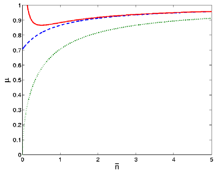
Figure 2: (Color on-line.) Boundaries between different classes of symmetric two-mode Gaussian states. The lower line (green, dotted) is an entanglement boundary given by Eq. (70): states above the line are entangled. The central (blue, dashed) line is a steerability (lower) boundary based on Eq. (77) for the EPR paradox: states above this line are steerable. The upper line (red, full) is a second steerability (lower) boundary based on a generalisation of the entanglement criterion of Duan et al. (Duan2000, ) and Simon (Simon2000, ): states above this line are steerable.

As discussed in Sec. IV, the generalization of Duan et al. and Simon’s entanglement criterion to EPR-steering is given by inequality (59). For states of the form of Eq. (69), the relevant criterion becomes, using the optimal scale factors $g_{x}=-1$ and $g_{p}=1$,

$$\Delta^{2}(x^{A}-x^{B})+\Delta^{2}(p^{A}+p^{B})\geq 2.$$ (72)

For the two-mode symmetric states we find

$$\Delta^{2}(x^{A}-x^{B})=\Delta^{2}(p^{A}+p^{B})=2\gamma-2\delta.$$ (73)

Substituting into (72) and rearranging we find that

$$\mu>\frac{1+4\bar{n}}{4\sqrt{\bar{n}(1+\bar{n})}}$$ (74)

indicates EPR-steering. This condition is plotted in Fig. 2, where states above the line are steerable. For this particular state the additive convex criterion (72) and the corresponding multiplicative criterion

$$\Delta^{2}(x^{A}-x^{B})\Delta^{2}(p^{A}+p^{B})\geq 1,$$ (75)

derived from (37), give the same results, since both variances are identical in this case.

For comparison, recall the EPR-Reid criterion, (38), which tells us that the violation of

$$\Delta_{\mathrm{inf}}x^{B}\Delta_{\mathrm{inf}}p^{B}\geq 1$$ (76)

indicates EPR-steering. Evaluating the left hand side of (76) for two-mode symmetric Gaussian states, using the optimal inference variances $\Delta_{\mathrm{min}}x^{B}$ as defined in Eq. (26), we thus obtain

$$\mu>\sqrt{\frac{1+2\bar{n}}{2(1+\bar{n})}}$$ (77)

as a condition indicating the demonstration of EPR-steering. Also in this case inequality (76) detects EPR-steering just as well as the analogous additive criterion (53), since both inference variances for $x^{B}$ and $p^{B}$ have the same value. In Fig. 2 we see that (76) provides a lower bound on steerability than that provided by (72) (although for $\bar{n}\gg 1$ the two bounds become arbitrarily close). This is not surprising when one remembers, as discussed in Sec. IV.2, that the optimal conditional variances (76) are lower bounds for the linear-estimate inference of the form $\Delta^{2}(g_{x}x^{A}+x^{B})$. In other words, as pointed out in Sec. IV, the EPR criterion is a more sensitive witness to EPR-steering than inequality (72), derived as the steerability generalisation of the entanglement criterion of Duan et al. and Simon.

V.2 Discrete variables

To illustrate the use of EPR-steering criteria in the discrete variable case we will make use of the Werner states (Werner1989, ). For the case of a two-dimensional subsystems, these are a natural mixed-state generalization of the singlet state considered by Bohm, and can be written as follows

$$\rho_{W}=\mu|\psi_{S}\rangle\langle\psi_{S}|+(1-\mu)\frac{\mathbf{I}}{4},$$ (78)

where $|\psi_{S}\rangle=\frac{1}{\sqrt{2}}(|\frac{1}{2}\rangle|-\frac{1}{2}\rangle-|-\frac{1}{2}\rangle|\frac{1}{2}\rangle)$, $\mathbf{I}$ is the identity over both subsystems, and $\mu$ is a mixing parameter that can take values $\mu\leq 1$, with $\mu=0$ again corresponding to a product state (Wiseman2007, ).

It was shown in Ref. (Wiseman2007, ) that the Werner state is steerable in theory with an infinite number of measurements whenever $\mu>1/2$. In order to demonstrate EPR-steering in a realistic experimental setup it is sufficient to instead test a suitable EPR-steering criterion.

We will first evaluate the criterion given by inequality (39). Calculation shows that for the Werner state (78),

$$\Delta_{\mathrm{inf}}^{2}J_{z}^{B}=\frac{1}{4}(1-\mu^{2})$$

and

$$|\langle J_{z}^{B}\rangle|_{\mathrm{inf}}=\frac{\mu}{2}.$$

The Werner state is rotationally symmetric, and thus $\Delta_{\mathrm{inf}}J_{x}^{B}=\Delta_{\mathrm{inf}}J_{y}^{B}=\Delta_{\mathrm{inf}}^{2}J_{z}^{B}$. We therefore find that inequality (39) will be violated (demonstrating EPR-steering) for $\mu>(\sqrt{5}-1)/2\approx 0.62$. This inequality cannot therefore detect all steerable states.

For inequality (57) we make the substitution (as explained below Eq. (57)) $\langle N^{B}\rangle/2=j=1/2$, and with the values for $\Delta_{\mathrm{inf}}^{2}J_{z}^{B}$ a simple calculation reveals violation whenever $\mu>1/\sqrt{3}\approx 0.58$, This inequality, more symmetric between the different measurements, thus detects more steerable states (within the class of Werner states) than the less symmetric (39).

We now proceed to evaluating the linear inequalities (64) and (66). The expectation value of the products of observables required for those inequalities, given the Werner state, is

$$\langle J_{i}^{A}J_{i}^{B}\rangle=-\frac{\mu}{4},$$

where again by symmetry those expectation values are the same for all $i\in\{x,y,z\}$. Substituting in (64) we obtain a violation for $\mu>1/\sqrt{2}\approx 0.71$ and in (66), violation for $\mu>1/\sqrt{3}\approx 0.58$. The first inequality, with only two measurements per site, performs worse (detects less steerable Werner states) than (39), but the second, with three measurements, detects a larger range. Note that the range of states for which violation is predicted using (57) is the same as that detected with (66). The latter, however, offers the advantage of being simpler to measure and calculate.

VI Conclusion

We have developed a general theory of EPR-steering criteria. These criteria are the experimental consequences of a LHS model for one party (Bob), just as Bell inequalities are the experimental consequence of a LHV model and entanglement criteria are consequences of a quantum separable model. The essential ingredients in the derivation of the criteria are the convexity of the set of correlations that allow a LHS model and (generalized) uncertainty relations which define bounds on how Bob’s outcomes can be described by quantum states.

Analysing the different forms of nonlocality, we see that they differ only in how they treat the states of Alice and/or Bob, but they are all convex combinations of separable probability distributions. Some of the criteria derived here were therefore similar to known entanglement criteria, but with a more restrictive bound due to the fact that Alice’s subsystem is treated as an arbitrary hidden-variable state. However others, in particular the linear EPR-steering criteria, are entirely new. These criteria open the possibility to new experimental demonstrations of the EPR-steering phenomenon, with close links to topics in quantum information including entanglement witnesses and quantum cryptography.

- [1] A. Einstein, B. Podolsky, and N. Rosen. Can quantum-mechanical description of physical reality be considered complete? Physical Review, 47:777, 1935.
- [2] J. S. Bell. Introduction to the hidden-variable question. In Foundations of Quantum Mechanics, page 171, New York, 1971. Academic Press.
- [3] M. D. Reid. Demonstration of the Einstein-Podolsky-Rosen paradox using nondegenerate parametric amplification. Physical Review A, 40(2):913–923, 1989.
- [4] H. M. Wiseman. From Einstein’s theorem to Bell’s theorem: a history of quantum non-locality. Contemporary Physics, 47(2):79–88, 2006.
- [5] Vlatko Vedral. Introduction to Quantum Information Science. Oxford University Press, New York, 2006.
- [6] E. Schrodinger. Discussion of probability relations between separated systems. Proc. Cambridge Philos. Soc., 31:555, 1935.
- [7] J. S. Bell. On the Einstein-Podolsky-Rosen paradox. Physics, 1:195, 1964.
- [8] D. Bohm. Quantum Theory, chapter 22. Prentice Hall, Englewood Cliffs, N.J., 1951.
- [9] E. G. Cavalcanti and M. D. Reid. Uncertainty relations for the realization of macroscopic quantum superpositions and EPR paradoxes. Journal of Modern Optics, 54:2373, 2007.
- [10] E. G. Cavalcanti, P. D. Drummond, H. A. Bachor, and M. D. Reid. Unambiguous signatures of entanglement and Bohm’s spin EPR paradox. Optics Express, 17(21):18693–702, 2009. arxiv:0711.3798v1.
- [11] H. M. Wiseman, S. J. Jones, and A. C. Doherty. Steering, entanglement, nonlocality, and the einstein-podolsky-rosen paradox. Physical Review Letters, 98(14):140402, 2007.
- [12] E. Schrödinger. Die gegenwärtige situation in der quantenmechanick. Naturwissenschaften, 23:807, 1935.
- [13] L. M. Duan, G. Giedke, J. I. Cirac, and P. Zoller. Inseparability criterion for continuous variable systems. Physical Review Letters, 84(12):2722–2725, 2000.
- [14] R. Simon. Peres-Horodecki separability criterion for continuous variable systems. Physical Review Letters, 84:2726, 2000.
- [15] H. F. Hofmann and S. Takeuchi. Violation of local uncertainty relations as a signature of entanglement. Physical Review A, 68(3):032103, 2003.
- [16] O. Guhne. Characterizing entanglement via uncertainty relations. Physical Review Letters, 92(11):117903, 2004.
- [17] J. F. Clauser, M. A. Horne, A. Shimony, and R. A. Holt. Proposed experiment to test local hidden-variable theories. Physical Review Letters, 23(15):880, 1969.
- [18] N. D. Mermin. Quantum-mechanics vs local realism near the classical limit: a Bell inequality for spin-s. Physical Review D, 22(2):356–361, 1980.
- [19] A. Fine. Hidden-variables, joint probability, and the Bell inequalities. Physical Review Letters, 48(5):291–295, 1982.
- [20] I. Pitowsky. Quantum Probability - Quantum Logic, volume 321 of Lecture Notes in Physics. Springer-Verlag, 1989.
- [21] M. Ardehali. Bell inequalities with a magnitude of violation that grows exponentially with the number of particles. Physical Review A, 46(9):5375–5378, 1992.
- [22] A. V. Belinskii and D. N. Klyshko. Iinterference of light and Bell’s theorem. Physics-Uspekhi, 36:653, 1993.
- [23] A. Peres. All the Bell inequalities. Foundations of Physics, 29(4):589–614, 1999.
- [24] R. F. Werner and M. M. Wolf. All-multipartite Bell-correlation inequalities for two dichotomic observables per site. Physical Review A, 64(3):032112, 2001.
- [25] D. Collins, N. Gisin, N. Linden, S. Massar, and S. Popescu. Bell inequalities for arbitrarily high-dimensional systems. Physical Review Letters, 88(4):040404, 2002.
- [26] M. Zukowski and C. Brukner. Bell’s theorem for general n-qubit states. Physical Review Letters, 88(21):210401, 2002.
- [27] E. G. Cavalcanti, C. J. Foster, M. D. Reid, and P. D. Drummond. Bell inequalities for continuous-variable correlations. Physical Review Letters, 99:210405, 2007.
- [28] S. J. Jones, H. M. Wiseman, and A. C. Doherty. Entanglement, Einstein-Podolsky-Rosen correlations, Bell nonlocality, and steering. Physical Review A, 76:052116, 2007.
- [29] G. Brassard and A. A. Méthot. Can quantum-mechanical description of physical reality be considered incomplete? International Journal of Quantum Information, 4(1):45–54, 2006.
- [30] E. Schrodinger. Probability relations between separated systems. Proc. Cambridge Philos. Soc., 32:446, 1936.
- [31] N. Gisin. Bell inequality holds for all non-product states. Physics Letters A, 154(5-6):201–202, 1991.
- [32] David Bohm. A suggested interpretation of the quantum theory in terms of "hidden" variables. i. Physical Review, 85:166 – 179, 1952.
- [33] David Bohm. A suggested interpretation of the quantum theory in terms of "hidden" variables. ii. Physical Review, 85:180 – 193, 1952.
- [34] E. Bleuler and H. L. Bradt. Correlation between the states of polarization of the two quanta of annihilation radiation. Physical Review, 73:1398, 1948.
- [35] C. S. Wu and I. Shaknov. The angular correlation of scattered annihilation radiation. Physical Review, 77(1):136–136, 1950.
- [36] Carl A. Kocher and Eugene D. Commins. Polarization correlation of photons emitted in an atomic cascade. Phys. Rev. Lett., 18(15):575–577, 1967.
- [37] W. H. Furry. Note on the quantum-mechanical theory of measurement. Physical Review, 49(5):393–399, 1936.
- [38] M. D. Reid, P. D. Drummond, W. P. Bowen, E. G. Cavalcanti, P. K. Lam, H. A. Bachor, U. L. Andersen, and G. Leuchs. Colloquium: The Einstein-Podolsky-Rosen paradox: From concepts to applications. arXiv:0806.0270, Rev. Mod. Phys., in print, 2009.
- [39] Z. Y. Ou, S. F. Pereira, H. J. Kimble, and K. C. Peng. Realization of the Einstein-Podolsky-Rosen paradox for continuous-variables. Physical Review Letters, 68(25):3663–3666, 1992.
- [40] Y. Zhang, H. Wang, X. Y. Li, J. T. Jing, C. D. Xie, and K. C. Peng. Experimental generation of bright two-mode quadrature squeezed light from a narrow-band nondegenerate optical parametric amplifier. Physical Review A, 62(2):023813, 2000.
- [41] C. Silberhorn, P. K. Lam, O. Weiss, F. Konig, N. Korolkova, and G. Leuchs. Generation of continuous variable Einstein-Podolsky-Rosen entanglement via the Kerr nonlinearity in an optical fiber. Physical Review Letters, 86(19):4267–4270, 2001.
- [42] C. Schori, J. L. Sorensen, and E. S. Polzik. Narrow-band frequency tunable light source of continuous quadrature entanglement. Physical Review A, 66:033802, 2002.
- [43] W. P. Bowen, R. Schnabel, P. K. Lam, and T. C. Ralph. Experimental investigation of criteria for continuous variable entanglement. Physical Review Letters, 90(4):043601, 2003.
- [44] J. C. Howell, R. S. Bennink, S. J. Bentley, and R. W. Boyd. Realization of the Einstein-Podolsky-Rosen paradox using momentum- and position-entangled photons from spontaneous parametric down conversion. Physical Review Letters, 92(21):210403, 2004.
- [45] J. S. Bell. Speakable and Unspeakable in Quantum Mechanics. Cambridge University Press, Cambridge, 1987.
- [46] E. G. Cavalcanti and H. M. Wiseman. to be published.
- [47] A. Einstein. Letter to born, 3 march 1947. In M. Born, editor, The Einstein-Born Letters, page 158. Macmillan, London, 1971.
- [48] C. Cohen-Tannoudji, B. Diu, and F. Lalöe. Quantum Mechanics, volume 1. Wiley Interscience, 1977.
- [49] C. W. Helstrom. Quantum Detection and Estimation Theory, volume 123 of Mathematics in Science and Engineering. Academic Press, New York, 1976.
- [50] W. P. Bowen, R. Schnabel, P. K Lam, and T. C. Ralph. Experimental characterization of continuous-variable entanglement. Phys. Rev. A, 69(1):012304, 2004.
- [51] R. F. Werner. Quantum states with Einstein-Podolsky-Rosen correlations admitting a hidden-variable model. Physical Review A, 40(8):4277–4281, 1989.