Two-dimensional boson-fermion mixtures

Abstract

Using mean-field theory, we study the equilibrium properties of boson-fermion mixtures confined in a harmonic pancake-shaped trap at zero temperature. When the modulus of the $s$-wave scattering lengths are comparable to the mixture thickness, two-dimensional scattering events introduce a logarithmic dependence on density in the coupling constants, greatly modifying the density profiles themselves. We show that for the case of a negative boson-fermion three-dimensional $s$-wave scattering length, the dimensional crossover stabilizes the mixture against collapse and drives it towards spatial demixing.

I Introduction

Fermionic atomic gases were brought together with bosonic atoms to quantum degeneracy in several alkali atom mixtures, such as ⁷Li-⁶Li Truscott2001a ; Schreck2001a , ²³Na-⁶Li Hadzibabic2002a , ⁸⁷Rb-⁴⁰K Goldwin2002a ; Roati2002a ; Modugno2002a , and very recently in a mixed gas of ytterbium (Yb) isotopes, ¹⁷⁴Yb-¹⁷³Yb Fukuhara2009 . The boson-fermion (BF) coupling strongly affects the equilibrium properties of the mixture and can drive quantum phase transitions, as collapse Modugno2002a in the presence of attractive BF interaction, or spatial demixing as recently observed in the context of three-dimensional (3D) atomic fermion - molecular boson mixtures Partridge2006a ; Shin2006a , where the strong interspecies repulsion leads to phase separation.

Such mixtures can be realized from an imbalanced two-component Fermi gas (⁴⁰K-⁴⁰K or ⁶Li-⁶Li mixtures) where all minority fermions become bound as bosons and form a Bose-Einstein condensate (BEC). Though imbalanced Fermi gases allowed to observe spatial phase separation between bosonic dimers and fermions, the advantage of a two atomic species BF mixture is that boson-boson (BB) and BF interactions can be driven independently and that one can access attractive BF interactions Ospelkaus2006a ; Zaccanti2006a .

The structure and the stability of trapped BF mixtures were studied in 3D by using the Thomas-Fermi approximation for the bosonic component Molmer1998 ; Akdeniz2002 and by using a modified Gross-Pitaevskii (GP) equation for the bosons which self-consistently includes the mean-field interaction generated by the fermionic cloud Roth2002 ; pelster . Effects of the geometry induced by the trap deformation were studied in the Thomas-Fermi regime in a quasi-3D limit, i.e. when collisions can be still considered as three-dimensional Akdeniz2004 . Such a simple model predicts, in a pancake-shaped trap, that the stability of the mixture depends only on the scattering length and the transverse width of the cloud. One should expect, in a true dimensional crossover, namely including dimensional effects in scattering events, that the mixture stability depends critically on the energy, and thus on the number of particles.

The dimensional crossover from a 3D to a 2D trapped mixture may be studied in the experiments by flattening magnetic or dipolar confinements Gorlitz2001 , or by trapping atoms in specially designed pancake potentials, as rotating traps Schweikhard2004 , gravito-optical surface traps Rychtarik2004 , rf-induced two-dimensional traps Colombe2004 or in one-dimensional lattices Stock2005 where a 3D gas can be split in several independent disks.

In the limit where scattering events are bi-dimensional, it is well known that a hard-core boson gas shows very different features from its 3D counterpart. In 3D, particle interactions can be described by the zero-momentum and zero-energy limit of $T$-matrix, leading to a constant coupling parameter. In 2D, $T$-matrix vanishes at low momentum and energy Schick1971 ; Popov1966 and the first-order contribution to the coupling is obtained by taking into account the many-body shift in the effective collision energy of two-condensate atoms alkhawaja ; lee2 . This leads to an energy dependent coupling parameter that greatly affects the equilibrium and the dynamical properties of the gas Tanatar2002 ; Hosten2003 .

In this paper we study the equilibrium properties of a mixture of condensed bosons and spin-polarized fermions, through the dimensional crossover from three to two dimensions, by following the procedure outlined by Roth Roth2002 for the 3D mixture. We neglect fermion-fermion interactions and we include BF $s$-wave interaction self-consistently in a suitably modified GP equation for the bosons. For the case of BF repulsive interaction, the increasing anisotropy softens the repulsion, and a quasi-3D spatially demixed mixture is mixed in quasi-2D. For the case of BF attractive interactions, the dimensional crossover acts as a Feshbach resonance and induce repulsive interactions, so that a Q3D mixture near collapse can be driven towards spatial demixing in Q2D. In the strictly 2D regime the results depend on the model one assumes for the bi-dimensional scattering lengths.

The paper is organized as follows. In Sec. II we introduce the theoretical mean-field model for the description of ground-state density profiles of the BF mixture. The models for the coupling through the dimensional crossover are outlined in Sec. III. The density profiles obtained for a ⁶Li-⁷Li and a ⁴⁰K-⁸⁷Rb mixtures are shown in Sec. IV. Section V offers a summary and some concluding remarks.

II Mean-field model for the density profiles

We consider a BF mixture in a 2D geometry, with respective particle numbers $N_{B}$ and $N_{F}$, confined in harmonic trap potentials $V_{B,F}=\frac{1}{2}m_{B,F}\omega_{B,F}^{2}r^{2}$. Here $m_{B,F}$ is boson (fermion) mass and $\omega_{B,F}$ is the radial trap frequency as seen by boson or fermion species. Within the mean-field approach the total energy functional at $T=0$ is written as

$$\begin{split}E[\psi_{B},\psi_{F}]&=\int\,d^{2}r\left\{\frac{\hbar^{2}}{2m_{B}}|\nabla\psi_{B}|^{2}+V_{B}(r)|\psi_{B}|^{2}+\frac{1}{2}g_{BB}|\psi_{B}|^{4}\right\}\\ &\quad+\int\,d^{2}r\left\{T_{F}+V_{F}(r)|\psi_{F}|^{2}\right\}+\int\,d^{2}r\,g_{BF}|\psi_{B}|^{2}|\psi_{F}|^{2},\end{split}$$ (1)

where $\psi_{B,F}$ is the ground-state wave function of bosons and fermions, respectively. In the above boson species are in the condensed state and fermion species is assumed to be spin-polarized and its kinetic energy is written within the Thomas-Fermi-Weizsacker approximation as zaremba ; jezek

$$T_{F}=\frac{\hbar^{2}}{m_{F}}\left(\pi n_{F}^{2}+\frac{\lambda_{W}}{8}\frac{|\nabla n_{F}|^{2}}{n_{F}}\right)\,,$$ (2)

where $n_{F}=|\psi_{F}|^{2}$ is the fermion density and the Weizsacker constant is $\lambda_{W}=1/4$. Normalization conditions for $N_{B}$ bosons and $N_{F}$ fermions read $N_{B}=\int d^{2}r|\psi_{B}|^{2}$ and $N_{F}=\int d^{2}r|\psi_{F}|^{2}$. The interaction couplings between the bosons and between bosons and fermions are denoted by $g_{BB}$ and $g_{BF}$, respectively. One notable difference between the form of the energy functional given above and that in 3D, is that the BB and BF interaction strengths are in general density dependent in contrast to the situation in 3D. More specifically, in 3D the interaction strengths are proportional to the scattering lengths $a_{BB}$ and $a_{BF}$ whereas in 2D as we shall explain below they depend on the density or equivalently the chemical potential. The Euler-Lagrange equations for the mixture read jezek

$$\left\{-\frac{\hbar^{2}}{2m_{B}}\nabla^{2}+V_{B}+g_{BB}|\psi_{B}|^{2}+g_{BF}|\psi_{F}|^{2}-\mu_{B}\right\}\psi_{B}=0\,,$$ (3)

and

$$\left\{-\frac{\hbar^{2}}{2m_{F}}\lambda_{W}\nabla^{2}+V_{F}+\frac{\hbar^{2}}{m_{F}}2\pi|\psi_{F}|^{2}+g_{BF}|\psi_{B}|^{2}-\mu_{F}\right\}\psi_{F}=0\,,$$ (4)

in which we have introduced the chemical potentials $\mu_{B,F}$ for bosons and fermions. The above equations of motion are obtained by functional differentiation from $E[\psi_{B},\psi_{F}]$ neglecting the higher-order terms involving $\delta g/\delta\psi_{B,F}$ which is valid in the dilute gas limit $n_{B}a_{BB}^{2}\ll 1$ and $n_{F}a_{BF}^{2}\ll 1$. The dilute gas conditions above further maintain that beyond mean-field corrections are not called for. They can become notable when $a_{BB},\,a_{BF}$ and/or $N_{B},\,N_{F}$ are large for fixed trap frequencies. For the systems under consideration we have chosen the parameters appropriately and verified by numerical calculations so that $n_{B}a_{BB}^{2},\,n_{F}a_{BF}^{2}\ll 1$. Therefore, in the examples we shall discuss subsequently, the beyond mean-field terms in the energy functional are not important.

It should also be noted that the existence of BEC in 2D needs to be treated carefully. Initial attempts have concluded that no BEC could occur in 2D trapped gases but recent considerations within the Hartree-Fock-Bogoliubov approximation, gies_PRA the density dependent interaction strength bhaduri and numerical simulations markus have established firmly the occurrence of BEC for such systems. Thus, our assumption of a 2D condensate at $T=0$ is justified.

III 2D Interaction Models

In cold atom experiments a 2D geometry is obtained by trapping the atoms in a highly anisotropic trap where the axial confinement is very tight, so that the axial potential is on the same order or larger than the chemical potentials of the two components. Within this condition, the axial widths are on the order of the oscillator lengths for the axial direction $a_{jz}=\sqrt{\hbar/m_{j}\omega_{jz}}$, $\omega_{jz}$ being the axial trap frequency for bosons ($j=B$) and for fermions ($j=F$). For simplicity, here and in the following we assume that $a_{Bz}=a_{Fz}=a_{z}$.

The value of $a_{z}$ with respect to the modulus of the 3D scattering lengths, determines whether the scattering events occur in 3D or in 2D, and thus suggests how to calculate the many-body interaction potentials.

The interaction couplings $g_{BB}$ and $g_{BF}$ are determined microscopically from the effective interaction potentials (two-body scattering amplitude, $T$-matrix, etc.) in the limit of low energy and momenta. In the case of a 3D system, the scattering amplitude and $g_{BB}$ and $g_{BF}$ are constants determined by the $s$-wave scattering lengths $a_{BB}$ and $a_{BF}$. In 2D the scattering theory approaches give rise to a logarithmic dependence Schick1971 ; Popov1966 . Starting from a 3D system and increasing the anisotropy (by increasing the trap frequencies in the axial direction) the geometry flattens to take a pancake shape and eventually a genuine 2D system is obtained. In the following we identify different scattering regimes depending on the relation between the axial confinement length and scattering lengths and provide expressions for the interaction couplings in these regimes.

III.1 Quasi-3D scattering

In this regime, the axial oscillator length $a_{z}$ of the mixture is assumed to be larger than the modulus of $a_{BB}$ and $a_{BF}$, the $s$-wave scattering lengths for BB and BF interactions, respectively.

The effective BB interaction strength can be obtained by multiplying the 3D value of the coupling $g_{BB}^{3D}=4\pi\hbar^{2}a/m_{B}$ with a factor $|\phi(0)|^{2}=1/\sqrt{2\pi}a_{z}$, $\phi(z)$ being the axial wavefunction. This is obtained by assuming that the motion in the $z$-direction is frozen in the ground state of the harmonic potential with trapping frequency $\omega_{jz}$ and integrating the 3D GP equation over $z$ (after multiplying with $\phi^{*}(z)$ in the spirit of taking an expectation value. The chemical potential $\mu$ gets shifted by $\hbar\omega_{jz}/2$). Assuming that the profile for fermions to also be Gaussian in the $z$-direction, we apply the same idea to the BF interaction $g_{BF}^{3D}=2\pi\hbar^{2}a/m_{BF}$, where $m_{BF}$ is the reduced mass. Thus, we obtain

$$g_{BB}=\frac{2\sqrt{2\pi}\hbar^{2}}{m_{B}}\frac{a_{BB}}{a_{z}}\,,\,\,\,\hbox{and}\,\,\,g_{BF}=\frac{\sqrt{2\pi}\hbar^{2}}{m_{BF}}\frac{a_{BF}}{a_{z}},$$ (5)

as the effective interaction couplings in the quasi-3D scattering regime.

III.2 Strictly-2D scattering

This regime corresponds to the limit $a_{z}\ll|a_{BB}|,|a_{BF}|$. The coupling parameter we use is from a $T$-matrix calculation alkhawaja ; lee2 ; lee which takes into account the many-body shift in the effective collision energy of two condensate atoms and it becomes a self-consistent problem. Since $a_{z}<|a_{BB}|$, $|a_{BF}|$ the calculation is purely 2D, and the interaction strengths do not depend on the parameters in the $z$-direction. Al Khawaja et al. alkhawaja argue that when two condensate atoms collide at zero momentum they both require an energy $\mu_{B}$ to be excited from the condensate and thus the many-body coupling is given by evaluating at $-2\mu_{B}$ the two-body $T$-matrix ($T_{2b}$) setting $g_{BB}=\langle 0|T_{2b}(-2\mu_{B})|0\rangle$. On the other hand, Lee et al. lee calculate $T_{2b}$ at $-\mu_{B}$ arguing that this result includes the effect of quasiparticle energy spectrum of the intermediate states in the collision. Gies et al. gies claim that Al Khawaja et al. alkhawaja argument that the excitation of a single condensate atom is associated with an energy of $-\mu_{B}$ includes on the mean-field energy of initial and final states and neglects the other many-body effects on the collision which presumably are included in the result $g_{BB}=\langle 0|T_{2b}(-\mu_{B})|0\rangle$. With this proviso we take

$$g_{BB}=\frac{-4\pi\hbar^{2}}{m_{B}}\frac{1}{\ln{(\mu_{B}m_{B}a_{BB}^{2}/4\hbar^{2})}}$$ (6)

and similarly,

$$g_{BF}=\frac{-2\pi\hbar^{2}}{m_{BF}}\frac{1}{\ln{((\mu_{B}+\mu_{F})m_{BF}a_{BF}^{2}/4\hbar^{2}]}}$$ (7)

where the scattering lengths $a_{BB}=a_{BB}^{2D}$ and $a_{BF}=a_{BF}^{2D}$ are in principle 2D scattering lengths. Our choice for the 2D scattering lengths will be discussed in Sec. IV. In the case of BF interaction strength we used the reduced mass $m_{BF}$ and made the replacement $\mu\rightarrow(\mu_{B}+\mu_{F})/2$. Similar considerations to write down the BF $T$-matrix were also made by Mur-Petit et al. murpetit .

In this regime the interaction parameters must be determined self-consistently. The way the equations are written above suggests to solve for wave functions for given values of $g_{BB}$ and $g_{BF}$, then calculate chemical potentials

$$\mu_{B}=\frac{1}{N_{B}}\int\,d^{2}r\left\{\frac{\hbar^{2}}{2m_{B}}|\nabla\psi_{B}|^{2}+\frac{1}{2}m_{B}\omega_{B}^{2}r^{2}|\psi_{B}|^{2}+g_{BB}|\psi_{B}|^{4}+g_{BF}|\psi_{F}|^{2}|\psi_{B}|^{2}\right\}$$ (8)

and

$$\mu_{F}=\frac{1}{N_{F}}\int\,d^{2}r\left\{\frac{\hbar^{2}}{2m_{F}}\lambda_{W}|\nabla\psi_{F}|^{2}+\frac{1}{2}m_{F}\omega_{F}^{2}r^{2}|\psi_{F}|^{2}+\frac{\hbar^{2}}{m_{F}}2\pi|\psi_{F}|^{4}+g_{BF}|\psi_{F}|^{2}|\psi_{B}|^{2}\right\}$$ (9)

and check whether the expressions for $g_{BB}$ and $g_{BF}$ are satisfied. To follow common practice we start with initial chemical potentials, calculate $g$’s and then calculate chemical potentials using the obtained wave functions and require self-consistency. Note that in this regime the results do not depend on the value of $\omega_{jz}$, i.e. on the value of the anisotropy parameter $\lambda=\omega_{Bz}/\omega_{B}$.

III.3 Quasi-2D scattering

When $a_{z}\gtrsim|a_{BB}|,|a_{BF}|$ collisions are bi-dimensional but influenced by the $z$-direction. In this regime, which is in between the previous cases, the 2D scattering length can be expressed in terms of the 3D scattering length Petrov2001 . Substituting

$$a^{2D}_{ij}=2\sqrt{2}\sqrt{\frac{\pi}{B}}a_{z}e^{-\sqrt{\pi/2}\frac{a_{z}}{a^{3D}_{ij}}}$$ (10)

in the coupling strength expressions for strictly 2D regime with $B\approx 0.915$, the coupling strengths now become lee

$$g_{BB}=\frac{\frac{2\sqrt{2\pi}\hbar^{2}}{m_{B}}\frac{a_{BB}}{a_{z}}}{1+\frac{1}{\sqrt{2\pi}}\frac{a_{BB}}{a_{z}}\ln(B\hbar^{2}/2\pi\mu_{B}m_{B}a_{z}^{2})}$$ (11)

and

$$g_{BF}=\frac{\frac{\sqrt{2\pi}\hbar^{2}}{m_{BF}}\frac{a_{BF}}{a_{z}}}{1+\frac{1}{\sqrt{2\pi}}\frac{a_{BF}}{a_{z}}\ln(B\hbar^{2}/2\pi(\mu_{B}+\mu_{F})m_{BF}a_{z}^{2})}.$$ (12)

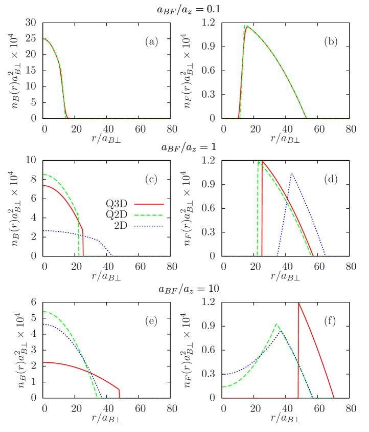
Figure 1: (Color online) Boson and fermion density profiles for ⁶Li-⁷Li mixture with $N_{B}=10^{6}$ and $N_{F}=5\times 10^{5}$, radial trapping frequencies $\omega_{B}/2\pi=4000\,Hz$, $\omega_{F}/2\pi=3520\,Hz$ and scattering lengths $a_{BB}=5.1\,a_{0}$, $a_{BF}=38\,a_{0}$ where $a_{0}$ is the Bohr radius. The length unit is the radial harmonic oscillator length for bosons $a_{B\perp}=\sqrt{\hbar/m_{B}\omega_{B}}$. The density given is in units of $10^{-4}a_{B\perp}^{-2}$ and is normalized to unity. The three regimes $a_{BF}/a_{z}=0.1,\,1,\,10$ correspond to values of the asymmetry parameter $\lambda\approx 10^{3},\,10^{5}$, and $10^{7}$, respectively.

IV Results and Discussion

We first consider a lithium mixture with particle numbers $N_{B}=10^{6}$ and $N_{F}=5\times 10^{5}$, and radial trapping frequencies $\omega_{B}/2\pi=4000$ Hz and $\omega_{F}/2\pi=3520$ Hz. The BB and BF scattering lengths are taken as $a_{BB}=5.1\,a_{0}$ and $a_{BF}=38\,a_{0}$, respectively, in which $a_{0}$ is the Bohr radius.

In Fig. 1 we show the density distributions $n_{B}(r)$ and $n_{F}(r)$ of bosonic and fermionic components in the three scattering regimes: the quasi-3D, where the coupling is given by Eq. (5), the quasi-2D, where the coupling is given in Eqs. (11) and (12), and the strictly 2D, where we use the coupling given in Eqs. (6) and (7) and where we set the bi-dimensional scattering lengths equal to $a^{2D}_{ij}$ (Eq. (10)) evaluated in the limit of vanishing $a_{z}/a^{3D}_{ij}$. This choice assures the strictly 2D model to be the limiting case of the Q2D, that depicts the crossover behavior.

When $a_{BF}/a_{z}=0.1$ (top panel) the mixture has 3D character in terms of collisions even though the geometrical confinement ($\lambda=10^{3}$) renders the system 2D kinematically. The calculated chemical potentials $\mu_{B}/\hbar\omega_{Bz}$ and $\mu_{F}/\hbar\omega_{Fz}$ being less than unity also confirms that the system is geometrically 2D. In this regime the density distributions for quasi-3D and quasi-2D models look very similar. The boson and fermion components occupy the inner and outer parts of the disk giving a segregated phase for the chosen parameters. The 2D model is evidently inapplicable in this regime because $a_{BF}/a_{z}<1$.

In the middle panels of Fig. 1 we show density profiles for the same mixture with $a_{BF}/a_{z}=1$ for an anisotropy parameter $\lambda=10^{5}$. This corresponds to a completely frozen motion in the $z$-direction and to the crossover in the scattering properties from 3D to 2D. Figures 1(c) and 1(d) reveal that the density profiles in the three models are very similar, except for the fact that the 2D model predicts a larger spatial extension of the density profiles.

Finally, in the bottom panel of Fig. 1 we consider $a_{BF}/a_{z}=10$ with $\lambda=10^{7}$. $a_{z}$ being smaller than in the previous case, the bi-dimensional scattering lengths are smaller and both the 2D and Q2D models predict a mixed phase even in the center of the trap, while the Q3D curves still show phase separation. For this anisotropy parameter, the scattering events should be truly 2D and our corresponding model should yield the most accurate density profiles. Evidently the Q3D model is not yet valid, but we plot it just to compare the predictions of the different models.

We now turn our attention to ⁴⁰K-⁸⁷Rb mixture having an attractive BF scattering length. We consider a system with particle numbers $N_{B}=10^{6}$ and $N_{F}=5\times 10^{5}$, and radial trapping frequencies $\omega_{B}/2\pi=257$ Hz and $\omega_{F}/2\pi=378$ Hz. The BB and BF scattering lengths are taken as $a_{BB}=110\,a_{0}$ and $a_{BF}=-284\,a_{0}$, respectively ospelkaus . For attractive interactions, the effective 2D BF scattering length is positive [see Eq. (10)], namely the dimensional crossover induces effective repulsive interactions murpetit , as already predicted in a condensate with attractive boson-boson interaction Petrov2001 . Thus, the strictly 2D couplings (Refs. lee ; alkhawaja ; gies ; murpetit ) refer to hard-core collisions Schick1971 .

Figure 2 illustrates the density profiles $n_{B}(r)$ and $n_{F}(r)$ in quasi-3D and 2D scattering regimes, characterized by $a_{BF}/a_{z}=-0.3$ ($\lambda\approx 2\times 10^{2}$) and $a_{BF}/a_{z}=-10$ ($\lambda\approx 2\times 10^{5}$), respectively. In the case $a_{BF}/a_{z}=-0.3$, we observe that the density profiles are similar for quasi-3D and quasi-2D models and show a bump in the center of the fermionic density due to the attractions with the bosons. For $a_{BF}/a_{z}=-10$, the Q2D model approaches the 2D one, the only difference being that the first model predicts complete spatial separation between the bosonic and the fermionic components, while the second predicts a residual mixed phase at the center of the trap.

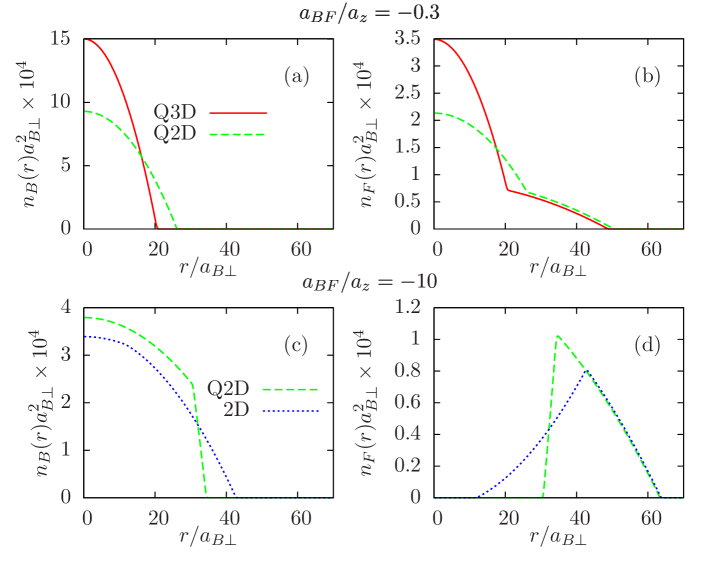
Figure 2: (Color online) Same as in Fig. 1 for a ⁴⁰K-⁸⁷Rb mixture with $N_{B}=10^{6},N_{F}=5\times 10^{5}$. The values of $|a_{BF}|/a_{z}=0.3,\,10$ correspond to $\lambda\approx 2\times 10^{2}$ and $2\times 10^{5}$.

The crossover between the two regimes is shown in Fig. 3. For $\lambda<10^{2}$, the fermionic density is enhanced at the center of the trap because of the presence of the bosons. In this regime the BF coupling term is negative, as shown in Fig. 4. At $\lambda=10^{5}$ the fermions are pushed out of the center of the trap because of the large repulsive BF interaction (see Fig. 4). By increasing further and further the anisotropy, the BF coupling is still positive but decreases and the two components are partially mixed. For $10^{2}<\lambda<10^{5}$ no stable solutions are found.

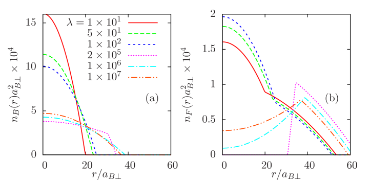
Figure 3: (Color online) Density profiles for the ⁴⁰K-⁸⁷Rb mixture calculated with the Q2D model for various values of $\lambda$. (Same units as in Fig. 1.)

Thus, as shown in Fig. 4, the dimensional crossover plays the role of a Feshbach resonance. Squeezing the trap one may naively expect the gas just collapsing, but the crossover in the scattering geometry changes the nature of the instability from collapse to demixing, and a further squeezing of the trap stabilizes the mixture.

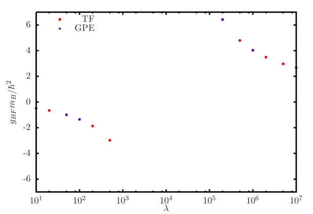
Figure 4: (Color online) Effective BF interaction strength (in dimensionless units) for the ⁴⁰K-⁸⁷Rb mixture within the Q2D model as a function of the anisotropy parameter $\lambda$. Dots refer to the numerical calculation performed in the Thomas-Fermi (TF) approximation, namely neglecting the Laplacian terms in Eqs. (3) and (4), while triangles refer to the full solution of the same equations (GPE).

All curves shown in this sections correspond to densities that fulfill the diluteness conditions $n_{B}a_{BB}^{2}\ll 1$ and $n_{F}a_{BF}^{2}\ll 1$, even at close to the resonance shown in Fig. 4.

V Summary

In summary we have studied the equilibrium properties of a boson-fermion mixture confined in a pancake-shaped trap, in the dimensional crossover from 3D to 2D. The boson-boson and the boson-fermion couplings used are those derived from the two-body $T$-matrix evaluated (i) at zero energy in 3D, (ii) taking into account the discreteness of the spectrum in the axial direction, in the crossover, (iii) taking into account the many-body energy shift in the strictly 2D limit. The density profiles and the couplings have been evaluated self-consistently using suitable modified coupled Gross-Pitaevskii equations for the bosonic and the fermionic wave functions.

For the case of a positive 3D boson-fermion scattering length, the dimensional crossover softens the repulsion, so that the components of a demixed boson-fermion mixture in 3D can mix in the 2D limit. For the case of a negative 3D boson-fermion scattering length, the dimensional crossover is more dramatic and plays the role of a Feshbach resonance. Our study shows that the squeezing of the pancake-shaped trap may drive a strong-attractive unstable mixture towards a stable mixed mixture passing through a demixed phase. This numerical study may be reproduced in the actual experiments with BF mixtures. The goal being to reach a regime where the modulus of the scattering lengths is comparable or greater than the mixture axial size, one may exploit Feschbach resonances to increase the magnitude of the 3D scattering lengths, or one may engineer very flat traps as already done in the context of experiments with a single BEC component.

- (1) A.G. Truscott, K.E. Strecker, W.I. McAlexander, G.B. Partridge and R.G. Hulet, Science 291, 2570 (2001).
- (2) F. Schreck, L. Khaykovich, K.L. Corwin, G. Ferrari, T. Bourdel, J. Cubizolles and C. Salomon, Phys. Rev. Lett. 87, 080403 (2001).
- (3) Z. Hadzibabic, C.A. Stan, K. Dieckmann, S. Gupta, M.W. Zwierlein, A. Görlitz and W. Ketterle, Phys. Rev. Lett. 88, 160401 (2002).
- (4) J. Goldwin, S.B. Papp, B. DeMarco and D.S. Jin, Phys. Rev. A 65, 021402(R) (2002).
- (5) G. Roati, F. Riboli, G. Modugno and M. Inguscio, Phys. Rev. Lett. 89, 150403 (2002).
- (6) G. Modugno, G. Roati, F. Riboli, F. Ferlaino, R.J. Brecha and M. Inguscio, Science 297, 2240 (2002).
- (7) T. Fukuhara, S. Sugawa, Y. Takasu, and Y. Takahashi, Phys. Rev. A 79, 021601(R) (2009).
- (8) G.B. Partridge, W. Li, R.I. Kamar, Y. Liao, and R.G. Hulet, Science 311, 503 (2006).
- (9) Y. Shin, M.W. Zwierlein, C.H. Schunck, A. Schirotzek, W. Ketterle, Phys. Rev. Lett. 97, 030401 (2006).
- (10) S. Ospelkaus, C. Ospelkaus, L. Humbert, K. Sengstock, and K. Bongs, Phys. Rev. Lett. 97, 120403 (2006).
- (11) M. Zaccanti, C. D’Errico, F. Ferlaino, G. Roati, M. Inguscio, and G. Modugno, Phys. Rev. A 74, 041605(R) (2006).
- (12) K. Mølmer, Phys. Rev. Lett. 80, 1804 (1998).
- (13) Z. Akdeniz,P. Vignolo, A. Minguzzi, and M.P. Tosi, J. Phys. B 35, L105 (2002).
- (14) R. Roth, Phys. Rev. A 66, 013614 (2002).
- (15) S. Röthel and A. Pelster, Eur. Phys. J. B 59, 343 (2007).
- (16) Z. Akdeniz, P. Vignolo, and M.P. Tosi, Phys. Lett. A 331, 258 (2004).
- (17) A. Görlitz, J. M. Vogels, A. E. Leanhardt, C. Raman, T. L. Gustavson, J. R. Abo-Shaeer, A. P. Chikkatur, S. Gupta, S. Inouye, T. Rosenband, and W. Ketterle, Phys. Rev. Lett. 87, 130402 (2001).
- (18) V. Schweikhard, I. Coddington, P. Engels, V. P. Mogendorff, and E. A. Cornell, Phys. Rev. Lett. 92, 040404 (2004).
- (19) D. Rychtarik, B. Engeser, H.-C. Nägerl, and R. Grimm, Phys. Rev. Lett. 92, 173003 (2004).
- (20) Y. Colombe, E. Knyazchyan, O. Morizot, B. Mercier, V. Lorent, H. Perrin, Europhys. Lett. 67, 593 (2004).
- (21) S. Stock, Z. Hadzibabic, B. Battelier, M. Cheneau, J. Dalibard, Phys. Rev. Lett. 95, 190403 (2005).
- (22) M. Schick, Phys. Rev. A 3, 1067 (1971).
- (23) V.N. Popov, Functional Integrals in Quantum Field Theory and Statistical Physcis (Reidel, Dordrecht 1983), Chap. 6.
- (24) U. Al Khawaja, J.O. Andersen, N.P. Proukakis, and H.T.C. Stoof, Phys. Rev. A 66, 013615 (2002).
- (25) M.D. Lee, S.A. Morgan, M.J. Davis, and K. Burnett, Phys. Rev. A 65, 043617 (2002).
- (26) B. Tanatar, A. Minguzzi, P. Vignolo, and M.P. Tosi, Phys. Lett. A 302, 131 (2002).
- (27) O. Hosten, P. Vignolo, A. Minguzzi, B. Tanatar and M.P. Tosi, J. Phys. B: At. Mol. Opt. Phys. 36 2455 (2003).
- (28) See for instance, B.P. van Zyl and E. Zaremba, Phys. Rev. B 59, 2079 (1999).
- (29) D.M. Jezek, M. Barranco, M. Guilleumas, R. Mayol, and M. Pi, Phys. Rev. A 70, 043630 (2004); M. E. Tasgin, A. L. Subasi, M.O. Oktel, and B. Tanatar, J. Low Temp. Phys. (2005).
- (30) C. Gies, B.P. van Zyl, S.A. Morgan, and D.A.W. Hutchinson, Phys. Rev. A 69, 023616 (2004).
- (31) B.P. van Zyl, R.K. Bhaduri, and J. Sigetich, J. Phys. B: At. Mol. Opt. Phys. 35, 1251 (2002).
- (32) M. Holzmann and W. Krauth, Phys. Rev. Lett. 100, 190402 (2008).
- (33) M.D. Lee and S.A. Morgan, J. Phys. B: At. Mol. Opt. Phys. 35, 3009 (2002).
- (34) C. Gies, M.D. Lee, and D.A.W. Hutchinson, J. Phys. B: At. Mol. Opt. Phys. 38, 1797 (2005).
- (35) J. Mur-Petit, A. Polls, M. Baldo, and H.-J. Schulze, Phys. Rev. A 69, 023606 (2004); J. Phys. B: At. Mol. Opt. Phys. 37, S165 (2004).
- (36) D.S. Petrov and G.V. Shlyapnikov, Phys. Rev. A, 64, 012706 (2001).
- (37) C. Ospelkaus, S. Ospelkaus, K. Sengstock, and K. Bongs, Phys. Rev. Lett. 96, 020401 (2006).