AzTEC Half Square Degree Survey of the SHADES Fields – I. Maps, Catalogues, and Source Counts

Abstract

We present the first results from the largest deep extragalactic millimetre-wavelength survey undertaken to date. These results are derived from maps covering over 0.7 deg², made at $\lambda=1.1$ mm, using the AzTEC continuum camera mounted on the James Clerk Maxwell Telescope. The maps were made in the two fields originally targeted at $\lambda=850$ $\micron$ with the Submillimetre Common-User Bolometer Array (SCUBA) in the SHADES project, namely the Lockman Hole East (mapped to a depth of 0.9–1.3 mJy rms) and the Subaru XMM Deep Field (mapped to a depth of 1.0–1.7 mJy rms). The wealth of existing and forthcoming deep multi-frequency data in these two fields will allow the bright mm source population revealed by these new wide-area 1.1 mm images to be explored in detail in subsequent papers. Here we present the maps themselves, a catalogue of 114 high-significance sub-millimetre galaxy detections, and a thorough statistical analysis leading to the most robust determination to date of the 1.1 mm source number counts. These new maps, covering an area $\sim 3$ times greater than the SCUBA SHADES maps, currently provide the largest sample of cosmological volumes of the high-redshift Universe in the mm or sub-mm. Through careful comparison, we find that both the COSMOS and GOODS North fields, also imaged with AzTEC, contain an excess of mm sources over the new 1.1 mm source-count baseline established here. In particular, our new AzTEC/SHADES results indicate that very luminous high-redshift dust enshrouded starbursts ($S_{\rm{1.1mm}}>3$ mJy) are 25–50 per cent less common than would have been inferred from these smaller surveys, thus highlighting the potential roles of cosmic variance and clustering in such measurements. We compare number count predictions from recent models of the evolving mm/sub-mm source population to these SMG surveys, which provide important constraints for the ongoing refinement of semi-analytic and hydrodynamical models of galaxy formation, and find that all available models over-predict the number of bright sub-millimetre galaxies found in this survey.

1 Introduction

In the last two decades, surveys in the far-infrared and sub-millimetre have revolutionised our understanding of galaxy evolution in the high-redshift Universe. These surveys, primarily at wavelengths around 850–$\micron$ (e.g. Smail et al., 1997; Hughes et al., 1998; Barger et al., 1998; Scott et al., 2002; Borys et al., 2003; Pope et al., 2006; Coppin et al., 2006; Greve et al., 2009), 1100–$\micron$ (Laurent et al., 2005; Scott et al., 2008; Perera et al., 2008), and 1200–$\micron$ (e.g. Greve et al., 2004; Bertoldi et al., 2007; Greve et al., 2008) have shown that the contribution to the comoving IR energy density from sub-mm bright galaxies (SMGs) increases by approximately three orders of magnitude in going from the local Universe to $z\mathrel{\lower 2.5pt\vbox{\hbox{$>$}\hbox{$\sim$}}}1$, and that $z\mathrel{\lower 2.5pt\vbox{\hbox{$>$}\hbox{$\sim$}}}1$ SMGs are responsible for a significant portion the extragalactic infrared background light (e.g. Scott et al., 2008; Serjeant et al., 2008). Initial followup studies have identified optical counterparts (e.g. Dye et al., 2008; Clements et al., 2008) and measured redshifts (e.g. Chapman et al., 2005; Aretxaga et al., 2007) of many SMGs. Further studies have shown that SMGs harbour very high rates of star formation, often accompanied by significant AGN activity (e.g. Alexander et al., 2005; Kovács et al., 2006; Coppin et al., 2008; Menéndez-Delmestre et al., 2007; Pope et al., 2008) and that at least some are involved in ongoing mergers (Farrah et al., 2002; Chapman et al., 2003), implying that SMGs signpost massive galaxy assembly in the high redshift Universe. Reviews of their properties can be found in Blain et al. (2002) and Lonsdale et al. (2006).

On a fundamental level, SMGs represent the efficient transformation of free baryons into stars and black holes. Recent work has therefore focused on understanding how SMGs relate to the cosmological evolution of the total and baryonic mass density. Evidence suggests that this relationship is complex, with an intricate dependence on variables such as redshift, local environmental richness, and halo merger history. Accordingly, observations must find SMGs across a wide range of environments and redshifts. This has traditionally proven difficult; SMGs are easy to find across wide redshift ranges due to the favourable k-correction at sub-mm wavelengths, but hard to find across wide ranges in environment due to the inability of most sub-mm bolometer arrays to efficiently map large areas of sky. Constraints on SMG number counts have thus been limited by both sample size and cosmic variance, we have found relatively few of the brightest and rarest SMGs, and constraints on SMG clustering – an important tool in relating SMGs to the underlying dark matter distribution – are weak (Blain et al., 2004; van Kampen et al., 2005; Chapman et al., 2009, e.g., see also Farrah et al., 2006; Magliocchetti et al., 2007). As a result, many studies have adopted a two-pronged approach; using modest sized blank field surveys to constrain the properties of the general SMG population, combined with targeted surveys of clusters to probe the properties of SMGs in the highest density regions (e.g. Stevens et al., 2003; Greve et al., 2007; Priddey et al., 2008; Austermann et al., 2009; Tamura et al., 2009). Even this approach has drawbacks though, as it requires a pre-existing cluster catalogue extending to redshifts significantly in excess of unity, where clusters are difficult to find.

This situation has recently been improved by both the combined analysis of multiple surveys (e.g. Scott et al., 2006) and by the advent of larger area sub-mm surveys such as the 850–$\micron$ SCUBA/SHADES survey (Coppin et al., 2006), which mapped 0.2 deg² to depths of $\sigma_{850}\sim 2$ mJy. In this paper, we present a further step forward in understanding the SMG population through the 1100–$\micron$ AzTEC/SHADES survey, which covers 0.5 deg² to depths of $\sigma_{1100}\sim 1$ mJy and over 0.7 deg² in total. This survey dramatically improves our understanding of the 1100–$\micron$ blank-field population, with previous 1100–$\micron$ surveys being smaller in area (e.g. Perera et al., 2008), shallower (e.g. Laurent et al., 2005), or containing known biased regions in their survey volumes (e.g. Austermann et al., 2009; Tamura et al., 2009).

This paper is organised as follows. Details of the AzTEC observations are given in Section 2, and we present the 1100–$\micron$ maps and source catalogues in Section 3. Detailed constraints on the 1100–$\micron$ blank-field number counts are derived in Section 4, and we compare these results to those derived from other surveys and models in Section 5. Finally, our conclusions are summarised in Section 6. We assume a flat $\Lambda$CDM cosmology with $\Omega_{M}=0.3$, $\Omega_{\Lambda}=0.7$, and $H_{0}=73$ km s^-1 Mpc^-1. This paper is the first in a series of papers using the AzTEC/SHADES maps and catalogues to study the sub-millimetre population of galaxies.

2 Observations

We have completed the SCUBA Half-Degree Extragalactic Survey (SHADES; Mortier et al., 2005) by mapping over one-half square degree of sky using the AzTEC 1.1–mm camera (Wilson et al., 2008) mounted on the 15-metre James Clerk Maxwell Telescope (JCMT). The AzTEC/JCMT system results in a Gaussian beam with $\textrm{FWHM}\approx 18$ arcsec. The SHADES survey is split between the Lockman Hole East field (LH; 10${}^{\textrm{h}}$52${}^{\textrm{m}}$, $+$57^∘00^′) and the Subaru/XMM-Newton Deep Field (SXDF; 02${}^{\textrm{h}}$18${}^{\textrm{m}}$, $-$05^∘00^′). AzTEC has mapped over 0.7 deg² to 1.1 mm depths of 0.9–1.7 mJy between the LH and SXDF fields, including the central 0.13 and 0.11 deg², respectively, mapped by SCUBA at 850 $\micron$ (Coppin et al., 2006). All AzTEC/SHADES observations were carried out between November 2005 and January 2006, with over 180 hours of telescope time dedicated to this project, including all overheads.

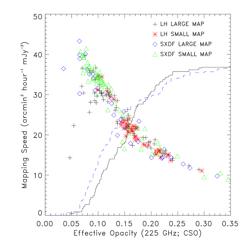
The AzTEC/SHADES observing strategy is similar to that used for other AzTEC blank-field surveys at the JCMT and is described in detail in previous publications (Scott et al., 2008; Perera et al., 2008). All observations were made while scanning the telescope in elevation in a raster pattern (see Wilson et al., 2008). Initially, the AzTEC/SHADES observations were made as small 15 arcmin $\times$ 15 arcmin mosaic maps with scan speeds of 90–120 arcsec s^-1. Later observations were extended to cover an entire field in one continuous observation of size 35 arcmin $\times$ 35 arcmin, which served to reduce observational overheads. Faster scan speeds of 180–220 arcsec s^-1 were used for these longer scans, which increased the effective sensitivity of the observations due to the corresponding reduction in residual atmospheric noise at the higher temporal frequencies (Wilson et al., 2008). After full reduction, the larger maps with faster scan-speeds have an observing efficiency of $\sim$ 150 per cent, relative to the smaller maps. In the end, 46 (63) mosaic maps and 65 (34) full maps were used to create the final LH (SXDF) map. These observations were performed over a wide range of atmospheric conditions and elevations. Figure 1 shows both the achieved mapping speeds and the cumulative distribution of observation time as a function of effective opacity at 225 GHz.

Nightly overhead observations included focusing, load curves, beam maps and pointing observations, all of which are described in the AzTEC instrument paper (Wilson et al., 2008). Pointing observations of bright point sources (typically $>1$ Jy) that lie near the science field being targeted were made every two hours. These measurements provide small corrections to the JCMT pointing model and are applied using a linear interpolation between the nearest pointing measurements taken before and after each science observation. Flux calibration is performed as described in Wilson et al. (2008) using the nightly load curves and beam maps of our primary calibration source, Uranus. The error in flux calibration is estimated to be 6–13 per cent on an individual observation (Wilson et al., 2008). The actual error in the final co-added AzTEC/SHADES maps, which comprise observations spanning many nights and calibrations, will be smaller, assuming the calibration uncertainty is randomly distributed. These individual error estimates do not include the systematic 5 per cent absolute uncertainty in the flux density of Uranus (Griffin & Orton, 1993).

Figure 1: Achieved mapping speeds for the various AzTEC/SHADES observations. Mapping speeds do not include overheads and are calculated as defined in Wilson et al. (2008). The cumulative distributions of observation time going into the final AzTEC/LH (92 hours) and AzTEC/SXDF (61 hours) maps are plotted as the solid and dashed curves, respectively, and normalised to an arbitrary value on the y-axis.

(a) Lockman Hole East (LH)

(b) Subaru/XMM-Newton Deep Field (SXDF)

Figure 2: AzTEC Signal-to-Noise maps of the Lockman Hole East field and SXDF, each observed with an AzTEC/JCMT beamsize of $\textrm{FWHM}\approx 18$ arcsec. Maps are displayed at different scales. The most significant source candidates, as defined in the text and listed in Tables 1–3, are circled. The observing pattern results in maps that are deepest in the centre, with noise increasing towards the edges. Reference contours show the distribution of 1$\sigma$ depth, in mJy. The maximal extent ($\sigma_{850}\leq 6$ mJy) of the overlapping 850–$\micron$ SCUBA/SHADES survey is depicted by the dotted curves. (a) AzTEC/LH $S/N$ map with 0.45 deg² total displayed area. For analysis purposes, the survey area is trimmed to the region of relatively uniform coverage (thick 1.3 mJy contour), resulting in a 0.31 deg² map with noise levels 0.9–1.3 mJy. For comparison in Section 5, the approximate size of the similar depth 1.1–mm AzTEC/GOODS-N survey (0.068 deg²; Perera et al., 2008) is represented by the dash-dotted rectangle; however, these surveys do not actually overlap on the sky. (b) AzTEC/SXDF $S/N$ map covering a total of 0.59 deg², with the trimmed analysis region (thick 1.7 mJy contour) covering 0.37 deg² with noise levels 1.0–1.7 mJy.

3 Maps and Catalogues

In this section we describe the methods used to construct the 1.1–mm maps and source catalogues. We test the astrometry and calibration of our maps against complementary radio data. We also describe expanded and improved methods for estimating and correcting for flux biases inherent to these surveys and test these estimates against simulations.

3.1 Mapmaking

The time streams of each observation are cleared of intermittent spikes (e.g. cosmic-ray events, instrumental glitches) and have the dominant atmospheric signals removed using the techniques described in Scott et al. (2008). Each observation is then mapped to a 3 arcsec $\times$ 3 arcsec grid in RA-Dec that is tangent to the celestial sphere at (10${}^{\textrm{h}}$51${}^{\textrm{m}}$59${}^{\textrm{s}}$, $+57^{\circ}$21^′43^′′) for Lockman Hole and (02${}^{\textrm{h}}$18${}^{\textrm{m}}$01${}^{\textrm{s}}$, $-04^{\circ}$59^′54^′′) for SXDF. These are the same pixel sizes and tangent points used for the SCUBA/SHADES 850–$\micron$ maps, allowing for straightforward comparison of maps in upcoming SHADES publications. All observations are then ‘co-added’ on the same grid to provide a weighted-average signal map and weight map for each field.

In parallel, we pass a simulated point source (as defined through beam map observations) through the same algorithms to trace and record the effective PSF, or ‘point source kernel’, in our final maps. We also create five noise-only map realisations of each observation by jack-knifing (randomly multiplying by $1$ or $-1$) each scan (5–15 seconds of data) of the time stream. This process works to remove any astronomical signal while preserving the dominant noise properties in the map. The resulting jack-knifed maps are dominated by residual atmospheric contamination and detector noise. One-hundred fully co-added noise maps are then created by randomly selecting a noise realisation for each observation and calculating the weighted average in the same manner used to create the co-added signal maps. Because the atmospheric contamination and the detector noise are uncorrelated amongst the full set of maps, the resulting co-added noise maps are, like the underlying noise in the signal map, extremely Gaussian.

Figure 3: Pixel $S/N$ histograms of the LH and SXDF maps (thick histograms) and average of their respective noise map realisations (thin histograms). The noise-only maps are well described as a Gaussian (smooth curve), while the signal maps are distorted by the presence of sources. Sources affect both the positive and negative flux distribution due to the zero-mean (AC-coupled) nature of these AzTEC maps. The distortions caused by sources are more apparent in LH due to the map’s lower average noise level compared to SXDF (Figure 2).

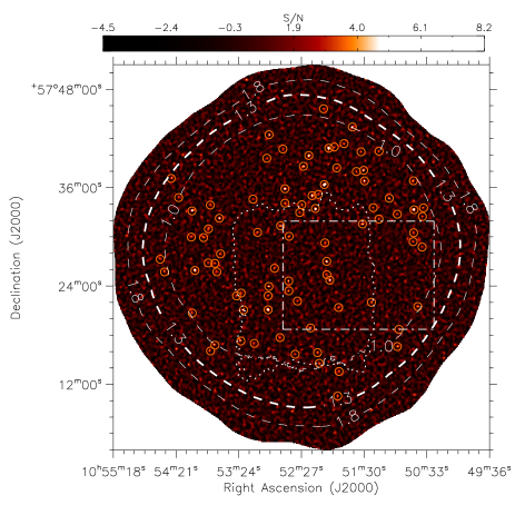
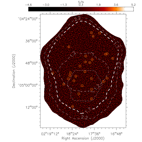
An optimal point source filter is applied to our maps utilising the information contained within the point source kernel and noise map realisations. The filtering techniques used are described in detail in previous AzTEC publications (Scott et al., 2008; Perera et al., 2008). The resulting AzTEC signal-to-noise maps of Lockman Hole and SXDF are shown in Fig. 2. The thick dashed contour of each map depicts the 50 per cent coverage level, representing a uniformly-covered region that has a noise level within $\sqrt{2}$ of that found in the deep central region of that map and beyond which the survey depth drops off sharply – a consequence of the particular observation modes employed. The AzTEC/SHADES maps are trimmed at this 50 per cent coverage level – as defined by the co-added weight map described above – for all analysis in the following sections. The trimmed maps have total sizes of 0.31 deg² and 0.37 deg² for LH and SXDF, respectively, and correspond to depths of $0.9<\sigma_{\textrm{lh}}<1.3$ mJy and $1.0<\sigma_{\textrm{sxdf}}<1.7$ mJy. The SXDF map is larger and shallower than that of Lockman Hole due to an observation script error that led to some individual maps being offset in declination. We continued to observe the resulting extended SXDF region after discovery of the error in order to maximise the usefulness of our entire data set.

The optimal filter is also applied to the co-added point source kernel and noise maps in order to provide the best model of the point source response and accurate estimates of the noise properties in our final maps. As shown for previously published AzTEC/JCMT maps (Scott et al., 2008; Perera et al., 2008), these noise-only maps confirm a highly Gaussian nature of the underlying noise in the AzTEC/SHADES data (see Figure 3). Accurate representations of the filtered point source kernel and the noise properties of the maps are critical components of the simulations described throughout this paper.

3.2 Astrometry

We have checked the astrometric accuracy of the AzTEC/SHADES maps by stacking (i.e. averaging) the AzTEC flux at the positions of radio sources in these fields (techniques described in detail in Scott et al., 2008). We use a re-reduction of the archival VLA 1.4 GHz continuum data in the Lockman Hole field (Ibar et al., 2009) to generate a catalogue of radio sources in the AzTEC/LH field and we utilise the 100 $\mu$Jy catalogue of Simpson et al. (2006) in the AzTEC/SXDF field. These catalogues result in stacked detections of significance 11 $\sigma$ and 7 $\sigma$ for AzTEC/LH and AzTEC/SXDF, respectively. The stacked data are consistent with no systematic astrometric offset in either map with the possible exception of a small offset in declination, $+2.9\pm 1.3$ arcsec, in the AzTEC/SXDF field. Due to the low significance and relatively small size of this potential offset, no correction is applied to the map.

We can also constrain the random astrometric errors across the AzTEC maps by measuring the broadening of the stacked signal compared to the AzTEC point-source response (see Scott et al., 2008). This broadening suggests that the random radial pointing error RMS is $\sigma_{\textrm{p}}\mathrel{\lower 2.5pt\vbox{\hbox{$<$}\hbox{$\sim$}}}4$ arcsec for both fields. Broadening of the stacked signal is also caused by pointing errors in individual AzTEC observations (final maps are co-additions of dozens of such observations) and clustering of the radio sources; therefore, $\sigma_{\textrm{p}}<4$ arcsec provides a strong upper limit to the random astrometric errors in the AzTEC/SHADES maps.

3.3 Calibration checks

Flux density calibration was performed on a nightly basis as described in Section 2. All steps in producing the AzTEC/SHADES maps were performed by the AzTEC instrument team (Wilson et al., 2008) and are identical to those employed for other published AzTEC data sets (Scott et al., 2008; Perera et al., 2008), thus minimising systematic differences between these AzTEC surveys. Flux calibration is expected to be consistent across all regions of the final AzTEC/SHADES maps, with each point being sampled numerous times by each of a large set ($\gg 10$) of observations that span a wide range of atmospheric conditions and calibrations.

We find no significant systematics between individual observations, including between the small mosaic and large full-map observations. Noise properties are consistent across individual observations, with mapping speeds following the correlation with atmospheric opacity described in Wilson et al. (2008). The methods used to remove atmospheric signal (Perera et al., 2008) produce consistent point source kernels (shape and amplitude) across all observations, with the resulting attenuation of point sources varying about the mean with an RMS of 3.6 per cent (attenuation corrected for in the final map based on the average reduction in flux density).

We also use the stacking analysis of Section 3.2 as a check of the relative calibrations between fields based on the average mm-wave flux of known radio populations. We find that the calibrations of the AzTEC/SHADES fields are consistent; the average 1.1–mm fluxes at the location of $S_{1.4\textrm{GHz}}>100$ $\mu$Jy radio sources are $0.59\pm 0.09$ mJy and $0.50\pm 0.07$ mJy for the LH and SXDF maps, respectively. If we remove radio sources that fall within 9 arcseconds of significant AzTEC ‘sources’ with $S/N\geq 3.5$ or $S/N\leq-3.5$ from the stacking analysis, we find that the stacked average 1.1–mm flux becomes $400\pm 100\,\mu$Jy and $430\pm 70\,\mu$Jy for LH and SXDF, respectively. We also utilise the deeper radio catalogue available for the LH field to determine that the average 1.1–mm flux of millimetre-dim $S_{1.4\textrm{GHz}}>66\,\mu$Jy radio sources is $528\pm 71\,\mu$Jy, which is consistent with similar stacks of the AzTEC/COSMOS ($530\pm 87\,\mu$Jy; Scott et al., 2008) and AzTEC/GOODS-N ($439\pm 107\,\mu$Jy; using the radio catalogue of Biggs & Ivison, 2006 and the AzTEC map of Perera et al., 2008) surveys. Assuming the various fields have similar radio populations, which may not be strictly true for fields with significant structure (e.g. AzTEC/COSMOS; Austermann et al., 2009), these tests show that the calibration across various AzTEC surveys is consistent within the measurement errors of the stacks. Note that since the available radio catalogue does not cover the entire AzTEC/LH field, we stack only on radio sources found in deep regions of the radio survey ($\sigma_{1.4\textrm{GHz}}<13\,\mu$Jy) to ensure a uniform sampling of $S_{1.4\textrm{GHz}}>66\,\mu$Jy sources.

3.4 Catalogues

Candidate mm-wave sources are identified as local maxima in the optimally filtered maps that pass a chosen threshold. Although it is possible that some local maxima could be due to multiple neighbouring sources (relative to the FWHM $\approx 18$ arcsec beamsize) that blend into one peak, the low $S/N$ of most detections prohibits deconvolution of potential multi-source peaks. AzTEC maps are mean-subtracted (i.e. the background has a zero net contribution) and SMGs are expected to be sparse, with less than one source per AzTEC/JCMT beam down to $<0.1$ mJy; therefore, source blending is expected to be rare for bright sources in the AzTEC/SHADES survey, unless the SMG population is significantly clustered on scales smaller than 18 arcseconds. Since very little is known about the SMG population on these scales, we caution the reader that the following analysis assumes no clustering at small scales. Interferometric observations over the coming years with the SMA, CARMA, and later with ALMA will address the clustering question definitively.

The most robust AzTEC/SHADES source candidates are given in Tables 1–3. Source candidates are listed in descending order of detected $S/N$. Centroid source positions are determined using flux-squared weighting of the pixels within 9 arcsec (FWHM/2) of the local maxima. The AzTEC/SHADES survey detects 43 and 21 robust sources with $S/N\geq 4$ in the LH and SXDF fields, respectively. Additional significant detections, as defined in Section 3.6, are also listed in the source tables and considered in the analysis of Section 4. Multi-wavelength analysis of sources found in the AzTEC/SHADES survey, including combined 850 $\micron$/1100 $\micron$ properties of sources within the overlapping AzTEC and SCUBA SHADES surveys (Negrello et al., in prep.), is deferred to future publications.

3.5 Flux corrections

Figure 4: Bayesian posterior flux density (PFD; solid curve) compared to the intrinsic flux distribution recovered through simulation (histogram with 1$\sigma$ Poisson errors of simulation) for sources detected at the significance listed and at a noise level of $\sigma_{\textrm{m}}=1.0$ mJy. Also shown are the Bayesian predictions without the correction for the bias to peak locations in the map (dotted curves). The dashed vertical line represents the raw measured flux, $S_{\textrm{m}}$, while the dashed curve represents the Gaussian probability distribution that might otherwise be assumed without flux boosting and/or false detection considerations. Negative flux probabilities are allowable through the zero-mean AzTEC point-source kernel and effectively represent the probability of a null detection.

Sources discovered in these blind surveys experience two notable flux biases, both of which cause the average measurement of the flux density of a detected source to be high relative to its true intrinsic flux, $S_{\textrm{i}}$. These flux biases can be very significant ($\sim$ 10–50 per cent for sources listed in Tables 1–3), particularly for the low-significance detections that typify SMG surveys. Therefore, it is important to characterise and correct for these biases before fluxes and number counts can be compared to measurements at other wavelengths. Since these biases are a function of survey depth, these corrections are also necessary before detailed comparisons can be made with other 1.1 mm surveys.

Table 1: AzTEC Lockman Hole (LH) candidates with $S/N\geq 4$. Additional robust AzTEC/LH sources with lower $S/N$ values are listed in Table 2. The columns give: 1) AzTEC source name, including RA/DEC centroid position; 2) Nickname; 3) Signal-to-noise of the detection in the AzTEC map; 4) Measured 1100–$\micron$ flux density and error; 5) Flux density and 68 per cent confidence interval, as defined in Section 3.6, after corrections for flux boosting and the bias to peak locations in the map; 6) Probability that the source will de-boost to $S_{\textrm{i}}<0$ when assuming the AzTEC/SHADES Bayesian prior.

			$S_{1100}$	$S_{1100}$
			(measured)	(corrected)
Source	Nickname	$S/N$	(mJy)	(mJy)	$P(S_{1100}<0)$
AzTEC_J105201.98+574049.3	AzLOCK.1	8.2	$7.4\pm 0.9$	$6.6^{+0.9}_{-1.0}$	0.000
AzTEC_J105206.08+573622.6	AzLOCK.2	8.2	$7.2\pm 0.9$	$6.4^{+0.9}_{-0.9}$	0.000
AzTEC_J105257.18+572105.9	AzLOCK.3	7.5	$7.2\pm 1.0$	$6.2^{+1.1}_{-0.9}$	0.000
AzTEC_J105044.47+573318.3	AzLOCK.4	6.7	$6.2\pm 0.9$	$5.3^{+0.9}_{-1.0}$	0.000
AzTEC_J105403.76+572553.7	AzLOCK.5	6.4	$5.9\pm 0.9$	$4.9^{+1.0}_{-0.9}$	0.000
AzTEC_J105241.89+573551.7	AzLOCK.6	6.2	$5.6\pm 0.9$	$4.8^{+0.8}_{-1.0}$	0.000
AzTEC_J105203.89+572700.5	AzLOCK.7	6.0	$5.7\pm 0.9$	$4.8^{+0.9}_{-1.1}$	0.000
AzTEC_J105201.14+572443.0	AzLOCK.8	6.0	$5.6\pm 0.9$	$4.7^{+1.0}_{-1.0}$	0.000
AzTEC_J105214.22+573327.4	AzLOCK.9	5.7	$5.0\pm 0.9$	$4.1^{+0.9}_{-0.9}$	0.000
AzTEC_J105406.44+573309.6	AzLOCK.10	5.5	$5.1\pm 0.9$	$4.1^{+0.9}_{-1.0}$	0.000
AzTEC_J105130.29+573807.2	AzLOCK.11	5.4	$4.8\pm 0.9$	$3.8^{+1.0}_{-0.9}$	0.000
AzTEC_J105217.23+573501.4	AzLOCK.12	5.4	$4.7\pm 0.9$	$3.8^{+0.9}_{-1.0}$	0.000
AzTEC_J105140.64+574324.6	AzLOCK.13	5.3	$5.3\pm 1.0$	$4.1^{+1.0}_{-1.1}$	0.000
AzTEC_J105220.24+573955.1	AzLOCK.14	5.2	$4.6\pm 0.9$	$3.6^{+0.9}_{-0.9}$	0.000
AzTEC_J105256.32+574227.5	AzLOCK.15	5.2	$4.8\pm 0.9$	$3.7^{+0.9}_{-1.0}$	0.000
AzTEC_J105341.50+573215.9	AzLOCK.16	5.2	$4.7\pm 0.9$	$3.7^{+1.0}_{-1.0}$	0.000
AzTEC_J105319.47+572105.3	AzLOCK.17	5.0	$4.7\pm 0.9$	$3.6^{+1.0}_{-1.0}$	0.001
AzTEC_J105225.16+573836.7	AzLOCK.18	4.8	$4.2\pm 0.9$	$3.2^{+1.0}_{-0.9}$	0.001
AzTEC_J105129.55+573649.2	AzLOCK.19	4.8	$4.3\pm 0.9$	$3.2^{+1.0}_{-0.9}$	0.002
AzTEC_J105345.53+571647.0	AzLOCK.20	4.7	$4.7\pm 1.0$	$3.4^{+1.1}_{-1.1}$	0.004
AzTEC_J105131.41+573134.1	AzLOCK.21	4.7	$4.1\pm 0.9$	$3.1^{+0.9}_{-1.0}$	0.003
AzTEC_J105256.49+572356.7	AzLOCK.22	4.7	$4.5\pm 1.0$	$3.2^{+1.1}_{-1.0}$	0.004
AzTEC_J105321.96+571717.8	AzLOCK.23	4.5	$4.4\pm 1.0$	$3.1^{+1.0}_{-1.1}$	0.007
AzTEC_J105238.46+572436.8	AzLOCK.24	4.5	$4.3\pm 0.9$	$3.0^{+1.0}_{-1.1}$	0.007
AzTEC_J105107.06+573442.2	AzLOCK.25	4.4	$3.9\pm 0.9$	$2.7^{+1.0}_{-0.9}$	0.008
AzTEC_J105059.75+571636.7	AzLOCK.26	4.3	$4.6\pm 1.0$	$3.1^{+1.1}_{-1.3}$	0.016
AzTEC_J105218.64+571852.9	AzLOCK.27	4.3	$4.3\pm 1.0$	$2.9^{+1.1}_{-1.1}$	0.013
AzTEC_J105045.11+573650.4	AzLOCK.28	4.3	$4.1\pm 1.0$	$2.7^{+1.1}_{-1.1}$	0.015
AzTEC_J105123.33+572200.8	AzLOCK.29	4.2	$4.0\pm 0.9$	$2.7^{+1.1}_{-1.1}$	0.016
AzTEC_J105238.09+573003.4	AzLOCK.30	4.2	$3.8\pm 0.9$	$2.6^{+0.9}_{-1.1}$	0.014
AzTEC_J105425.31+573707.8	AzLOCK.31	4.2	$5.2\pm 1.2$	$3.1^{+1.4}_{-1.6}$	0.038
AzTEC_J105041.16+572129.6	AzLOCK.32	4.2	$4.1\pm 1.0$	$2.7^{+1.1}_{-1.2}$	0.020
AzTEC_J105245.93+573121.2	AzLOCK.33	4.2	$3.8\pm 0.9$	$2.5^{+1.0}_{-1.0}$	0.016
AzTEC_J105238.35+572324.4	AzLOCK.34	4.1	$4.0\pm 1.0$	$2.6^{+1.0}_{-1.2}$	0.023
AzTEC_J105355.84+572954.7	AzLOCK.35	4.1	$3.7\pm 0.9$	$2.5^{+1.0}_{-1.1}$	0.021
AzTEC_J105349.58+571604.3	AzLOCK.36	4.1	$4.3\pm 1.1$	$2.7^{+1.2}_{-1.3}$	0.032
AzTEC_J105152.72+571334.5	AzLOCK.37	4.1	$4.1\pm 1.0$	$2.6^{+1.1}_{-1.3}$	0.033
AzTEC_J105116.44+573209.9	AzLOCK.38	4.0	$3.5\pm 0.9$	$2.4^{+1.0}_{-1.1}$	0.025
AzTEC_J105212.26+571552.5	AzLOCK.39	4.0	$4.0\pm 1.0$	$2.5^{+1.1}_{-1.3}$	0.035
AzTEC_J105226.58+573355.0	AzLOCK.40	4.0	$3.5\pm 0.9$	$2.3^{+1.0}_{-1.0}$	0.026
AzTEC_J105116.34+574027.3	AzLOCK.41	4.0	$3.7\pm 0.9$	$2.4^{+1.1}_{-1.2}$	0.036
AzTEC_J105058.27+571842.8	AzLOCK.42	4.0	$3.9\pm 1.0$	$2.4^{+1.2}_{-1.2}$	0.042
AzTEC_J105153.10+572122.7	AzLOCK.43	4.0	$3.8\pm 1.0$	$2.4^{+1.1}_{-1.2}$	0.039

Table 2: AzTEC/LH source candidates with $S/N<4$. Columns as described in Table 1.

			$S_{1100}$	$S_{1100}$
			(measured)	(corrected)
Source	Nickname	$S/N$	(mJy)	(mJy)	$P(S_{1100}<0)$
AzTEC_J105241.87+573406.1	AzLOCK.44	3.9	$3.5\pm 0.9$	$2.3^{+1.0}_{-1.1}$	0.033
AzTEC_J105154.82+573824.6	AzLOCK.45	3.9	$3.5\pm 0.9$	$2.2^{+1.0}_{-1.1}$	0.035
AzTEC_J105210.75+571433.8	AzLOCK.46	3.9	$3.9\pm 1.0$	$2.4^{+1.2}_{-1.3}$	0.047
AzTEC_J105306.80+573032.7	AzLOCK.47	3.9	$3.6\pm 0.9$	$2.3^{+1.0}_{-1.2}$	0.037
AzTEC_J105431.31+572543.3	AzLOCK.48	3.9	$4.0\pm 1.0$	$2.4^{+1.3}_{-1.3}$	0.052
AzTEC_J105340.49+572755.0	AzLOCK.49	3.9	$3.6\pm 0.9$	$2.2^{+1.1}_{-1.1}$	0.039
AzTEC_J105205.59+572916.1	AzLOCK.50	3.9	$3.5\pm 0.9$	$2.2^{+1.0}_{-1.2}$	0.042
AzTEC_J105035.90+573332.1	AzLOCK.51	3.9	$3.7\pm 1.0$	$2.2^{+1.2}_{-1.2}$	0.050
AzTEC_J105206.79+574537.5	AzLOCK.52	3.9	$4.2\pm 1.1$	$2.4^{+1.3}_{-1.6}$	0.070
AzTEC_J105435.20+572715.9	AzLOCK.53	3.9	$4.0\pm 1.0$	$2.4^{+1.2}_{-1.5}$	0.062
AzTEC_J105351.57+572648.8	AzLOCK.54	3.8	$3.5\pm 0.9$	$2.1^{+1.1}_{-1.2}$	0.050
AzTEC_J105153.94+571034.3	AzLOCK.55	3.8	$4.6\pm 1.2$	$2.4^{+1.3}_{-2.0}$	0.094
AzTEC_J105203.84+572522.7	AzLOCK.56	3.8	$3.6\pm 0.9$	$2.1^{+1.1}_{-1.3}$	0.055
AzTEC_J105251.38+572609.9	AzLOCK.57	3.8	$3.6\pm 0.9$	$2.1^{+1.2}_{-1.2}$	0.056
AzTEC_J105243.78+574042.6	AzLOCK.58	3.8	$3.4\pm 0.9$	$2.1^{+1.1}_{-1.2}$	0.053
AzTEC_J105044.92+573030.0	AzLOCK.59	3.8	$3.4\pm 0.9$	$2.1^{+1.1}_{-1.2}$	0.054
AzTEC_J105345.63+572645.8	AzLOCK.60	3.8	$3.5\pm 0.9$	$2.1^{+1.1}_{-1.2}$	0.056
AzTEC_J105257.19+572248.5	AzLOCK.61	3.8	$3.7\pm 1.0$	$2.1^{+1.2}_{-1.3}$	0.063
AzTEC_J105211.61+573510.7	AzLOCK.62	3.8	$3.3\pm 0.9$	$2.0^{+1.0}_{-1.2}$	0.056
AzTEC_J105406.14+572042.0	AzLOCK.63	3.7	$3.7\pm 1.0$	$2.1^{+1.2}_{-1.4}$	0.074
AzTEC_J105310.94+573435.6	AzLOCK.64	3.7	$3.3\pm 0.9$	$2.0^{+1.1}_{-1.2}$	0.059
AzTEC_J105258.39+573935.4	AzLOCK.65	3.7	$3.4\pm 0.9$	$2.0^{+1.1}_{-1.2}$	0.061
AzTEC_J105351.46+573058.2	AzLOCK.66	3.7	$3.4\pm 0.9$	$2.0^{+1.1}_{-1.2}$	0.064
AzTEC_J105045.33+572924.4	AzLOCK.67	3.7	$3.4\pm 0.9$	$1.9^{+1.1}_{-1.2}$	0.065
AzTEC_J105325.86+572247.3	AzLOCK.68	3.7	$3.5\pm 0.9$	$2.0^{+1.1}_{-1.3}$	0.071
AzTEC_J105059.74+573245.6	AzLOCK.69	3.7	$3.3\pm 0.9$	$1.9^{+1.1}_{-1.2}$	0.064
AzTEC_J105121.65+573333.6	AzLOCK.70	3.7	$3.2\pm 0.9$	$1.9^{+1.0}_{-1.2}$	0.064
AzTEC_J105407.02+572957.7	AzLOCK.71	3.7	$3.4\pm 0.9$	$1.9^{+1.1}_{-1.3}$	0.071
AzTEC_J105132.73+574022.1	AzLOCK.72	3.7	$3.4\pm 0.9$	$1.9^{+1.1}_{-1.2}$	0.069
AzTEC_J105157.08+574057.6	AzLOCK.73	3.7	$3.3\pm 0.9$	$1.9^{+1.1}_{-1.2}$	0.068
AzTEC_J105246.38+571742.5	AzLOCK.74	3.7	$3.6\pm 1.0$	$1.9^{+1.2}_{-1.4}$	0.087
AzTEC_J105309.72+571700.1	AzLOCK.75	3.7	$3.6\pm 1.0$	$1.9^{+1.2}_{-1.4}$	0.087
AzTEC_J105228.45+573258.0	AzLOCK.76	3.7	$3.2\pm 0.9$	$1.9^{+1.0}_{-1.2}$	0.067
AzTEC_J105148.13+574122.5	AzLOCK.77	3.7	$3.3\pm 0.9$	$1.9^{+1.1}_{-1.3}$	0.073
AzTEC_J105349.75+573352.4	AzLOCK.78	3.7	$3.4\pm 0.9$	$1.9^{+1.1}_{-1.3}$	0.076
AzTEC_J105232.60+571540.3	AzLOCK.79	3.7	$3.6\pm 1.0$	$1.9^{+1.2}_{-1.5}$	0.088
AzTEC_J105418.55+573447.5	AzLOCK.80	3.7	$3.7\pm 1.0$	$1.9^{+1.1}_{-1.5}$	0.093
AzTEC_J105321.70+572308.3	AzLOCK.81	3.6	$3.4\pm 0.9$	$1.9^{+1.1}_{-1.4}$	0.083
AzTEC_J105136.91+573758.1	AzLOCK.82	3.6	$3.2\pm 0.9$	$1.8^{+1.0}_{-1.3}$	0.079
AzTEC_J105343.81+572543.6	AzLOCK.83	3.6	$3.3\pm 0.9$	$1.8^{+1.0}_{-1.4}$	0.090
AzTEC_J105230.53+572210.0	AzLOCK.84	3.6	$3.4\pm 1.0$	$1.8^{+1.0}_{-1.6}$	0.099
AzTEC_J105036.93+573228.9	AzLOCK.85	3.6	$3.3\pm 0.9$	$1.8^{+1.0}_{-1.5}$	0.096
AzTEC_J105037.18+572844.9	AzLOCK.86	3.6	$3.3\pm 0.9$	$1.7^{+0.9}_{-1.5}$	0.099

Table 3: AzTEC/SXDF source candidates. Columns as described in Table 1.

			$S_{1100}$	$S_{1100}$
			(measured)	(corrected)
Source	Nickname	$S/N$	(mJy)	(mJy)	$P(S_{1100}<0)$
AzTEC_J021738.52$-$043330.3	AzSXDF.1	5.2	$7.4\pm 1.4$	$5.3^{+1.4}_{-1.7}$	0.002
AzTEC_J021745.76$-$044747.8	AzSXDF.2	4.8	$5.4\pm 1.1$	$4.0^{+1.1}_{-1.3}$	0.003
AzTEC_J021754.97$-$044723.9	AzSXDF.3	4.8	$5.3\pm 1.1$	$3.8^{+1.2}_{-1.2}$	0.004
AzTEC_J021831.27$-$043911.9	AzSXDF.4	4.8	$6.9\pm 1.4$	$4.4^{+1.7}_{-1.6}$	0.011
AzTEC_J021742.10$-$045626.7	AzSXDF.5	4.7	$5.1\pm 1.1$	$3.6^{+1.2}_{-1.2}$	0.005
AzTEC_J021842.39$-$045932.7	AzSXDF.6	4.6	$5.8\pm 1.3$	$4.0^{+1.3}_{-1.6}$	0.010
AzTEC_J021655.80$-$044532.2	AzSXDF.7	4.6	$6.3\pm 1.4$	$4.0^{+1.6}_{-1.7}$	0.019
AzTEC_J021742.13$-$043135.6	AzSXDF.8	4.5	$6.4\pm 1.4$	$4.0^{+1.6}_{-1.8}$	0.025
AzTEC_J021823.10$-$051136.7	AzSXDF.9	4.3	$6.9\pm 1.6$	$3.8^{+1.9}_{-2.4}$	0.061
AzTEC_J021816.07$-$045512.2	AzSXDF.10	4.3	$4.7\pm 1.1$	$3.1^{+1.2}_{-1.3}$	0.018
AzTEC_J021708.04$-$045615.3	AzSXDF.11	4.3	$5.5\pm 1.3$	$3.3^{+1.5}_{-1.7}$	0.039
AzTEC_J021708.03$-$044256.8	AzSXDF.12	4.2	$5.9\pm 1.4$	$3.3^{+1.7}_{-1.9}$	0.053
AzTEC_J021829.13$-$045448.2	AzSXDF.13	4.2	$4.4\pm 1.1$	$2.8^{+1.2}_{-1.4}$	0.028
AzTEC_J021740.55$-$044609.1	AzSXDF.14	4.1	$4.8\pm 1.2$	$2.9^{+1.3}_{-1.5}$	0.037
AzTEC_J021754.76$-$044417.5	AzSXDF.15	4.1	$4.8\pm 1.2$	$2.9^{+1.3}_{-1.5}$	0.037
AzTEC_J021716.24$-$045808.4	AzSXDF.16	4.1	$5.0\pm 1.2$	$2.9^{+1.5}_{-1.6}$	0.044
AzTEC_J021711.62$-$044315.1	AzSXDF.17	4.1	$5.6\pm 1.4$	$3.1^{+1.6}_{-2.0}$	0.064
AzTEC_J021724.48$-$043144.5	AzSXDF.18	4.1	$6.1\pm 1.5$	$3.1^{+1.5}_{-2.6}$	0.091
AzTEC_J021906.24$-$045333.4	AzSXDF.19	4.0	$6.5\pm 1.6$	$3.3^{+0.9}_{-3.3}$	0.118a
AzTEC_J021742.13$-$050723.4	AzSXDF.20	4.0	$5.7\pm 1.4$	$2.9^{+1.3}_{-2.6}$	0.096
AzTEC_J021809.81$-$050444.8	AzSXDF.21	4.0	$5.0\pm 1.3$	$2.6^{+1.6}_{-1.8}$	0.070
AzTEC_J021827.89$-$045320.5	AzSXDF.22	3.9	$4.2\pm 1.1$	$2.5^{+1.2}_{-1.5}$	0.057
AzTEC_J021820.23$-$045738.7	AzSXDF.23	3.9	$4.3\pm 1.1$	$2.5^{+1.3}_{-1.6}$	0.060
AzTEC_J021832.33$-$045632.7	AzSXDF.24	3.8	$4.1\pm 1.1$	$2.3^{+1.3}_{-1.5}$	0.065
AzTEC_J021802.42$-$050018.4	AzSXDF.25	3.8	$4.2\pm 1.1$	$2.3^{+1.2}_{-1.7}$	0.081
AzTEC_J021756.39$-$045242.5	AzSXDF.26	3.8	$4.0\pm 1.1$	$2.1^{+1.3}_{-1.5}$	0.076
AzTEC_J021741.50$-$050218.0	AzSXDF.27	3.8	$4.4\pm 1.2$	$2.3^{+1.1}_{-2.0}$	0.096
AzTEC_J021806.97$-$044941.9	AzSXDF.28	3.7	$3.9\pm 1.1$	$2.0^{+1.1}_{-1.7}$	0.091

Notes: $a)$ Source is included in order to have a complete list of candidates with $S/N$ $\geq$ 4, despite its relatively high null probability.

The primary flux bias in SMG surveys is commonly referred to as ‘flux boosting’ and is due to the combination of a source density that increases sharply with decreasing flux and the blind nature of the survey (i.e. sources have previously unknown positions); see Hogg & Turner (1998) for a full description of this effect. We employ an advanced version of the Bayesian methods of Coppin et al. (2005, 2006) to correct for flux boosting and generate a full posterior flux density (PFD) probability distribution for each source candidate. The Bayesian approach requires a prior in the form of the assumed number density of sources projected on the sky (i.e. ‘number counts’) as a function of flux. We use the iterative method of Austermann et al. (2009) to determine the most appropriate prior. We begin by using the SCUBA/SHADES (Coppin et al., 2006) 850–$\micron$ number counts, scaled to 1.1 mm through an initial assumption of the 850/1100 $\micron$ flux ratio, as the initial prior. The prior is then iteratively adjusted using the empirical number counts of this survey (Section 4.1), which quickly converges within a few iterations. As the widest-area deep millimetre survey to date, these iterative AzTEC/SHADES results provide the best 1.1–mm blank-field source number density prior available.

A second notable flux bias results from sources being defined as local maxima in the map. Since the position of the source is not independently known, nearby positive noise inevitably induces positional errors and this noise can combine with the off-centre beam-convolved flux of the source to outshine the true source being measured, thus resulting in an average positive flux bias in the local maximum that is taken as the measurement. The bias is independent of the aforementioned ‘flux boosting’ (the Bayesian prior is a noiseless calculation) and is instead a systematic of the actual measurement, as opposed to an effect of the luminosity function being surveyed. This bias to peaks (or ‘noise gradient bias’, e.g. Ivison et al., 2007) is minimised by optimally filtering the map for point sources, but can still be a significant factor for low-significance sources.

We characterise and quantify the bias to peak locations through 10,000 simulations of the LH and SXDF maps. These simulated maps are generated by populating the noise-only maps with the flux-scaled point source kernel at random locations drawn from a uniform distribution and in accordance with a number counts distribution that is consistent with the final AzTEC/SHADES counts (Section 4.1). We generate simulated PFDs by cataloguing the input flux ($S_{\textrm{i}}$) associated with each source measurement ($S_{\textrm{m}}$,$\sigma_{\textrm{m}}$) recovered in the simulated maps. These simulated PFDs are compared to the Bayesian estimate to characterise the remaining bias (e.g. Fig. 4), which comes primarily from the bias to peak locations. Through comparison of the PFDs over the flux range under investigation here ($S_{\textrm{i}}>$ 1 mJy) and for detections with $S/N\geq$ 3 , we find that the average flux bias incurred for an AzTEC/JCMT measurement of ($S_{\textrm{m}}$,$\sigma_{\textrm{m}}$) is well described by the equation

$${b_{\mathrm{peak}}(S_{\textrm{m}},\sigma_{\textrm{m}})}={{\alpha\sigma_{\textrm{m}}}\over\sqrt{2\pi}}\exp{\left({-{\beta^{2}S_{\textrm{m}}^{2}}}\over{2\sigma_{\textrm{m}}^{2}}\right)}$$ (1)

with $\alpha=1$ and $\beta=0.4$. In this form, the bias is modelled as $\alpha$ effective independent noise elements that lie at a radial distance from the true source that is equivalent to that where the fractional flux of the Gaussian beam (relative to maximum) is $\beta$. Although this bias is relatively small in flux, it can have a strong effect on the Bayesian probability densities of low $S/N$ detections (e.g. 50 per cent overestimate in probability that $S_{\textrm{i}}=S_{\textrm{m}}$ for a $S_{\textrm{m}}=3\pm 1$ mJy measurement; see Fig. 4). We note that the estimates provided by Equation 1 are significantly smaller than the generalised case provided by Equation B19 of Ivison et al. (2007) and are specifically tailored to AzTEC/JCMT scanning observations through simulation. Maps with a significantly different response to point sources (e.g. different beamsize or mapping strategy) may require a reevaluation of the functional form and parameter values of Equation 1.

We correct for the bias to peak locations by subtracting $b_{\textrm{peak}}$ from the measured flux, $S_{\textrm{m}}$, before calculating the Bayesian estimated PFD. The differences between the Bayesian PFDs with (solid curves) and without (dashed curves) this secondary bias correction can be seen in Fig. 4 for several $S/N$ detection levels. Analysis of past surveys typically ignored this bias, but largely avoided its effects by restricting the analysis to only the most significant sources (e.g. $S/N$ $\mathrel{\lower 2.5pt\vbox{\hbox{$>$}\hbox{$\sim$}}}$ 4).

The de-boosted flux value listed for each source in Tables 1–3 is taken as the flux at the PFD local maximum nearest the detected flux, $S_{\textrm{m}}$ (see Fig. 4). Our improved estimate of the significant biases at work for low significance detections leads to accurate PFDs down to at least $S/N=3$, thus allowing us to utilise more of the maps’ information when conducting the source-list driven number counts analysis of Section 4.

3.6 Source robustness and false detections

The effects of flux boosting (Section 3.5) make $S/N$ a less than ideal measure of source robustness; therefore, we include an estimate of the total probability that the source will de-boost to $S_{\textrm{i}}<0$, $P(S_{1100}<0)$, as determined from the integrated Bayesian PFD, in the source lists of Tables 1–3. This provides a better metric than just $S/N$ for the relative robustness of the source detections, due to its dependence on both $S_{\textrm{m}}$ and $\sigma_{\textrm{m}}$, rather than just the ratio $S_{\textrm{m}}/\sigma_{\textrm{m}}$ (see also Coppin et al., 2006). We have restricted Tables 1–3 to include only the most robust AzTEC/SHADES sources with $P(S_{1100}<0)\leq 0.1$. The effective $S/N$, as a function of $\sigma_{\textrm{m}}$, of this 10 per cent ‘null-threshold’ is plotted in Fig. 5. We note that the absolute value of $P(S_{1100}<0)$ is highly sensitive to the Bayesian prior used. For example, if we instead assumed the results of the relatively source-rich AzTEC/GOODS-N survey (Perera et al., 2008) as the Bayesian prior, the number of sources in AzTEC/LH passing the 10 per cent null-threshold increases from 86 to 221. Therefore, it is important to consider the priors used when comparing the number of ‘detections’ in various surveys of this type. However, we note that the effect of the choice of prior on the resulting number counts (Section 4) is much less substantial, as the apparent change in the number of ‘detections’ is largely counteracted by the survey completeness corresponding to the particular prior used.

Figure 5: Effective $S/N$ threshold as a function of noise level for the given null-threshold values when assuming the AzTEC/SHADES number counts as the Bayesian prior. These curves represent constant levels of robustness for an SMG detection using AzTEC/JCMT data. These values are unique to the particular Bayesian prior (number counts) assumed.

Figure 6: Ratio of the total number of detections to the number of significant noise-only peaks as a function of null-threshold for the 50 per cent coverage region of AzTEC/LH and AzTEC/SXDF. This provides an estimate of the relative number of false detections expected beyond a given source threshold, i.e. below a given null-threshold.

The number of false detections in a given source catalogue depends strongly on the chosen threshold for what is, and what is not, defined as a source. Due to the relatively large 18 arcsecond beamsize of AzTEC on the JCMT, the AzTEC/SHADES maps are expected to become significantly ‘full’ of sources (on average one source per beam) when considering the expected high density of sources with 1.1–mm fluxes $<0.1$ mJy. Various estimates of the false detection rate of AzTEC/JCMT maps are explored in Perera et al. (2008), who conclude that the average number of significant noise peaks in the jack-knifed noise-only maps provide a conservative overestimate of the number of false detections in the map (a consequence of true source signal adding both positive and negative fluxes to the underlying noise distribution to our zero-mean maps). The ratio of number of sources in the signal map to the average number found in the corresponding noise-only maps is plotted as a function of null-threshold in Fig. 6 for the LH and SXDF fields.

4 SMG Number Counts

In this section, we present the sky-projected densities of 1.1–mm sources in the AzTEC/SHADES survey and the methods by which they are determined. These methods represent an extended and improved version of the algorithms outlined in the SCUBA/SHADES number counts paper (Coppin et al., 2006). In Section 4.3 we provide parametric fits to the number count results of the combined surveys. These number count results provide a useful measure of the SMG population through which we compare those found in other fields, at different wavelengths, and that predicted by various models and simulations (Section 5).

4.1 Number counts: algorithm and results

We calculate source number counts using the bootstrap sampling methods outlined in Austermann et al. (2009), which are motivated by those used to determine the SCUBA/SHADES number counts (Coppin et al., 2006). In this method, the catalogues of continuous source PFDs are sampled at random and with replacement (e.g. Press et al., 1992) in order to determine specific intrinsic fluxes for the sources in the catalogue. These samples are binned to produce both differential and integral source counts as a function of intrinsic flux. This sampling process is repeated 100,000 times to provide sufficient sampling of the source count probability distribution. Sampling variance is injected by Poisson deviating the number of sources sampled in each of the 100,000 iterations around the actual number of sources detected in the map. Number count results are taken as the mean of each bin and the distribution across the iterations is used to characterise the associated uncertainty. The counts are then corrected for completeness, using estimates derived from simulation, and scaled for survey area. The resulting number counts are then taken as the new Bayesian prior and the entire process, including producing new catalogues of sources and their PFDs, is repeated in the iterative-prior process described in Section 3.5. For each iteration of the prior, the number counts are calculated for both the LH and SXDF surveys independently and also for the two surveys combined. The Bayesian prior chosen for the next iteration is always taken as the best fit to the combined result. This iterative procedure minimises our bias to the number counts assumed in the Bayesian calculations.

Previous surveys using a similar bootstrapping technique (Coppin et al., 2006; Perera et al., 2008; Austermann et al., 2009) limited the source catalogue to those sources with negative flux probability of $P(S_{\textrm{i}}<0)<0.05$, i.e. a null-threshold of 5 per cent. This null-threshold value was historically used to limit the number of false detections to a near negligible amount and to render the bias to peak locations relatively insignificant. However, the false detection probability is inherently accounted for in the bootstrap sampling method if accurate PFDs are used. As discussed in Section 3, our bias corrections result in PFDs that are accurate for all source candidates with $S/N\geq 3$, and possibly lower significance (currently untested below $S/N=3$). The PFDs are particularly accurate in the $S_{\textrm{i}}\geq 1$ mJy flux range considered in this analysis. Since the traditional null-threshold of 5 per cent would limit the AzTEC/SHADES source candidate list to just those with $S/N\mathrel{\lower 2.5pt\vbox{\hbox{$>$}\hbox{$\sim$}}}4$ (Fig. 5), we explore fainter sources in the data set with the use of higher null-thresholds that incorporate a larger catalogue of source candidates in the derivation of source count densities.

We derive combined AzTEC/SHADES number counts using null-thresholds of 5, 10, and 20 per cent. The 20 per cent threshold represents the lowest significance tested in our simulations (effective $S/N\mathrel{\lower 2.5pt\vbox{\hbox{$>$}\hbox{$\sim$}}}3$) and safely avoids complications related to source confusion by keeping the density of detections sufficiently low. The results are consistent for all three threshold values tested and the variations between the results are, in general, much smaller than the formal 68 per cent uncertainty of the number count estimates. We have verified through simulation that the use of the higher null-threshold values supplies additional data without introducing any significant biases or systematics (Section 4.2).

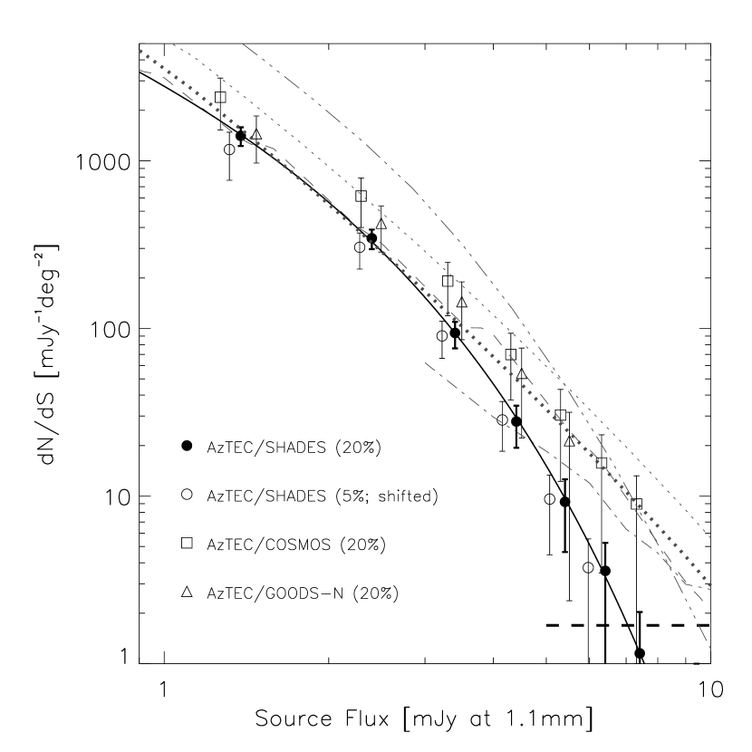
The combined AzTEC/SHADES differential number counts using 5 per cent (open circles) and 20 per cent (filled circles) thresholds are compared in Fig. 7. The two results are nearly identical at high fluxes, but differ slightly in the lower flux bins. The variation at low flux is not surprising given that the 180 additional source candidates being considered when using the softer 20 per cent threshold are all relatively low in flux, thus providing significantly more data in the lower flux bins. All AzTEC/SHADES number count uncertainties represent the 68 per cent confidence interval derived from the distribution of bootstrap iterations. All uncertainties assume a spatially random distribution of sources and, therefore, do not account for the effects of cosmic variance/clustering. The differential number counts data points are strongly correlated, as described in Appendix A.

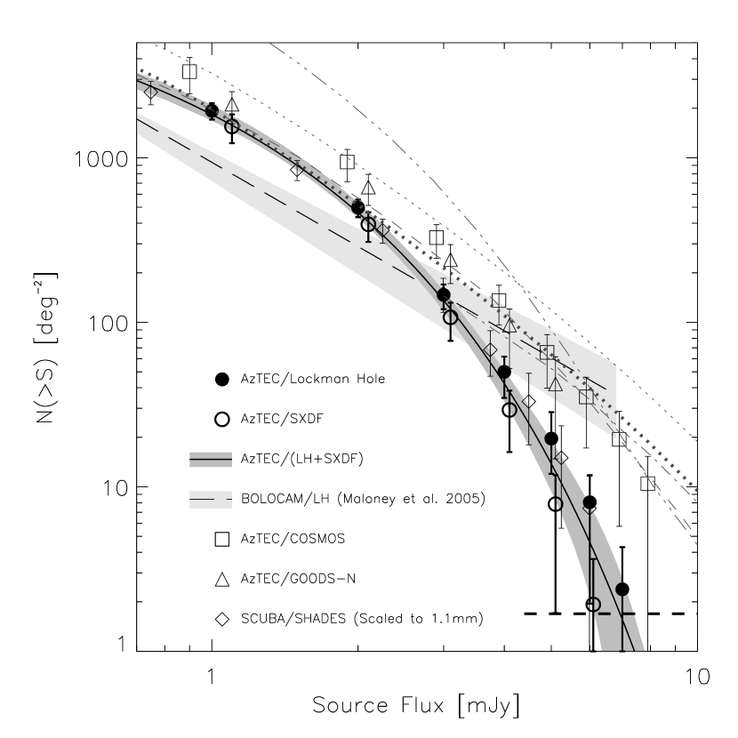
Fig. 8 presents the integral source counts, $N({>}\,S)$, for both the LH and SXDF surveys using the 20 per cent null-threshold. Unlike the finite-bin differential counts measurements, the integral counts are threshold measurements (i.e. number of sources greater than flux, $S$) and can be derived at continuous values of flux. Therefore, the final combined AzTEC/SHADES results are depicted as a continuous 68 per cent confidence region. The combined differential and integral number counts are also given in Table 4, with integral counts listed at integer flux limits.

Figure 7: Differential number counts for the combined AzTEC/SHADES survey in 1 mJy wide bins. The per cent value in parentheses represents the null-threshold used for each data set. The 5 per cent threshold results of AzTEC/SHADES have been artificially displaced to the left for clarity, but represent the same bins as the 20 per cent threshold results. Number counts for the AzTEC/COSMOS and AzTEC/GOODS-N surveys have been re-calculated using the final AzTEC/SHADES prior (solid curve), while applying the methods of this paper to the data sets of Scott et al. (2008) and Perera et al. (2008), respectively, and are calculated for slightly different bins (i.e. not shifted) for improved clarity. Error bars represent 68 per cent confidence intervals. Bin centres are weighted by the assumed prior (solid curve). The thick horizontal dashed line represents the ‘survey limit’, defined as the source density that will Poisson deviate to zero sources 32.7 per cent of the time in a survey this size. The dot, dash, dash-dot, and dash-dot-dot-dot curves represent the predictions of Rowan-Robinson (2009), Granato et al. (2004), van Kampen et al. (2005), and Baugh et al. (2005), respectively. The thick and thin dotted curves represent models with high-redshift formation limits of $z_{\textrm{f}}=4$ and $z_{\textrm{f}}=5$, respectively.

Figure 8: Integrated number counts for the AzTEC/LH and AzTEC/SXDF surveys with 68 per cent confidence intervals. Their combined constraint on the average blank-field number counts is shown as a continuous 68 per cent confidence region. A 3-parameter Schechter fit to the combined differential counts (Fig. 7) is shown as the solid curve. Results of other 1.1–mm surveys are plotted for comparison, with the AzTEC/GOODS-N and AzTEC/COSMOS results being recalculated using the AzTEC/SHADES prior and a 20 per cent null-threshold. The SCUBA/SHADES results (Coppin et al., 2006) are scaled to 1.1 mm using the combined fits of Section 4.3. Discrete integrated number counts data points are calculated at varying flux values (i.e. not shifted) for increased clarity. Model predictions are plotted as described in Fig. 7.

Table 4: AzTEC/SHADES differential and integral number counts, calculated as described in the text. The differential number counts flux bins are 1-mJy wide with effective bin centres (first column) weighted according to the assumed prior. Correlations amongst data points are described in Appendix A.

Flux Density	dN/dS	Flux Density	N($>$S)
(mJy)	($\textrm{mJy}^{-1}\textrm{deg}^{-2}$)	(mJy)	($\textrm{deg}^{-2}$)
1.38	$1410^{+170}_{-180}$	1.0	$1890^{+190}_{-190}$
2.40	$345^{+44}_{-48}$	2.0	$481^{+49}_{-51}$
3.40	$94^{+15}_{-18}$	3.0	$136^{+18}_{-20}$
4.41	$28^{+7}_{-8}$	4.0	$42^{+9}_{-9}$
5.41	$9.2^{+3.4}_{-4.6}$	5.0	$14^{+4}_{-5}$
6.41	$3.6^{+1.7}_{-2.8}$	6.0	$4.9^{+2.5}_{-3.0}$
7.41	$1.2^{+0.9}_{-1.2}$	7.0	$1.3^{+0.5}_{-1.3}$

4.2 Simulations and tests

We test for biases and systematics in these techniques by applying the same number count algorithms to simulated maps of model source populations. Simulated maps are constructed as described in Section 3.5 and we test a range of input model populations motivated by past 1.1–mm and 850–$\micron$ surveys.

Our simulations show that the number counts estimates for any flux bin can be significantly biased towards the assumed value in the Bayesian prior, particularly if that bin is poorly sampled by the catalogue of source PFDs used to construct the number counts. We significantly reduce this bias in the lower flux bins by extending the sampled catalogue to include fainter source candidates with $P(S_{\textrm{i}}<0)$ values up to 20 per cent, thus providing more data in these otherwise poorly sampled bins. This is shown through example in Fig. 9. Although significant bias to the chosen prior can still be seen in the lowest flux bin (1-2 mJy), this bin is still very sensitive to the ‘true’ population. Therefore, by iteratively adjusting the prior based on the results (Section 3.1), we find that the bulk of this bias can be removed. This general result is also supported through full simulations with a precisely known input population. As expected, the results based solely on the brightest source candidates (null-threshold of 5 per cent; open squares) are more severely biased by the assumed prior at low fluxes.

The primary concerns when considering low-significance sources (e.g. $S/N=3.0$) are: (a) false detections (noise peaks); and (b) source confusion (significant contribution from multiple sources in each measurement). However, false detections are inherently accounted for by having accurate PFDs at the intrinsic fluxes being probed, and our simulations show that confusion does not play a significant role at fluxes $S_{\textrm{i}}>1$ mJy, based on an extrapolation of measured SMG number counts (e.g. Coppin et al., 2006; Perera et al., 2008; this paper) and the AzTEC/JCMT beamsize (FWHM $=18$ arcsec). Using the fitted results of Section 4.3, the traditional rule of thumb confusion ‘limit’ of 1 source per 30 beams ($\Omega_{\textrm{beam}}=\pi\sigma_{\textrm{beam}}^{2}$; e.g. Hogg, 2001) is $\sim 0.8$ mJy for AzTEC/JCMT 1.1 mm data and is below the most likely intrinsic fluxes of the individual sources considered here. Most importantly, our simulations find no significant systematics or biases between the input and output number counts of the constructed maps, thus confirming that neither of the above concerns present a problem for the AzTEC/SHADES results as given.

Figure 9: An example of the increase in sensitivity and reduction of bias in the low-flux number counts when using the 20 per cent null threshold in favour of the 5 per cent threshold. Here, the differential number counts of the AzTEC Lockman Hole survey have been re-calculated (symbols) when assuming a significantly different (and poor) prior that predicts a much lower number of faint sources (solid curve). For comparison, the dashed curve represents the prior used throughout the rest of this paper, which is very near to our best estimate of the true AzTEC/Lockman-Hole number counts. The various priors are displayed down to 0.1 mJy to highlight the differences between the models and do not represent a measurement at these fluxes. The open symbols have been artificially displaced by $+$5 per cent along the x-axis for improved clarity.

4.3 Parametric fits

For simulation and modelling of the SMG population, it is often useful to have a functional form for the number counts result. We fit the AzTEC/SHADES differential number counts to the 3-parameter Schechter function

$${dN\over dS}={N^{\prime}}\left({S\over S^{\prime}}\right)^{\alpha+1}e^{-S/S^{\prime}},$$ (2)

using Levenberg-Marquardt minimisation. We convert the normalisation parameter $N^{\prime}$ to the more easily interpreted $N_{3\textrm{mJy}}$ (the differential counts at $S_{1100}=3$ mJy) using the relation

$$N_{\text{3mJy}}=N^{\prime}\left({\text{3\,mJy}\over S^{\prime}}\right)^{\alpha+1}e^{-3\,\text{mJy}/S^{\prime}}.$$ (3)

The best-fit AzTEC/SHADES parameters are listed in Table 5. The table also includes the results of a combined analysis of the currently available AzTEC ‘blank-field’ surveys AzTEC/SHADES and AzTEC/GOODS-N; however, the addition of the relatively small GOODS-N survey provides only a slight increase in the constraint of the average SMG population. These results are relatively insensitive to the Schechter parameter $\alpha$, which is strongly anti-correlated to, and somewhat degenerate with, the parameter $S^{\prime}$ in the flux range sampled ($S_{\textrm{i}}>1$ mJy). Therefore, we find that the AzTEC/SHADES number counts are nearly as well described by a Schechter function with the $\alpha$ parameter fixed to a reasonable value that is consistent with previous data sets (e.g. $\alpha=-2$; Coppin et al., 2006).

In previous incarnations of the bootstrap sampling method outlined in Section 4.1 (Coppin et al., 2006; Perera et al., 2008; Austermann et al., 2009), formal fits to the differential number counts resulted in unrealistically low $\chi^{2}$ values, due to an underestimate of the correlations between bins. We have now improved the algorithm for calculating the correlation matrix, which is described in Appendix A. However, the large correlations amongst the 1 mJy wide AzTEC/SHADES flux bins lead to a level of degeneracy that significantly complicates the application of typical fitting algorithms that incorporate the covariance matrix.

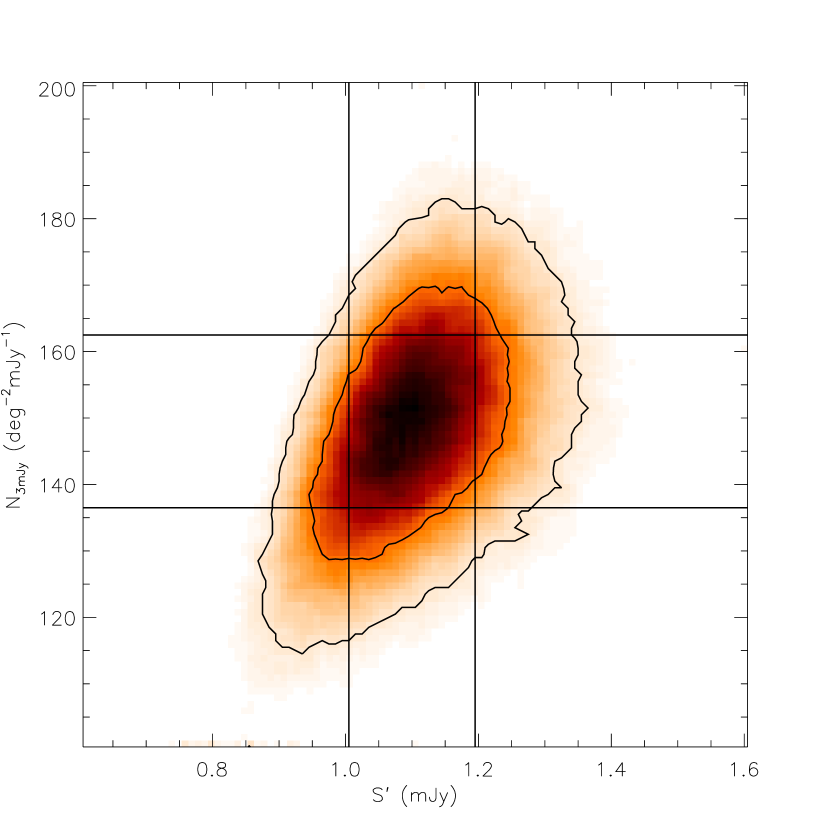
We avoid such complications in the derivation of best-fit statistics by implementing a bootstrap sampling method of parameter uncertainty estimation that is similar to what is used in the error estimation for the individual number count data points (Section 4.1). In this method, parameter space is explored by calculating best-fit parameters for each of the 100,000 number count bootstrap iterations. Fig. 10 shows the resulting parameter space for a two-parameter fit to the AzTEC/SHADES results using Equation 2 with Schechter parameter $\alpha$ fixed to a value of $-2$. Marginalised 68 per cent confidence intervals are used for the parameter uncertainties presented in Table 5. . We find that this alternative approach gives results that are comparable to that of formal fits, while providing a better characterisation of the true parameter probability distributions by avoiding assumptions of Gaussian distributed uncertainty in the fitted parameter and number count errors. Since an explicit flux value is chosen for each source upon an individual iteration of the bootstrap (i.e. a single flux is chosen from the source’s PFD), the number counts found by each realisation have flux bins that are effectively independent; therefore, this method provides a direct exploration of parameter space without necessitating an explicit calculation of the bin-to-bin correlations that exist amongst the final averaged results of Table 4.

Figure 10: Example distribution of best fit results of each iteration of bootstrapped AzTEC/SHADES number counts. Fits are to Equation 2 with the Schechter parameter $\alpha$ fixed to $-2$. Contours represent the 68 and 95 per cent confidence regions. Vertical and horizontal lines represent the marginalised 68 per cent confidence intervals of $S^{\prime}$ and $N_{\textrm{3mJy}}$, respectively.

Table 5: Parametric fits to differential number counts of Table 4 using Equation 2. Uncertainties of AzTEC-only fits represent the marginalised 68 per cent confidence intervals derived from the distribution of bootstrap iterations (Section 4.3). The Schechter parameter $\alpha$ is given in Column 4, and is held constant for fit results given without a confidence interval. The quantity $\alpha_{\textrm{dust}}$ is a free parameter representing the spectral index inferred by the simultaneous fit of the AzTEC/SHADES (1100–$\micron$) and SCUBA/SHADES (850–$\micron$) results, as described in the text. Uncertainties of the combined AzTEC and SCUBA fit are the formal 1$\sigma$ parameter errors when using Levenberg-Marquardt minimisation. The additional negative correction listed for $\alpha_{\textrm{dust}}$ represents an estimated correction for the systematic error induced by the SCUBA/SHADES choice of prior, as described in the text. All parameter values are for number counts at 1100–$\micron$.

Data Set	$S^{\prime}$	$N_{\textrm{3mJy}}$	$\alpha$	$\alpha_{\textrm{dust}}$
	(mJy)	($\textrm{deg}^{-2}\textrm{mJy}^{-1}$)
AzTEC/SHADES	$1.11^{+0.09}_{-0.09}$	$153^{+9}_{-17}$	$-2$	–
AzTEC/SHADES	$1.03^{+0.11}_{-0.43}$	$158^{+16}_{-21}$	$-1.8^{+1.1}_{-0.6}$	–
AzTEC/SHADES $+$ AzTEC/GOODS-N	$0.96^{+0.25}_{-0.33}$	$170^{+15}_{-20}$	$-1.56^{+0.65}_{-0.9}$	–
Two-Frequency Fits
AzTEC/SHADES + SCUBA/SHADES	$1.15\pm 0.07$	$153\pm 12$	$-2$	$(3.81-0.24)\pm 0.17$
AzTEC/SHADES + SCUBA/SHADES	$1.04\pm 0.21$	$157\pm 15$	$-1.75\pm 0.48$	$(3.83-0.25)\pm 0.17$

Table 5 also includes the results of simultaneous fits to the AzTEC/SHADES and published SCUBA/SHADES (Coppin et al., 2006) results, where we have assumed the two surveys are sampling the same source population and that the number counts of the two bands are consistent within an average scaling of flux density. These fits are accomplished through the introduction of a free spectral index parameter, $\alpha_{\textrm{dust}}$, which we have defined to reflect the average flux ratio between the two observing bands through the relation

$${S_{850}\over S_{1100}}=\left({\lambda_{850}\over\lambda_{1100}}\right)^{-\alpha_{\text{dust}}},$$ (4)

where $\lambda_{850}$ and $\lambda_{1100}$ represent the effective centre wavelengths of AzTEC and SCUBA, respectively (see also Perera et al., 2008). The combined SHADES fit, assuming the nominal band centres of 850 $\micron$ and 1100 $\micron$ and using Levenberg-Marquardt minimisation, gives $\alpha_{\textrm{dust}}=3.81\pm 0.17$ ($S_{850}/S_{1100}=2.67\pm 0.12$). The quoted uncertainties do not include systematic errors due to spectral differences between the SMGs and flux calibrators, which is expected to be smaller than the formal 1$\sigma$ uncertainty given, or any systematic calibration errors between the data sets (the 1$\sigma$ uncertainty of the formal fit is equivalent in size to a $\sim$5 per cent systematic error in the measured flux ratios). For optically thin thermal dust emission in the Rayleigh-Jeans limit ($\lambda\gg hc/kT$), $\alpha_{\text{dust}}$ represents the dust emissivity index ($\alpha_{\text{dust}}=2+\beta$); however, the Rayleigh-Jeans approximation is not strictly applicable at these wavelengths due to the expected temperature ($T_{\textrm{d}}\sim 35$ K; e.g. Chapman et al., 2005; Kovács et al., 2006; Coppin et al., 2008) and redshift ($\langle z\rangle\sim 2.2$; e.g. Chapman et al., 2005) of the typical SMG.

We have tested for various other systematics between the two instruments’ data sets by recalculating the AzTEC number counts under conditions and assumptions closely matching those existing for the SCUBA/SHADES analysis (Coppin et al., 2006). Since the AzTEC/SHADES survey includes additional mapped area not covered by SCUBA, the comparison of the two surveys may be susceptible to cosmic variance on large scales (i.e. $\mathrel{\lower 2.5pt\vbox{\hbox{$>$}\hbox{$\sim$}}}0.1\,$deg²). However, we find that there are no significant differences in the results when restricting the AzTEC analysis to only those regions covered by SCUBA. We also find no significant differences when applying the same 5 per cent null-threshold (Section 4.1) used in the SCUBA/SHADES analysis. The SCUBA analysis lacks a correction for the bias to peak map locations (Section 3.5), however, their use of the conservative 5 per cent null-threshold should keep this bias relatively small and it is expected to have no significant effect on the resultant number counts.

Finally, we note that the SCUBA analysis uses an external Bayesian prior that was based on 850–$\micron$ results of the Hubble Deep Field North (Borys et al., 2003), as opposed to the self-consistent iterative prior used in this paper. This prior represents a slight overabundance of bright SMGs when compared to the SCUBA/SHADES number counts, probably resulting in a small, but systematic, overestimate of the SCUBA/SHADES counts. Although we cannot use the exact same prior as SCUBA without inherently assuming an 850 $\micron$/1100 $\micron$ scaling relation (e.g. a value of $\alpha_{\textrm{dust}}$), we can adopt a similar prior that assumes the results of an 1100–$\micron$ survey of the same approximate field (AzTEC/GOODS-N; Perera et al., 2008). We recalculate the AzTEC/SHADES counts with this prior, as well as other matched systematics (5 per cent null-threshold, no correction for peak bias) to re-estimate $\alpha_{\textrm{dust}}$. These values are compared to the previous fits to determine the systematic error estimates given in Table 5 and result in a final corrected scaling index of $\alpha_{\textrm{dust}}\approx 3.6\pm 0.2$. As discussed in Section 5, this value of $\alpha_{\textrm{dust}}$ is significantly larger than that inferred by current measurements of the SMG redshift distribution (Chapman et al., 2005) and the SEDs of local starbursts (Dunne & Eales, 2001), as well as direct measurements of SMG flux ratios (Kovács et al., 2006; Coppin et al., 2008; Greve et al., 2008; Chapin et al., 2009). The lower $S_{850}/S_{1100}$ flux ratios detected through a direct comparison of SMGs detected in the GOODS-N field by both AzTEC and SCUBA (Chapin et al., 2009) indicate that our relatively high inferred flux ratio may be limited to the comparison of number counts and not due to systematic calibration errors between the two instruments. This suggests that the differences between the AzTEC and SCUBA number counts analyses and/or our assumptions of the source population (i.e. uniform flux ratio and the two wavebands track the same SMG population) lead to significant systematic errors in the inferred flux ratio at this level of sensitivity. Analysis of the 850$\micron$/1100$\micron$ flux density ratios of individual SHADES sources is deferred to Negrello et al. (in prep.).

5 Discussion

5.1 Comparison of 1.1 mm surveys

To appreciate the contribution of AzTEC/SHADES to our understanding of the SMG population, it must be compared to previous SMG surveys. The AzTEC/SHADES integral number counts are in strong disagreement with the parametric results derived from a fluctuation analysis of the 1.1–mm BOLOCAM Lockman Hole survey (dashed line in Fig. 8, Maloney et al., 2005). The BOLOCAM survey is significantly smaller and shallower than this AzTEC/SHADES survey and consequently contains fewer sources and is more susceptible to sample variance. Furthermore, the BOLOCAM fluctuation analysis is likely to be skewed by their requirement that the source population be well described by a single power law, which diverges at zero flux and has since been shown to poorly describe the SMG population over a wide range of flux densities (e.g. Scott et al., 2006; Coppin et al., 2006; this data set). Therefore, the BOLOCAM/LH single power-law result may represent a compromise between the relatively steep drop in SMG number counts at high flux density and the inevitably more moderate slope at the faint end.

Fig. 8 also shows the integral number counts for the individual AzTEC/LH (filled circles) and AzTEC/SXDF (open circles) fields at specific flux density limits. The two fields’ number counts are consistent within their respective uncertainties; however, the overall trend suggests that the AzTEC/LH field is rich in bright ($S_{1100}\mathrel{\lower 2.5pt\vbox{\hbox{$>$}\hbox{$\sim$}}}4$ mJy) sources relative to AzTEC/SXDF. This difference of bright AzTEC source counts is consistent with the differences seen between the regions of LH and SXDF surveyed by SCUBA at 850 $\micron$ (Coppin et al., 2006).

The effects of cosmic variance appear more prevalent when comparing the results of this survey to the $0.15$ deg² AzTEC/COSMOS survey (Scott et al., 2008), which targeted a region with significant structure, as traced by the optical/IR galaxy population at $z\mathrel{\lower 2.5pt\vbox{\hbox{$<$}\hbox{$\sim$}}}1.1$ (Scoville et al., 2007). The average blank-field number counts of AzTEC/SHADES confirm the significant over-density of bright 1.1–mm sources in the AzTEC/COSMOS region first reported in Austermann et al. (2009), who conclude that the observed over-density is probably due to gravitational lensing by foreground ($z\mathrel{\lower 2.5pt\vbox{\hbox{$<$}\hbox{$\sim$}}}1.1$) structure (comparisons between SHADES sources and other populations/structure will be explored in future SHADES papers). We have recalculated the AzTEC/COSMOS number counts using the AzTEC/SHADES prior and a 20 per cent null-threshold (Fig. 8), affirming that the AzTEC/COSMOS over-density is significant regardless of the chosen prior.

We similarly find that the AzTEC/GOODS-N region is relatively rich in 1.1–mm sources compared to the much larger AzTEC/SHADES survey. This is consistent with the relative abundances found in the comparable 850–$\micron$ surveys of GOODS-N (Borys et al., 2003) and SHADES (Coppin et al., 2006). The higher number counts of AzTEC/GOODS-N may be due to sample and/or cosmic variance on the scale of the GOODS-N map (0.068 deg² to $\sim 1$ mJy), which can be exemplified by moving a box the size of AzTEC/GOODS-N to different locations within the well-covered, and similar depth, regions of the AzTEC/LH map (e.g. dash-dotted rectangle in Fig. 2(a)). This simple exercise shows that the total number of source candidates within the GOODS-N sized box can change by a factor of $\sim$ 2 for any of the source definitions explored here (i.e. null-threshold 5–20 per cent). The relatively high number of bright SMGs found in GOODS-N may be due, in part, to potential high-redshift structures in the GOODS-N field (Chapman et al., 2009; Daddi et al., 2009).

To better quantify the empirical variations across fields, we turn to the formalism of Efstathiou et al. (1990). Taking the three ‘blank-fields’ considered here (AzTEC/LH, AzTEC/SXDF, AzTEC/GOODS-N) as independent ‘cells’ and using Equations 9 & 5 from Efstathiou et al. (1990), we can calculate $\sigma^{2}$ and $\textrm{Var}(\sigma^{2})$, where $\sigma^{2}$ is defined by Equation 1b of the same paper and represents the variation from cell to cell, or in this case field to field. The variations in field size and completeness are taken into account as per the ‘counts in cells’ formalism of Efstathiou (1990). For $\textrm{Var}(\sigma^{2})$ we assume zero variance ($\sigma^{2}=0$) such that the significance of the measurement is essentially the ‘detection’ significance of some field to field variation.

Number count data at the lowest fluxes, $S_{1100}<2$ mJy, are omitted from this analysis due to their sensitivity to the assumed Bayesian prior, which is held constant for all fields (Section 4). Any bias to the prior would result in measured field-to-field variations that are systematically lower than that expected from Poisson statistics. This bias is relatively small for the remaining data ($S_{1100}>2$ mJy) and, to the extent that it is present, would act to make the fields’ measured number counts systematically less varied and our empirical variance measurements conservatively low. We combine the counts such that we test the variations in two relatively well-sampled flux bins: 2–4 mJy, and $>4$ mJy.

Table 6 contains the results of this variance analysis. For the AzTEC ‘blank-fields’ alone, no significant detection of variance is found. The 2–4 mJy flux bin has a $\sigma^{2}$ that is strongly negative, indicating that the measured variance of that bin is significantly less than that expected from Poisson statistics, while the $>4$ mJy flux bin has a variance consistent with $\sigma^{2}=0$. The former may be a consequence of the fact that AzTEC/LH and AzTEC/SXDF have coincidentally similar number counts compared to their formal uncertainty in the 2–4 mJy range.

The results when including the AzTEC/COSMOS data as an additional cell in the analysis are also given in Table 6. It can be seen that for the brightest sources $S_{1100}>4$ mJy some variance is detected at the 3.8$\sigma$ level. This further confirms the significant over-density of bright 1.1–mm sources in the AzTEC/COSMOS region.

Table 6: Statistical significance of the variations in the number counts between the three fields considered here (LH, SXDF, GOODS-N), as well as the COSMOS field

Flux	$\sigma^{2}$	$\Delta(\sigma^{2})$	Significance	N′
(mJy)			$\left(\frac{\sigma^{2}}{\Delta\sigma^{2}}\right)$	($deg^{-2}$)
LH, SXDF, GOODS-N only
2–4	$-8.9\times 10^{-3}$	2.3$\times 10^{-2}$	–	464.5
$>4$	7.9$\times 10^{-2}$	8.2$\times 10^{-2}$	0.96	50.3
LH, SXDF, GOODS-N and COSMOS
2–4	1.1$\times 10^{-2}$	2.3$\times 10^{-2}$	0.48	489.9
$>4$	2.4$\times 10^{-1}$	6.4$\times 10^{-2}$	3.8	62.2

Notes: Negative $\sigma^{2}$ indicates the measured variance is less than expected from Poisson statistics.

Interestingly, with the exception of the $>4$ mJy sources across all 4 fields, these results are fairly consistent with what would be expected from consideration of the expected form of the correlation function. The expected variance can be calculated by integration of the correlation function

$$\sigma^{2}=\int\int_{V}\xi(r)\,dV\,dV,$$

where the integral is calculated over a volume, $V$, defined as a truncated cone of solid angle $\Omega$ over the redshift range $2<z<3$. We assume a correlation function of the form $\xi(r)=(r/r_{0})^{-\gamma}$, with $r_{0}=5h^{-1}{\rm Mpc}$ and $\gamma=1.8$, which are typical for local galaxy populations. Assuming field sizes in the range 0.07–0.37 deg². gives a predicted variance of between 0.017 and 0.008, respectively. The measured variance for the number density of $S_{1100}>4$ mJy sources across all 4 fields is in significant excess of that predicted under the above assumptions.

However it is worth noting that the quoted errors on the measured $\sigma^{2}$ assume no clustering, and are therefore underestimates of the true measurement error. In addition it is known that the COSMOS field contains a significant over-density of 1.1–mm sources (Austermann et al., 2009). Taken together it is clear that the COSMOS field is simply a highly unusual example, and the volumes probed by these surveys are not great enough to detect a clustering signal of bright SMGs through the comparison of number counts alone.

5.2 Comparison to 850–$\micron$ counts

As shown in Fig. 8, the SCUBA 850–$\micron$ and AzTEC 1100–$\micron$ SHADES counts are consistent within a uniform scaling of flux density (Section 4.3). Under the assumption that AzTEC and SCUBA are sampling the same source population (ignoring selection effects), $\alpha_{\textrm{dust}}$ represents a power law approximation to the average redshifted SMG SED at observed wavelengths of $\sim 1$ mm. The relatively steep 850 $\micron$/1100 $\micron$ spectral index derived from the SMG populations of SHADES (after an approximate correction of systematics due to chosen priors; see Section 4.3), $\alpha_{\textrm{dust}}\approx 3.6\pm 0.2$, is roughly consistent with the 450 $\micron$/850 $\micron$ spectral index, $\alpha_{\textrm{dust}}\approx$ 3.6–3.7, found by the SCUBA Local Universe Galaxy Survey (SLUGS) of IR bright galaxies in the local Universe (Dunne & Eales, 2001) after correcting for an average CO(3–2) contamination of 25 per cent in the 850–$\micron$ band at $z=0$ (Seaquist et al., 2004). However, the 450 $\micron$ measurements from SLUGS are already shortward of the Rayleigh-Jeans limit (but longward of the peak) in the local Universe; particularly as local galaxy SEDs require two or more dust temperature components, with the cooler component being $\sim 20$ K. For a population of SMGs residing at the typical redshift of $z\sim 2$, the observed 850–$\micron$ SCUBA band is sampling a rest-frame wavelength of $\sim$ 280 $\micron$. To produce a similar $\alpha_{\textrm{dust}}$ to the SLUGS galaxies in the local Universe, a much hotter temperature is required for the SED ($T\geq 50$ K with $\beta=2$). Alternatively, these SMGs could have similar SEDs to the local galaxies but reside at lower redshifts ($z\mathrel{\lower 2.5pt\vbox{\hbox{$<$}\hbox{$\sim$}}}1$), although this would be inconsistent with measured SMG redshift distributions (Chapman et al., 2005). The inferred sub-mm/mm flux ratio is high compared to the model predictions of Swinbank et al. (2008) and at odds with measurements of the flux ratios $S_{350}/S_{850}$ (Kovács et al., 2006; Coppin et al., 2008), $S_{850}/S_{1100}$ (Chapin et al., 2009), and $S_{850}/S_{1200}$ (Greve et al., 2008), which are all more consistent with the SLUGS SEDs for $z\sim 2$. In addition, the existence of a population of sub-millimetre drop-outs (SDOs; e.g. Greve et al., 2008) – sources with a combination of high-redshift and/or low dust temperature such that the 850–$\micron$ band samples near, or shortward, of the peak emission – would act to lower the average value $\alpha_{\textrm{dust}}$ for millimetre detected sources.

It thus appears that our estimate of $\alpha_{\textrm{dust}}$ is systematically large given the expectation that $\beta\mathrel{\lower 2.5pt\vbox{\hbox{$<$}\hbox{$\sim$}}}2$ (Dunne & Eales, 2001, and references therein) and that the majority of our sources are unlikely to be fully in the Rayleigh-Jeans limit. This bias may be indicative of further systematics in the SCUBA/SHADES choice of prior (Section 4.3), potentially insufficient de-boosting of low $S/N$ SCUBA detections (as suggested in a direct comparison of sources detected by both AzTEC and SCUBA in the GOODS-N field; Chapin et al., 2009), or that selection bias somehow results in a systematic increase in the value of $\alpha_{\textrm{dust}}$ inferred from SMG number counts when assuming 850 $\micron$ and 1100 $\micron$ sample the same approximate source population. A straight comparison of the AzTEC and SCUBA SHADES maps (Negrello et al., in prep.) will provide a more direct measure of $\alpha_{\textrm{dust}}$ that is based on individual sources and fluxes in the maps and search for evidence of SDOs in the SHADES fields.

5.3 Predictions from models

Finally, we compare the AzTEC/SHADES number counts to those predicted at 1100 $\micron$ by various IR/sub-mm formation and evolution models in figs. 7 and 8. The predictions of the IR/sub-mm evolution models of Rowan-Robinson (2009) are shown for high-redshift formation limits of $z_{\textrm{f}}=4$ and $z_{\textrm{f}}=5$. The AzTEC/SHADES number counts agree with the $z_{\textrm{f}}=4$ model at fluxes $S_{1100}\mathrel{\lower 2.5pt\vbox{\hbox{$<$}\hbox{$\sim$}}}4$ mJy, but are systematically lower than the predictions at higher fluxes. A semi-analytical model for the joint formation and evolution of spheroids and QSOs (Granato et al., 2004; Silva et al., 2005) predicts very similar number counts at 1100 $\micron$. These models are in better overall agreement with the high flux number counts seen in the AzTEC/COSMOS and AzTEC/GOODS-N fields; however, those fields have significant biases and/or limitations, as discussed above. Also compared are the counts predicted by the semi-analytical galaxy formation model of Baugh et al. (2005, see also , ), which systematically over-predicts the number of sources seen in AzTEC/SHADES by a factor of 3–4 at all measured fluxes. Finally, we compare our results to the early predictions for SHADES (van Kampen et al., 2005) – models constrained to the SCUBA 8-mJy (i.e. $S_{1100}\geq 3$ mJy) survey (Scott et al., 2002) – which forecast a shallower slope in the number counts than seen in the AzTEC/SHADES fields. Assuming the bright sources are uniformly distributed across the sky, the AzTEC/SHADES survey suggests that all of these models significantly over-predict the number of intrinsically bright SMGs. If, instead, these relatively rare sources are strongly clustered, the true all-sky average number density of the brightest SMGs could be higher (or lower) than indicated by this survey, potentially bridging the gap between model and observation.

6 Conclusions

AzTEC/SHADES is the largest extragalactic millimetre-wave survey to date, with over 0.7 deg² mapped to depths of $0.9<\sigma_{1.1}<1.7$ mJy. This survey, split between the Subaru/XMM-Newton Deep Field and the Lockman Hole, provides over 100 significant individual detections at 1.1 mm, with most representing newly discovered mm-wave sources. These maps also provide information on the fainter SMG population through the signature of numerous dimmer sources that are partially buried in the noise.

Combined with our improved methods for number count estimates, AzTEC/SHADES provides the tightest available constraints on the average SMG population in the flux range $1$ mJy $\mathrel{\lower 2.5pt\vbox{\hbox{$<$}\hbox{$\sim$}}}S_{1100}\mathrel{\lower 2.5pt\vbox{\hbox{$<$}\hbox{$\sim$}}}10$ mJy. In particular, the AzTEC/SHADES results represent a significant advance in our knowledge of the blank-field population at 1.1 mm, showing that there are significantly lower densities of bright SMGs than that suggested by smaller 1.1–mm surveys published previously. An accurate understanding of the average SMG population is critical for comparisons to source counts found in biased and/or over-dense regions. The AzTEC/SHADES blank-field counts confirm the over-density of $S_{1100}>2$ mJy sources found in the AzTEC/COSMOS field (Austermann et al., 2009) and show that the GOODS-N field is also relatively rich in bright SMGs, thus suggesting that cosmic variance can significantly affect the observed number density of SMGs in mass-biased regions (AzTEC/COSMOS) and/or on relatively small scales (AzTEC/GOODS-N; $0.068$ deg²). We find that the variance in number counts seen across the four available AzTEC/JCMT survey fields (LH, SXDF, COSMOS, GOODS-N) is significantly larger than that expected from Poisson statistics alone, particularly at $S_{1100}>4$ mJy, thus suggesting that bright SMGs may be strongly clustered.

The AzTEC/SHADES results are consistent with the predictions of the formation and evolution models of Granato et al. (2004) and the $z_{\textrm{f}}\sim 4$ evolution models of Rowan-Robinson (2009) for blank-field 1.1–mm source counts at $S_{1100}\mathrel{\lower 2.5pt\vbox{\hbox{$<$}\hbox{$\sim$}}}4$ mJy; however, these models systematically over-predict the number of AzTEC/SHADES sources seen at higher fluxes, although the relative scarcity and potential clustering of bright sources leaves even this unprecedentedly large SMG survey susceptible to the effects of cosmic variance. A truly unambiguous characterisation of the $S_{1100}\mathrel{\lower 2.5pt\vbox{\hbox{$>$}\hbox{$\sim$}}}6$ mJy SMG population will require significantly larger-area surveys at (sub-)mm wavelengths, such as those expected to be conducted in the coming year(s) by SCUBA-2 on the JCMT and AzTEC when mounted on the Large Millimeter Telescope (LMT).

We find that the SCUBA/SHADES and AzTEC/SHADES number counts are consistent within a uniform scaling of flux density. Assuming that the 850 $\micron$ and 1100 $\micron$ wavebands sample the same underlying source population, this scaling corresponds to an average source flux ratio of $S_{850}/S_{1100}\approx 2.5\pm 0.1$, once corrected for known systematics between the data sets. This ratio is significantly larger than that expected for the high-redshift SMG population and we find that the systematics induced by small differences in the number count analyses of the two surveys and the assumption of a uniformly scalable flux density limit the robustness of the inferred flux ratio. The S850/S1100 flux ratio is explored further in a direct comparison of individual sources lying in the overlapping regions of the SCUBA and AzTEC surveys (Negrello et al., in prep.).

Appendix A Correlation Matrix

The bootstrap sampling method of Section 4.1 induces significant correlation between the final averaged differential number count bins (e.g. Table 4) through discrete sampling (and consequent binning) of continuous PFDs that have significant probability on scales comparable to, or larger than, the bin size (1 mJy in this paper). Previous incarnations of this sampling method (e.g. Coppin et al., 2006) estimated covariance and correlation matrices directly from the variation in number count results seen across the iterations of the bootstrap. This sampling method collapses each source’s probability distribution (PFD; e.g. Fig. 4) to a single flux upon each iteration, which acts to hide significant correlation amongst the final binned results by throwing away much of the cross-bin information contained within the PFD. This resulted in severely underestimated bin-to-bin correlations amongst the differential number counts data, as was evidenced by the unrealistically low $\chi^{2}$ values of formal fitting (Coppin et al., 2006; Perera et al., 2008; Austermann et al., 2009).

Table 7: Correlation matrix of the AzTEC/SHADES differential count bins as given in Table 4. The last row gives the standard deviation of each bin as determined through the bootstrap sampling method of Section 4.1. Together, these values can be used to create a covariance matrix; however, we note that the probability distribution is not strictly Gaussian, particularly for the less populated bins, as evidenced by the asymmetric uncertainty intervals of Table 4.

FLUX	1.38	2.40	3.40	4.41	5.41	6.41	7.41
(mJy)
1.38	1.00	0.92	0.61	0.26	0.08	0.02	0.01
2.40	0.92	1.00	0.84	0.47	0.18	0.04	0.01
3.40	0.61	0.84	1.00	0.82	0.44	0.12	0.05
4.41	0.26	0.47	0.82	1.00	0.78	0.32	0.17
5.41	0.08	0.18	0.44	0.78	1.00	0.77	0.61
6.41	0.02	0.04	0.12	0.32	0.77	1.00	0.97
7.41	0.01	0.01	0.05	0.17	0.61	0.97	1.00
$\sigma$	179.77	46.40	16.69	7.55	3.98	2.38	1.33

We now present an alternative method of calculating the correlation matrix which better captures these correlations amongst the final differential number count bins. We begin by integrating the PFD of each source over the span of each flux bin. These binned probabilities can be summed over all sources to provide a number counts estimate that matches the final averaged results of the full bootstrapping method, but without the robust uncertainty estimates that the bootstrap method is designed to provide. We apply this alternative number counts estimate to each of the 100,000 unique catalogues produced by the bootstrap. The Poisson deviation and replacement sampling used to produce each catalogue (Section 4.1) act to perturb this new estimate of the number counts around the most likely values. This collection of perturbed number counts is then used to estimate the correlation between the differential number count bins.

We present the resulting correlation matrix for the AzTEC/SHADES differential results (Section 4) in Table 7. These correlations apply directly to the differential results provided in Table 4 and Fig. 7 (20 per cent threshold counts). The last row of Table 7 provides the standard deviation of the differential counts of each flux bin, as estimated in the bootstrap sampling method. These values can be applied to the correlation matrix to produce a covariance matrix for the data. However, the standard deviation is not an ideal representation of the true uncertainty distribution (Table 4) due to the finite sampling of each bin, which results in an asymmetric multinomial probability distribution (i.e. non-Gaussian). As discussed in Section 4.3, care must be taken when attempting to use this covariance matrix in typical fitting algorithms due to the high level of degeneracy amongst the bins. Larger flux bins could be used to reduce the bin-to-bin correlations; however, significantly larger bins would make flux resolution the limiting factor (with respect to the precision of the AzTEC/SHADES differential number counts estimate) for most practical applications of the data.

References

- Alexander et al. (2005) Alexander, D. M., Bauer, F. E., Chapman, S. C., Smail, I., Blain, A. W., Brandt, W. N., & Ivison, R. J. 2005, ApJ, 632, 736
- Aretxaga et al. (2007) Aretxaga, I., et al. 2007, MNRAS, 379, 1571
- Austermann et al. (2009) Austermann, J. E., et al. 2009, MNRAS, 123
- Barger et al. (1998) Barger, A. J., Cowie, L. L., Sanders, D. B., Fulton, E., Taniguchi, Y., Sato, Y., Kawara, K., & Okuda, H. 1998, Nature, 394, 248
- Baugh et al. (2005) Baugh, C. M., Lacey, C. G., Frenk, C. S., Granato, G. L., Silva, L., Bressan, A., Benson, A. J., & Cole, S. 2005, MNRAS, 356, 1191
- Bertoldi et al. (2007) Bertoldi, F., et al. 2007, ApJS, 172, 132
- Biggs & Ivison (2006) Biggs, A. D., & Ivison, R. J. 2006, MNRAS, 371, 963
- Blain et al. (2002) Blain, A. W., Smail, I., Ivison, R. J., Kneib, J.-P., & Frayer, D. T. 2002, Phys. Rep., 369, 111
- Blain et al. (2004) Blain, A. W., Chapman, S. C., Smail, I., & Ivison, R. 2004, ApJ, 611, 725
- Borys et al. (2003) Borys, C., Chapman, S., Halpern, M., & Scott, D. 2003, MNRAS, 344, 385
- Chapman et al. (2003) Chapman, S. C., Windhorst, R., Odewahn, S., Yan, H., & Conselice, C. 2003, ApJ, 599, 92
- Chapman et al. (2005) Chapman, S. C., Blain, A. W., Smail, I., & Ivison, R. J. 2005, ApJ, 622, 772
- Chapman et al. (2009) Chapman, S. C., Blain, A., Ibata, R., Ivison, R. J., Smail, I., & Morrison, G. 2009, ApJ, 691, 560
- Chapin et al. (2009) Chapin, E. L., et al. 2009, arXiv:0906.4561
- Clements et al. (2008) Clements, D. L., et al. 2008, MNRAS, 387, 247
- Coppin et al. (2005) Coppin, K., Halpern, M., Scott, D., Borys, C., & Chapman, S. 2005, MNRAS, 357, 1022
- Coppin et al. (2006) Coppin, K., et al. 2006, MNRAS, 372, 1621
- Coppin et al. (2008) Coppin, K., et al. 2008, MNRAS, 384, 1597
- Daddi et al. (2009) Daddi, E., et al. 2009, ApJ, 694, 1517
- Dunne & Eales (2001) Dunne, L., & Eales, S. A. 2001, MNRAS, 327, 697
- Dye et al. (2008) Dye, S., et al. 2008, MNRAS, 386, 1107
- Efstathiou et al. (1990) Efstathiou, G., Kaiser, N., Saunders, W., Lawrence, A., Rowan-Robinson, M., Ellis, R. S., & Frenk, C. S. 1990, MNRAS, 247, 10P
- Farrah et al. (2002) Farrah, D., Verma, A., Oliver, S., Rowan-Robinson, M., & McMahon, R. 2002, MNRAS, 329, 605
- Farrah et al. (2006) Farrah, D., et al. 2006, ApJ, 641, L17
- Granato et al. (2004) Granato, G. L., De Zotti, G., Silva, L., Bressan, A., & Danese, L. 2004, ApJ, 600, 580
- Greve et al. (2004) Greve, T. R., Ivison, R. J., Bertoldi, F., Stevens, J. A., Dunlop, J. S., Lutz, D., & Carilli, C. L. 2004, MNRAS, 354, 779
- Greve et al. (2007) Greve, T. R., Stern, D., Ivison, R. J., De Breuck, C., Kovács, A., & Bertoldi, F. 2007, MNRAS, 382, 48
- Greve et al. (2008) Greve, T. R., Pope, A., Scott, D., Ivison, R. J., Borys, C., Conselice, C. J., & Bertoldi, F. 2008, MNRAS, 389, 1489
- Greve et al. (2009) Greve, T. R., et al. 2009, arXiv:0904.0028
- Griffin & Orton (1993) Griffin, M. J., & Orton, G. S. 1993, Icarus, 105, 537
- Hogg & Turner (1998) Hogg, D. W., & Turner, E. L. 1998, PASP, 110, 727
- Hogg (2001) Hogg, D. W. 2001, AJ, 121, 1207
- Holland et al. (2006) Holland, W., et al. 2006, SPIE, 6275, 45
- Hughes et al. (1998) Hughes, D. H., et al. 1998, Nature, 394, 241
- Ibar et al. (2009) Ibar, E., Ivison, R. J., Biggs, A. D., Lal, D. V., Best, P. N., & Green, D. A. 2009, arXiv:0903.3600
- Ivison et al. (2007) Ivison, R. J., et al. 2007, MNRAS, 380, 199
- Kovács et al. (2006) Kovács, A., Chapman, S. C., Dowell, C. D., Blain, A. W., Ivison, R. J., Smail, I., & Phillips, T. G. 2006, ApJ, 650, 592
- Lacey et al. (2008) Lacey, C. G., Baugh, C. M., Frenk, C. S., Silva, L., Granato, G. L., & Bressan, A. 2008, MNRAS, 385, 1155
- Laurent et al. (2005) Laurent, G. T., et al. 2005, ApJ, 623, 742
- Lonsdale et al. (2006) Lonsdale, C. J., Farrah, D., & Smith, H. E. 2006, Astrophysics Update 2, 285
- Magliocchetti et al. (2007) Magliocchetti, M., Silva, L., Lapi, A., de Zotti, G., Granato, G. L., Fadda, D., & Danese, L. 2007, MNRAS, 375, 1121
- Maloney et al. (2005) Maloney, P. R., et al. 2005, ApJ, 635, 1044
- Menéndez-Delmestre et al. (2007) Menéndez-Delmestre, K., et al. 2007, ApJ, 655, L65
- Mortier et al. (2005) Mortier, A. M. J., et al. 2005, MNRAS, 363, 563
- Perera et al. (2008) Perera, T. A., et al. 2008, MNRAS, 391, 1227
- Pope et al. (2006) Pope, A., et al. 2006, MNRAS, 370, 1185
- Pope et al. (2008) Pope, A., et al. 2008, ApJ, 675, 1171
- Press et al. (1992) Press, W. H., Teukolsky, S. A., Vetterling, W. T., & Flannery, B. P. 1992, Cambridge: University Press, —c1992, 2nd ed.,
- Priddey et al. (2008) Priddey, R. S., Ivison, R. J., & Isaak, K. G. 2008, MNRAS, 383, 289
- Rowan-Robinson (2009) Rowan-Robinson, M. 2009, MNRAS, 394, 117
- Scott et al. (2002) Scott, S. E., et al. 2002, MNRAS, 331, 817
- Scott et al. (2006) Scott, S. E., Dunlop, J. S., & Serjeant, S. 2006, MNRAS, 370, 1057
- Scott et al. (2008) Scott, K. S., et al. 2008, MNRAS, 385, 2225
- Scoville et al. (2007) Scoville, N., et al. 2007, ApJS, 172, 150
- Seaquist et al. (2004) Seaquist, E., Yao, L., Dunne, L., & Cameron, H. 2004, MNRAS, 349, 1428
- Serjeant et al. (2008) Serjeant, S., et al. 2008, MNRAS, 386, 1907
- Silva et al. (2005) Silva, L., De Zotti, G., Granato, G. L., Maiolino, R., & Danese, L. 2005, MNRAS, 357, 1295
- Simpson et al. (2006) Simpson, C., et al. 2006, MNRAS, 372, 741
- Smail et al. (1997) Smail, I., Ivison, R. J., & Blain, A. W. 1997, ApJ, 490, L5
- Stevens et al. (2003) Stevens, J. A., et al. 2003, Nature, 425, 264
- Swinbank et al. (2008) Swinbank, A. M., et al. 2008, MNRAS, 391, 420
- Tamura et al. (2009) Tamura, Y., et al. 2009, Nature, 459, 61
- van Kampen et al. (2005) van Kampen, E., et al. 2005, MNRAS, 359, 469
- Wilson et al. (2008) Wilson, G. W., et al. 2008, MNRAS, 386, 807