Channel coupling in heavy quarkonia: energy levels, mixing, widths and new states
Abstract
The mechanism of channel coupling via decay products is used to study energy shifts, level mixing as well as the possibility of new near-threshold resonances in systems. The Weinberg eigenvalue method is formulated in the multichannel problems, which allows to describe coupled-channel resonances and wave functions in a unitary way, and to predict new states due to channel coupling. Realistic wave functions for all single-channel states and decay matrix elements computed earlier are exploited, and no new fitting parameters are involved. Examples of level shifts, widths and mixings are presented; the dynamical origin of and the destiny of the single-channel state are clarified. As a result a sharp and narrow peak in the state with quantum numbers is found at 3.872 GeV, while the single-channel resonance originally around 3.940 GeV, becomes increasingly broad and disappears with growing coupling to open channels.
pacs:
12.39.-x,13.20.Gd,13.25.Gv,14.40.GxI INTRODUCTION
Most hadron states are coupled by strong interaction to closed or open decay channels, and thus are subjects of the Theory of Strongly Coupled Channels (TSCC). The latter topic was developed during many decades, see Eichten et al. (1980); *Eichten:1978tg; *Eichten:1975ag; Geiger and Isgur (1993); *Geiger:1991qe; *Geiger:1991ab; *Geiger:1989yc; van Beveren et al. (1983); *vanBeveren:1979bd; Tornqvist (1995); *Tornqvist:1995ay and Badalian et al. (1982) for a review, and also Kalashnikova (2005); *Baru:2003qq; Barnes and Swanson (2008); Pennington and Wilson (2007) as more recent publications. In the present paper we apply TSCC specifically to the case of Okubo-Zweig-Iizuka rule allowed two-body decay channels of charmonia and bottomonia. In doing so we need several prerequisites. First of all, it is the one-channel description of charmonia and bottomonia as , states in relativistic Hamiltonian formalism Dubin et al. (1993); *Badalian:2008sv, developed in the framework of the Field Correlator method (FCM) Dosch (1987); *Dosch:1988ha; *Simonov:1987rn (see Di Giacomo et al. (2002) for a review) and wave functions of stable states in or space cast in the numerical form. The latter have been accurately computed using this method with only universal input: the string tension , the current (pole) quark masses , and the strong coupling Badalian and Danilkin (2009); *Badalian:2004gw; *Badalian:2008dv; *Badalian:2007zz.
The next ingredient is an effective relativistic Lagrangian for the pair creation, inducing the string breaking. To this end we are using the decay mass vertex introduced in Simonov (2008) and exploited for dipion transitions in Simonov (2008); Simonov and Veselov (2009a, b) and for the reaction channel in Simonov and Veselov (2008). In principle, can be expressed in terms of quark masses and average energies, but we use it as the only one parameter, which is fixed in our previous studies Simonov (2008); Simonov and Veselov (2009a, b); Simonov and Veselov (2008) Finally, as it was shown in Simonov (2008) and before in Barnes et al. (2005); *Barnes:1991em; Ackleh et al. (1996) the transition matrix element reduces to the overlap integral of wave functions of decaying system and products of decay. It is interesting, that the vertex operator in this integral contains not only , but also the factor of the decay process constructed from the Dirac trace of all involved hadron vertex states, and projection operators. This technic, introduced in Simonov (2008), is a relativistic equivalent of the nonrelativistic one with spin-angular momentum (Clebsch-Gordon) coefficients used in the framework of model Micu (1969); *LeYaouanc:1972ae; *LeYaouanc:1977ux; *LeYaouanc:1977gm. As a result one obtains a system of integrodifferential equations for new wave functions and energy eigenvalues, which can be easily solved in the lowest approximation for energy shifts, widths and level mixing coefficients. At the same time we have developed a variant of wave functions and matrix elements for light quarks in heavy-light mesons. Several examples of this kind are shown below.
At a deeper level, one meets with several problems: (i) First, the states above decay thresholds are unstable and the definition of the wave function itself is questionable in a rigorous sense, since an admixture of continuous spectrum states appears. Here different approaches exist. The most rigorous is the Weinberg procedure Weinberg (1963); *newton:319; *Smithies1958, named below the Weinberg Eigenvalue Method (WEM). It is used to define the resonance wave function and energy, as well as -matrix via Weinberg eigenvalues. The WEM has been used before in the one-channel 2-body and 3-body problems Weinberg (1963); *newton:319; *Smithies1958,Narodetsky (1981); *Narodetsky:1969jf; *Herzenberg; *Fuda. We have found that it is specifically useful in case of TSCC, since coupled channels (CC) induce the energy-dependent force term, which violates standard orthonormalization procedure, while this term can easily be treated in WEM. (ii) Second, even the closed channels cause the problems. In terms of hadron loops it was treated in many papers, see e.g. Geiger and Isgur (1993); *Geiger:1991qe; *Geiger:1991ab; *Geiger:1989yc and recent papers Barnes and Swanson (2008); Pennington and Wilson (2007), where some theorems were formulated Barnes and Swanson (2008) and the renormalization method was suggested Pennington and Wilson (2007).
In essence the problem here is similar to the problem of unquenched quark pairs. It occurs also for stable hadrons, where the renormalozation procedure is necessary in general. We will not discuss these topics in the given paper, assuming that the renormalization is done e.g., by readjusting the pole quark mass. We also disregard the important topic of full relativistic invariance for composite objects moving with different velocities, e.g. charmonium decaying in its c.m. system into heavy-light mesons, with their wave functions defined in their c.m. systems. This is done assuming small relative velocities near thresholds. Far from thresholds these factors become important. Similarly, near thresholds we assume here, as well as in Simonov (2008); Simonov and Veselov (2009a, b); Simonov and Veselov (2008), the type of the decay vertex, while at higher energies this type of decay may be replaced by another one, e.g. the type.
In this paper we systematically apply WEM to find the shifts and widths of energy levels, as well as mixing between them. We find the method to be especially useful to discover the analytic structure and pole positions in the case of strong CC. A particular example of the level proves to be a good illustration of our analysis. From the experimental point of view two interesting problems appear. First one, why in experiment only the peak at the lowest threshold is seen, while at the slightly higher, no peak was ever seen? Secondly, possible resonances at 3.940 GeV found in Abe et al. (2007); *Pakhlova:2008di; *Yuan:2009iu, seemingly are not , and very likely the state around 3.940 GeV was never observed. Our analysis allows to answer both questions at the same time, as will be explained below.
As a result we find two poles due to a single eigenvalue in the possitions near 3.872 GeV and 3.940 GeV, but the latter peak becomes too wide and finally disappears with increasing , which can explain the experimental situation Abe et al. (2007); *Pakhlova:2008di; *Yuan:2009iu. Moreover, retaining the peak appears at the lower threshold 3.872 GeV, and not at the higher threshold 3.879 GeV, again in agreement with experiment Abe et al. (2007); *Pakhlova:2008di; *Yuan:2009iu.
The plan of the paper is as follows. In the next section we introduce the general formalism for the Green’s functions of charmonia and bottomonia with the inclusion of decay channels. We present equations for wave functions (Green’s functions) both in and channels. In section III the CC resonances are considered in the decay channel and condition for the existence of a CC resonance is formulated. In section IV the rigorous Weinberg theory of CC resonances is presented. In section V the mixing of states in WEM is considered. In section VI we present results for values of level shifts and widths for state and also mixing between and state, as well as the analysis of the situation in the state. In section VII summary and prospectives are given.
II GENERAL FORMALISM OF STRING-BREAKING CHANNEL COUPLING
We consider two sectors of hidden and open flavor with initial and final bare gauge invariant operators, for heavy quarkonium sector,
I.
and for heavy-light meson sector,
II. ,
where With the help of one
generates bare mesons and as shown in
Simonov (2008); Badalian et al. (2007) one can project physical
amplitudes 111Note, that the procedure of hadron state
projection is here fully equivalent to that used in lattice
approach, see e.g.
Hashimoto et al. (1999); *Becirevic:2004ya; *Brommel:2007wn; *Bowler:1996ws.
(Green’s functions) with physical wave functions
. For stationary states one can use
Green’s functions in energy representation, e.g.
| (1) |
Here superscript (0) of Green’s function refers to the bare case, when sector II is switched off, and refer to the eigenfunctions and eigenvalues of the relativistic string Hamiltonian Dubin et al. (1993); *Badalian:2008sv, for charmonium those were calculated in Badalian and Danilkin (2009); *Badalian:2004gw; *Badalian:2008dv; *Badalian:2007zz and for bottomonium in Badalian et al. (2009b); *Badalian:2009bu; *Badalian:2004xv. In sector II the counterpart of (1) consists of Green’s function of the pair . We neglect in the first approximation interaction of two color singlet mesons, and write the c.m. Green’s function as
| (2) |
At this point we must take into account a possible transition (decay) of states in sector I into states of sector II, which can be done in several ways. In literature it is common to assume one of several types of phenomenological decay Lagrangians, e.g. type Micu (1969); *LeYaouanc:1972ae; *LeYaouanc:1977ux; *LeYaouanc:1977gm, with vector confinement vertex Eichten et al. (1980); *Eichten:1978tg; *Eichten:1975ag, or with scalar confinement vertex, studied in Ackleh et al. (1996). For bottomonium a relativistic string decay vertex of the following form was used in Simonov (2008); Simonov and Veselov (2009a, b); Simonov and Veselov (2008)
| (3) |
where was taken to be constant, GeV from decays of bottomonium into Simonov and Veselov (2009b); Simonov and Veselov (2008).
It is important, that we work in the c.m. system and consider both wave functions and Hamiltonian obtained in the instantaneous hyperplane, when all time coordinates of all particles are the same222We omit boost corrections here, which makes application of our method justifiable only close to thresholds. Far from thresholds one should take into account both boost and, more important, a possible change in the pair creation vertex, since high energy transfer to the pair might require gluon exchange mechanism, hence vertex. Therefore the vertex enters between instantaneous wave functions of on one side and product of , on another side
| (4) |
At this point one should define exactly how spin, momentum and coordinate degrees of freedom enter in (4), which we denote by an additional factor and yet undefined phase space factor . One way is to exploit nonrelativistic-type decomposition which is used in calculations Micu (1969); *LeYaouanc:1972ae; *LeYaouanc:1977ux; *LeYaouanc:1977gm. In our considerations we are using two different ways. Below we begin from the fully relativistic formalism of Dirac traces and projection operators, started in Badalian et al. (2007) for decay constants and in Simonov (2008) for dipion transitions and then will go into reduced spin-tensor formalism, explained in Appendix B. Note that the relativistic formalism with factors is similar in lattice calculations for transition matrix elements, see e.g. Hashimoto et al. (1999); *Becirevic:2004ya; *Brommel:2007wn; *Bowler:1996ws.
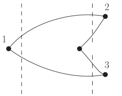
In the formalism one considers initial and final meson creation operators I, II, given above (see in Appendix B the Table 6 of lowest operators and their forms), and composes the decay matrix element as shown in Figure 1 where vertices are operators entering in the bilinears , and lines denote quark Green’s functions , etc. so that matrix element corresponding to Figure 1 is
| (5) |
As was shown in Badalian et al. (2007); Simonov (2008) in the approximation where one neglects influence of spin forces on wave functions, one can replace
| (6) |
where is quadratic Green’s function, are projection operators, the variables are the averaged kinetic energies and are the pole masses.
Our physical matrix element corresponding to the decay can be obtained from (5) by projecting the chosen intermediate states, as shown by dashed lines in Figure 1.
As a result as shown in Simonov (2008); Simonov and Veselov (2009a) the physical projected matrix element has the form
| (7) |
where is the number of colours, and . The expressions for , are proportional to Dirac traces of the projector operators and are given in [13,14]. We point that the w.f in (7) are no longer full w.f. of mesons, but the radial part divided by , while the angular part of the w.f. is accounted for in the factor . Important role is played by average values of quark kinetic energies, inside heavy-light mesons in their c.m. systems (if one neglects c.m. motion of these mesons). The numbers of are computed from the relativistic string Hamiltonian in Badalian and Danilkin (2009); *Badalian:2004gw; *Badalian:2008dv; *Badalian:2007zz; Badalian et al. (2009b); *Badalian:2009bu; *Badalian:2004xv. In practical calculations it is more useful to exploit the reduction of the bispinor wave functions in (4), as and , see details in Appendix B. The resulting matrix element has the same form as in (7) but with , where is given in Table 7 and is proportional (see Appendix C).
Now one can define the selfenergy part in sector I due to sector II in the intermediate state, which is
| (8) |
and the total Green’s function in sector I can be written as (sum over bound states only)
| (9) |
where ellipsis implies terms of higher order in and this can be summed up as
| (10) |
where matrix .
Note, that in (10) the Green’s function is actually a projection of the coupled-channel system on the original unperturbed wave functions . In reality wave functions of the coupled-channel system differ from the latter and acquire continuous spectrum pieces above the decay threshold, and hence need a special treatment to be discussed below.
The new spectrum is obtained from (10) as
| (11) |
for one level in sector I it simplifies
| (12) |
which yields energy shift and width in the first order approximation in :
| (13) |
In the next order one should solve the transcendental in one-channel equation (12), which is valid when is large, but .
Below the decay threshold one can diagonalize the matrix in (10) with unitary matrices
| (14) |
and the Green’s function acquires the form
| (15) |
In this way become new orthogonal states comprising all effects of mixture between bound states due to closed channels. The same procedure can be applied for open channels (above the decay threshold) when one neglects the widths of the levels, i.e. imaginary part of .
One can define interaction in sector I due to sector II,
| (16) |
with
| (17) |
| (18) |
or, in momentum space
| (19) |
where Now the one-channel Hamiltonian in sector I is augmented by the term ,
| (20) |
Note, that the coupled-channel (CC) interaction can be strong enough to support its own bound states, as was studied in Badalian et al. (1982), where this type of resonances was called the CC resonances.
Let us now turn to the relativistic string Hamiltonian (RSH) , derived from the gauge-invariant meson Green’s function in QCD in the one-channel case in Dubin et al. (1993); *Badalian:2008sv. This Hamiltonian has been successfully applied to light mesons Badalian and Bakker (2002), heavy-light mesons Badalian et al. (2007); Kalashnikova et al. (2001); *Badalian:2007yr; *Badalian:2009cx, and heavy quarkonia Badalian and Danilkin (2009); *Badalian:2004gw; *Badalian:2008dv; *Badalian:2007zz; Badalian et al. (2009b); *Badalian:2009bu; *Badalian:2004xv and has a simple form:
| (21) |
| (22) |
In general, the quantity appearing in this expression is an operator, which in the so-called einbein approximation is defined by an extremum condition . A simple expression for the spin-averaged mass follows from the RSH (21)
| (23) |
Here, the excitation energy depends on the reduced mass . The formula (23) does not contain any additive constant; for a light quark (e.g. in the -meson) a negative (not small) nonperturbative self-energy term appears, proportional to ; it has to be added to their masses Simonov (2001); *DiGiacomo:2004ff. In the case of charmonium this term is small; the variables , the excitation energy , and the w.f. are calculated from the Hamiltonian (21) and two extremum conditions , Dubin et al. (1993); *Badalian:2008sv; Simonov (1999):
| (24) |
The potential in (22) is derived in the framework of the Field Correlator Method Dosch (1987); *Dosch:1988ha; *Simonov:1987rn; Di Giacomo et al. (2002); Badalian and Danilkin (2009); *Badalian:2004gw; *Badalian:2008dv; *Badalian:2007zz and is the sum of a pure scalar confining term and a gluon-exchange part,
| (25) |
where the vector coupling is taken in the two-loop approximation and possesses two important features: the asymptotic freedom behavior at small distances, defined by the QCD constant [which is considered to be known, because is directly expressed via the QCD constant in the renormalization scheme]; it freezes at large distances. Details about the effective fine-structure constant can be found in Ref. Badalian and Danilkin (2009); *Badalian:2004gw; *Badalian:2008dv; *Badalian:2007zz.
III RESONANCES IN THE DECAY SECTOR
As it was discussed in Badalian et al. (1982), the situation of two coupled sectors I, II, and , can be treated in two ways:
1) as a coupled system of matrix Green’s functions,
2) as a reduction of two-sector problem to the one-sector problem with energy-dependent “potential” or 333Note, that a parallel treatment of the open channel problem in nuclear reactions is developed by H.Feshbach with the help of the projection operators in his unified theory of nuclear reactions Feshbach (1962).. We shall continue our one-channel treatment from the point of view of Sector II. In the same way as it was done before, one can define the “potential”
| (26) |
Defining also one can write
| (27) |
and as a result one obtains a system of equations in sector II
| (28) |
where is a direct interaction between two color singlet mesons, which we neglect in the first approximation, is the same as in (21) but for equal to masses of mesons with quantum numbers . Neglecting , one can easily rewrite (28) for the separable interaction (27)
| (29) |
where
| (30) |
Introducing , and integrating both sides of (29) with , one has from (29)
| (31) |
with the same as in (8), and the equation for eigenvalues is again (11).
Since the CC interaction (27) is separable, one can study the structure of the spectrum of our CC problem in more detail; in particular, whether there can appear poles (CC resonances in terminology of Badalian et al. (1982)) due to strong CC interaction, which are additional to the one-sector spectrum of poles , the latter being simply shifted by CC. As was argued in Badalian et al. (1982), we define the integral
| (32) |
According to Badalian et al. (1982), a bound state in a single channel due to CC with the sector I can exist, if in the region, where (32) is real (below threshold ), it becomes larger than one
| (33) |
In the momentum space one has
| (34) |
which yields the same equation as in (31). As before in Eq. (11), one obtains from (34) the equation , which defines all poles in the cut plane below thresholds and on the second, and higher Riemann sheets.
IV THEORY OF COUPLED-CHANNEL RESONANCES BASED ON THE WEINBERG EIGENVALUE METHOD
The coupled-channel problem can be quantified using the eigenvalue analysis introduced by Weinberg Weinberg (1963); *newton:319; *Smithies1958. Although this formalism has been developed long ago, it is still not widely known. That is why in this section we present a short summary of corresponding formulae leaving details to the Appendix D.
The Schrodinger equation for two-body like Hamiltonian can be written in the standard (time-independent) way
| (35) |
where E is a spectral variable, is an energy eigenstate and is an operator, which in the nonlocal case acts in (35) as . In the Weinberg method, instead, w.f. are the eigensolutions of
| (36) |
where E is the continuous parameter entering w.f. and the index labels the discrete eigenvalues and eigenvectors. The Weinberg eigenvalue is the potential scale and thus the spectrum consists of all the potential rescalings that give solution to that equation, for given energy .
Let us now turn to the question of the rigorous definition of the resonance wave function and start with the one-state situation, when only one state is considered in sector II, with fixed . The induced interaction has the form (27) and direct interaction is neglected for simplicity. One can exploit the WEM Weinberg (1963); *newton:319; *Smithies1958, and divide the potential in (32) by an energy-dependent factor considering instead of Eq. (28) another one (with
| (37) |
which defines for each the eigenvalue and eigenfunction , with the boundary conditions
| (38) |
For one has instead In the WEM, resonance structures as well as bound sates can be obtained in terms of Weinberg eigenvalues . Note, that a solution of integro-differential equation (37) in the coordinate space can satisfy these boundary conditions for each energy only for some discrete value of . Compare e.g. with the case of bound states (energy below threshold), where boundary conditions at origin and infinity can be matched only for discrete energy in standard formalism ( or at some for any in WEM, with the relation .
The normalization of wave functions is
| (39) |
Note, that is real analytic (holomorphic) for all except for pole positions, and the off-shell -matrix looks as (see Weinberg (1963); *newton:319; *Smithies1958 and Appendix D for a derivation)
| (40) |
with
| (41) |
| (42) |
and the Green’s function (10) has the form
The sum over is fast converging as one can see from the example of square well and other potentials fast decreasing at Narodetsky (1981); *Narodetsky:1969jf; *Herzenberg; *Fuda. Therefore in what follows in our calculations we shall consider only one term in the sum over , which is relevant for a given threshold.
The Breit-Wigner resonances in sector II are obtained from the condition that for some , , and
| (43) |
Note, that the corresponding serves as the normalized resonance wave function and can be used e.g. to calculate average values of some operator or perturbative shift of resonance position. The Green’s function with account of channel coupling can be written near the pole (resonance) as
| (44) |
As it is seen from (37), the introduction of WEM eigenvalue in equations reduces to the replacement , hence the resulting equation for the calculation of is
| (45) |
Eq.(45) is of the -th power in , when levels are taken into account, and this yields roots , . Total number of poles is given by solutions , , where depends on behavior of .
We started formally with the one channel in sector II, i.e. with fixed , hence in in Eq.(45) the sum over (cf. Eq.(8)) reduces to one term. However, for several states one has equation (28) with interaction kernel as a matrix in indices , and if in (37) does not depend on , then as a result one has for the same Eq.(45), but now with , which corresponds fully to (8), i.e. contains the sum over .
Let us discuss how the basic equation (45) changes for many channels . We start with Eq. (29), which is equivalent to (37), when one introduces in (29) in the denominator on the r.h.s. the factor . Multiplying both sides of this modified Eq. (29) with and integrating and summing over one obtains equation similar to (31)
| (46) |
where , and is the same, as in (8), i.e. again with the sum over . The resulting equation to determine is again (45), and all equations (37)-(39) have the same form, if one takes into account, that is a column of components and is a matrix in indices .
Finally, the separate components are found through via (cf. (29))
| (47) |
and partial widths of the resonance are found in lowest approximation as (for one channel in sector I)
| (48) |
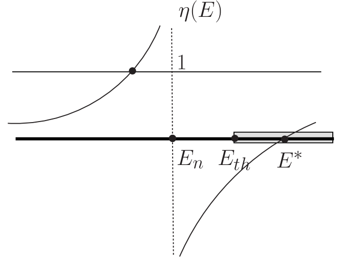
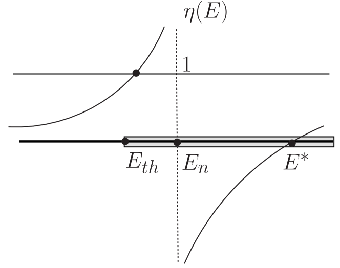
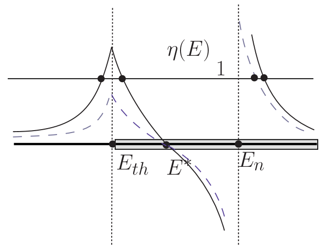
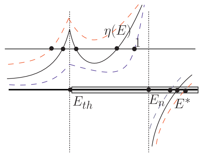
To understand the possible origin and position of resonances in our CC problems, one can consider several typical cases, depending on relative positions of bare resonances and thresholds . Consider first one state in sector I, one state in sector II, then for , and changes sign at . The resulting qualitative picture of is shown in Figure 2 for three cases: (Fig. 2(a)); (Fig. 2(b,d)); (Fig.2(c)). In Fig.2(a,b) one can see one critical energy for which . This point corresponds to the shifted energy level .
Note the possibility of a pair of additional roots of equation , when , and
| (49) |
The condition (49) defines the strength of CC interaction in the situation depicted in Fig.2(c,d) which is necessary one additional pole near the threshold energy (see Appendix E for details). As we shall show below in section VI, the situation of Fig.2(d) is most likely realized in the state of charmonium, where the threshold peak corresponds to the state. In this case actually two close-by thresholds are present ( and ), and as will be seen, the experimentally observed situation with one peak at lowest threshold and wide structure near GeV indeed occurs.
(a) case
(b) case
(c) case
(d) case
Consider now the case of two levels in sector I, and ; and one (or more) state in sector II. The equation for has the form
| (50) |
with , and the result
| (51) |
where for notational convenience we have suppressed the energy dependence of the .
Near can be identified with the one-channel eigenvalues and , namely for and one has
| (52) |
The situation with trajectories is in general rather complicated, and we describe below only one case when where , and in case of strong mixing of channels 1 and 2 the point , where lies between and . (The position of is irrelevant for the situation where all imaginary parts are neglected). However for weak mixing of channels 1, 2 roots never coincide. One can see from (51) that in the weak mixing case only two poles remain, corresponding to shifted levels and no new resonances appear at least for .
V MIXING OF STATES IN THE WEINBERG FORMALISM
The WEM solves the important problem of constructing the full set of orthogonal states in the coupled channel problem, and thus the problem of mixing of states. This is nontrivial in the situation under investigation, since the interaction in the sector I induced by the coupling to the sector II, , Eq. (16), is energy dependent and hence violates the orthogonality of eigenstates. In addition, for energies above threshold, this interaction is complex and makes the corresponding states the resonances, which cannot be normalized and orthogonalized to each other in the ordinary way. Happily, WEM allows to define all states and their mixing in the mathematically rigorous way, as we shall now show.
We start with the formulation in sector I and write starting from (20) the WEM equation
| (54) |
while the unperturbed states satisfy
| (55) |
Note, that depend on energy , while do not. Similarly to (39), the orthogonality condition is
| (56) |
Consider now the expansion of a WEM state in the set of states,
| (57) |
Taking into account, that
| (58) |
and multiplaying both sides of (54) with and integrating over , one obtains
| (59) |
Thus one obtains the equation for eigenvalues
| (60) |
which coincides with (45), obtained in sector II. Now we are specifically interested in the coefficients , for two different eigenvalues .
The first condition follows from (56), (59)
| (61) |
It is convenient to introduce reduced coefficients:
| (62) |
Then the solution for two eigenvalues in (60) is
| (63) |
here and further for notational convenience we will suppress the energy dependence of the . The normalization condition has the form
| (64) |
Let us take one concrete example of two states in the subthreshold region (e.g. ( and ( states of charmonium, however at this stage they are not specified).
Keeping only two states e.g. for and , one can write for ,
| (65) |
Note, that the appearance of coefficients is not accidental since is symmetric in .
We are thus e.g. looking for the shifted and mixed state, denoted by , and the same for state, denoted by .
| (66) |
To find , one can use the second equation in (64), which yields
| (67) |
This gives the condition , which is identically satisfied, and the final result for
| (68) |
Note, that the sign of is connected with the corresponding choice of the root in (63), for (lower in energy state) we have chosen the sign .
It is clear, that depends on and therefore to define finally the mixing coefficient, one should fix the energy. E.g. for the state , the eigenvalue crosses the line at the resonance position , complex in general, and the mixing coefficient of interest from (65) is , while the mixing coefficient of the state is to be taken at , .
Hence, for small shifts , and energy independent , one recovers the symmetry condition
| (69) |
Finally, one should connect normalizations of and . This can be done, if one considers the limiting case of one channel , where according to (58), (56), one has
| (70) |
and for (at the resonance position), , and for one level from (60) one has . Hence in the one-channel – one-level limit we have
| (71) |
Therefore if only one level n is kept, then the normalized WEM states can be defined as
| (72) |
and finally the standard normalized mixing coefficients are
| (73) |
where . One can see, that in general coefficients are less than unity due to ratios of square roots. We finally write for
| (74) |
Another (and physically more motivated) normalization for follows from (44), which can be written as
Estimating , , one obtains , and the defacto wave functions is , which is close to (72) for .
VI RESULTS AND DISCUSSION
The formalism given in this paper is based on the explicit knowledge of wave functions in both sectors I and II and yields the CC interaction operator expressed via the overlap integrals, see Eq.(8). The resulting effective interaction in each sector is energy dependent due to , and violates usual orthonormality properties for wave functions. Moreover, new states appear for energies above thresholds, and one needs a rigorous formalism to treat the complete set of eigenfunctions for such operators. The WEM is indispensable for this purpose. In Eq.(45) explicit conditions are written down for Weinberg eigenvalues . It is important, that has simple analytic properties in the -plane. Therefore physical quantities expressed via , like scattering amplitude (E.1) or production cross-section (E.2) have a definite analytic expression near the pole(s), different from the Breit-Wigner form in general. This property is more important in case of the complicated arrangement of thresholds and poles, as it is in the case of , see below.
Another practical advantage of WEM is the complete set of states for each energy , allowing to define unambiguously symmetric mixing coefficients, as it was explained in section V.
Before a detailed discussion of results, one should stress two main features of the closed channel pole behavior under the influence of CC: 1) CC is attractive for all states below CC threshold; 2) CC is attractive in some region above threshold and repulsive for (in the limit of small width). Both statements follow from the condition or in (8). As will be seen in the simplest case of one channel with lowest threshold, the pole occurs in the attractive zone of the channel and hence moves down with increasing coupling.
| State (Thresholds) | Theory | Experiment |
|---|---|---|
| 3.068 | 3.068 | |
| 3.488 | 3.525 | |
| 3.678 | 3.674 | |
| 3.729 | ||
| 3.787 | 3.771 | |
| 3.872 | ||
| 3.954 | 3.930 | |
| 4.014 | ||
| 4.116 | 4.040 |
Below we give several examples of WEM application to different problems in CC dynamics. We shall consider
i) How CC interaction changes states as compared to one-channel calculations. We will calculate energy shifts and widths for state and also mixing between and states.
ii) We calculate eigenvalues and amplitudes in the state in connection with the bare level and resulting resonance.
To illustrate this formalism we will consider situation with one level in sector I and one (or many) level(s) in sector II. In Table 1 we present charmonium mass spectrum in the single-channel approach (SCA) derived from RSH (21) (see for example Badalian and Danilkin (2009); *Badalian:2004gw; *Badalian:2008dv; *Badalian:2007zz) in comparison with experimental data and showing the thresholds.
VI.1 levels
As a first numerical example we consider the mass shifts and widths of the states. For these levels the corresponding factors are ; ; (see Appendix B,C) and the transition matrix element is rewritten in the following form (see appendix C and equation (C.2))
| (75) |
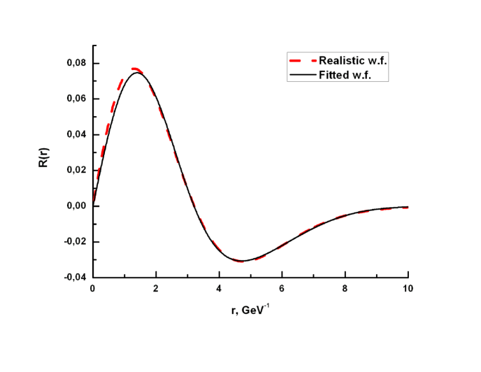
where is channel coupling parameter which is proportional (see Appendix C) and , where the averaged kinetic energies of heavy and light quarks in D meson GeV, GeV are taken from Badalian et al. (2007). In Eq.(75) are series of oscillator functions, which are fitted to realistic w.f. (see Appendix A). We obtain the latter from the solution of RSH (21) Badalian and Danilkin (2009); *Badalian:2004gw; *Badalian:2008dv; *Badalian:2007zz.
The widths and mass shifts are obtained from averaging over initial (i) and summing over final (k,j) polarizations. Note that the final formulas for the width in channels , and differ by spin factors, which yield the ratio 1:4:7. From Eq.(13, 48) one can write the width taking into account relativistic corrections
| (76) |
where are the masses of the corresponding mesons.
| Channel | p, GeV | , MeV |
|---|---|---|
| 0.777 | 0.31 | |
| 0.576 | 25.5 | |
| 0.227 | 17.8 |
| Ratio | Experiment Aubert et al. (2009) | This paper | Barnes et al. (2005); *Barnes:1991em |
|---|---|---|---|
| 0.012 | 0.003 | ||
| 0.70 | 1.0 |
| State | Total | |||
|---|---|---|---|---|
| -5 | -19 | -30 | -54 | |
| -15 | -41 | -56 | -112 | |
| -6 | -10 | -45 | -61 |
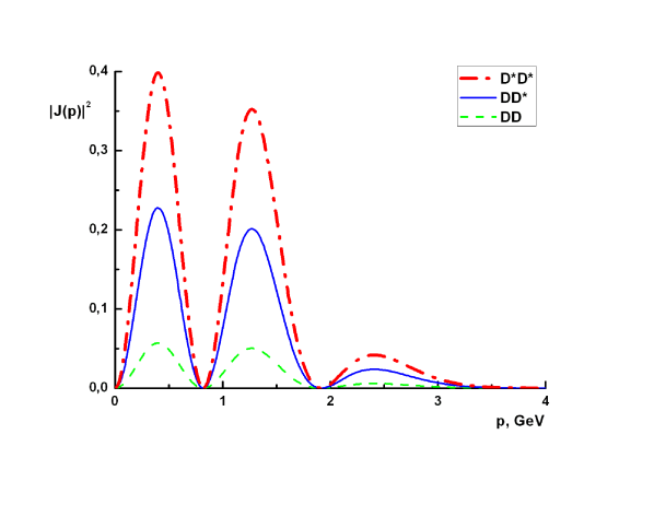
It is important that the value of the decay width strongly depends on transition matrix element. This is illustrated by the behavior of for state. As it can be seen from Figure 4, is oscillating and has two zeros, corresponding to the wave function nodes. In the small width approximation (13) the width and shift of level will vanish when approaches zero on Figure 4. It is not a physical situation, and in the next approximation one should solve Eq.(3) in complex plane and take into account possible mixing between states due to open channels. For instance it can be 3S-2S, or 3S-2D mixing. Due to the mixing, the w.f. of the ”pure” states changes and minima in Figure 4 can be filled in by admixed states. In Tables 2, 3 are given the small width values for state of charmonium in the channel, illustrating the zeros discussed above.
In WEM the shifted level positions are defined from Eq. (45) and for one obtains the picture shown in Figure 4. The level shifts calculated from Eq.(13) are given in Table 4. One can note relatively small shifts ( MeV) as compared to Kalashnikova (2005); *Baru:2003qq; Barnes and Swanson (2008), where and SHO model was used, whereas in our case more complicated realistic wave functions were exploited.
In addition we have considered mixing between and levels via threshold, which turned out to be small, with the mixing angle (defined as in (74)) .
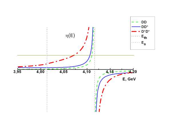
VI.2 -level
A separate discussion is needed for the s-wave decay to charmed mesons. We take as an explicit example the decay . Note, that due to positive C parity the s-wave strength is mostly concentrated in the channel. In this case, the situation of Figure 2(c,d) is realized when can cross the unity line at several energy values, thus producing several resonances. In our calculations we show in Figure 5 which correspond to different values of channel coupling parameter in the region around the standard value ( GeV). As it can be seen, intercepts the line three times. However we have to take into account imaginary parts above the thresholds. The simplest way is to calculate factor which appears in the squared t-matrix (40). The result is the two-resonance structure, one of which is near threshold GeV and another one near GeV, the latter becomes increasingly broad with increasing coupling to open channel. In the recent work Kalashnikova and Nefediev (2009) a similar form of the first peak was suggested.
(a) One threshold, =3.872 GeV.
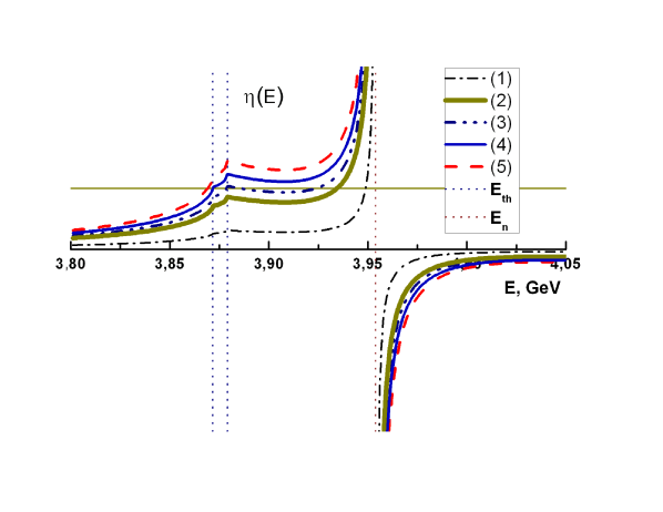
(b) Two thresholds, =3.872; 3.879 GeV.
We note, that the factor is relevant for the t-matrix of scattering, while new charmonium resonances were observed in production cross sections like or . Therefore we define the production yield given in (E.2) and show in Figure 6 the quantity . In our approximation ( and thresholds coincide and there is no connection to and channels) one can see the double peak structure for ; the first peak at GeV is accompanied by a wide peak around 3.940 GeV.
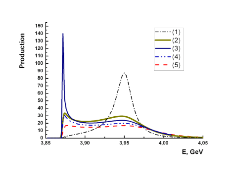
However, with increasing , when , the peak in Fig. 6 at 3940 becomes flat, while the lower peak at 3.872 GeV is narrow and high. This picture corresponds to the experimental situation.
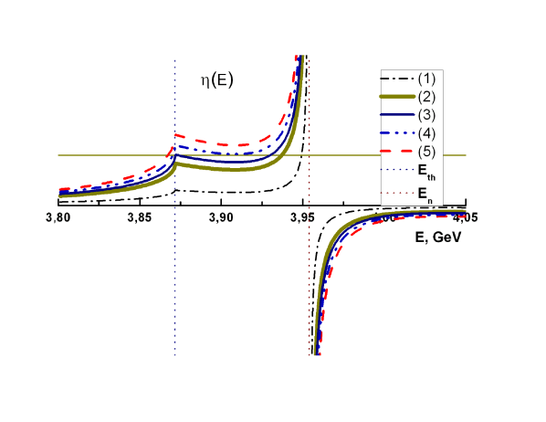
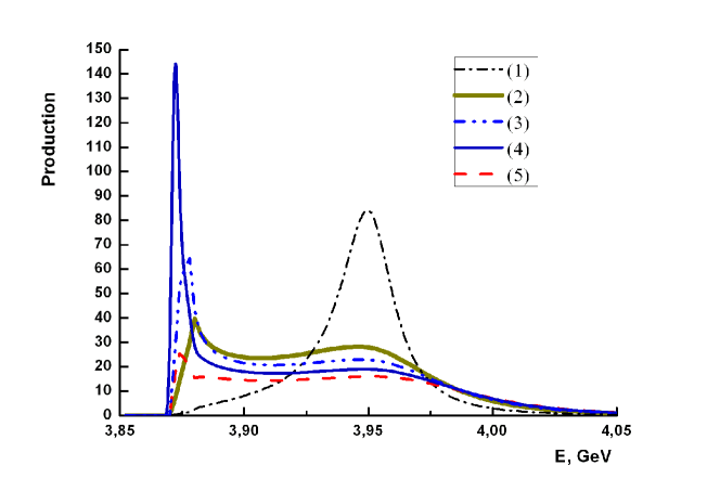
The case when both thresholds and are taken into account, is illustrated by Figure 5 for and Figure 7 for the production cross section. As can be seen, the curves for production cross section depend strongly on channel coupling parameter . For (line (2)) which is 30% smaller than the nominal value GeV) one can see a peak at the higher threshold and a wider peak at GeV, however for (line (4)), the GeV peak flattens and simultaneously(!), the peak appears at the lower threshold , while only a week cusp is seen at the higher threshold . Surprisingly, the isotopically equivalent thresholds (which we take into account with equal weight) due to different position in energy plane, provide finally the asymmetric picture observed in experiment Abe et al. (2007); *Pakhlova:2008di; *Yuan:2009iu.
VII SUMMARY
We have formulated equations for Green’s functions of strongly coupled sectors, where new resonances can appear due to CC interaction. We found that the best formalism for the CC induced energy-dependent interaction is the Weinberg eigenvalue method. Conditions for the poles and their positions were systematically studied in case of -wave and -wave channel coupling. In the first case one finds only displacement of poles, while in the second new resonances appear, and in the case two peaks at 3.872 and 3.940 GeV were found with the height depending on the coupling constant . Moreover, we have shown in Fig.7, that at one value of the lower peak is at the threshold (but not at the threshold) and at the same time the upper peak at 3.940 GeV flattens. This situation corresponds to the experimental data Abe et al. (2007); *Pakhlova:2008di; *Yuan:2009iu and supports our dynamical CC mechanism.
Mixing of states was formulated in WEM and found to be small, while shifts of are of the order 50-80 MeV, which signals necessity of mass renormalization.
The method developed in the present paper, provides a rigorous definition of resonance wave functions and mixings in the case of strongly coupled channels.
ACKNOWLEDGMENTS
The authors are grateful to Yu.S.Kalashnikova for numerous discussions, suggestions and help, to A.M.Badalian for useful discussions and remarks, to A.I.Veselov for suggestions and help with computer programs, and to A.E.Kudryavtsev for good questions.
The financial help of Dynasty Foundation to I.V.D. and RFFI grant 09-02-00629a and grant NS-4961.2008.2 is gratefully acknowledged.
References
- Eichten et al. (1980) E. Eichten, K. Gottfried, T. Kinoshita, K. D. Lane, and T.-M. Yan, Phys. Rev. D21, 203 (1980)
- Eichten et al. (1978) E. Eichten, K. Gottfried, T. Kinoshita, K. D. Lane, and T.-M. Yan, Phys. Rev. D17, 3090 (1978)
- Eichten et al. (1976) E. Eichten, K. Gottfried, T. Kinoshita, K. D. Lane, and T.-M. Yan, Phys. Rev. Lett. 36, 500 (1976)
- Geiger and Isgur (1993) P. Geiger and N. Isgur, Phys. Rev. D47, 5050 (1993)
- Geiger and Isgur (1991a) P. Geiger and N. Isgur, Phys. Rev. Lett. 67, 1066 (1991a)
- Geiger and Isgur (1991b) P. Geiger and N. Isgur, Phys. Rev. D44, 799 (1991b)
- Geiger and Isgur (1990) P. Geiger and N. Isgur, Phys. Rev. D41, 1595 (1990)
- van Beveren et al. (1983) E. van Beveren, G. Rupp, T. A. Rijken, and C. Dullemond, Phys. Rev. D27, 1527 (1983)
- van Beveren et al. (1980) E. van Beveren, C. Dullemond, and G. Rupp, Phys. Rev. D21, 772 (1980)
- Tornqvist (1995) N. A. Tornqvist, Z. Phys. C68, 647 (1995), eprint hep-ph/9504372
- Tornqvist and Roos (1996) N. A. Tornqvist and M. Roos, Phys. Rev. Lett. 76, 1575 (1996), eprint hep-ph/9511210
- Badalian et al. (1982) A. M. Badalian, L. P. Kok, M. I. Polikarpov, and Y. A. Simonov, Phys. Rept. 82, 31 (1982)
- Kalashnikova (2005) Y. S. Kalashnikova, Phys. Rev. D72, 034010 (2005), eprint hep-ph/0506270
- Baru et al. (2004) V. Baru, J. Haidenbauer, C. Hanhart, Y. Kalashnikova, and A. E. Kudryavtsev, Phys. Lett. B586, 53 (2004), eprint hep-ph/0308129
- Barnes and Swanson (2008) T. Barnes and E. S. Swanson, Phys. Rev. C77, 055206 (2008), eprint 0711.2080
- Pennington and Wilson (2007) M. R. Pennington and D. J. Wilson, Phys. Rev. D76, 077502 (2007), eprint 0704.3384
- Dubin et al. (1993) A. Y. Dubin, A. B. Kaidalov, and Y. A. Simonov, Phys. Atom. Nucl. 56, 1745 (1993), eprint hep-ph/9311344
- Badalian et al. (2008a) A. M. Badalian, A. V. Nefediev, and Y. A. Simonov, Phys. Rev. D78, 114020 (2008a), eprint 0811.2599
- Dosch (1987) H. G. Dosch, Phys. Lett. B190, 177 (1987)
- Dosch and Simonov (1988) H. G. Dosch and Y. A. Simonov, Phys. Lett. B205, 339 (1988)
- Simonov (1988) Y. A. Simonov, Nucl. Phys. B307, 512 (1988)
- Di Giacomo et al. (2002) A. Di Giacomo, H. G. Dosch, V. I. Shevchenko, and Y. A. Simonov, Phys. Rept. 372, 319 (2002), eprint hep-ph/0007223
- Badalian and Danilkin (2009) A. M. Badalian and I. V. Danilkin, Phys. Atom. Nucl. 72, 1206 (2009), eprint 0801.1614
- Badalian et al. (2005) A. M. Badalian, A. I. Veselov, and B. L. G. Bakker, J. Phys. G31, 417 (2005), eprint hep-ph/0411291
- Badalian et al. (2009a) A. M. Badalian, B. L. G. Bakker, and I. V. Danilkin, Phys. Atom. Nucl. 72, 638 (2009a), eprint 0805.2291
- Badalian and Bakker (2007) A. M. Badalian and B. L. G. Bakker, Phys. Atom. Nucl. 70, 1764 (2007)
- Simonov (2008) Y. A. Simonov, Phys. Atom. Nucl. 71, 1048 (2008), eprint 0711.3626
- Simonov and Veselov (2009a) Y. A. Simonov and A. I. Veselov, Phys. Rev. D79, 034024 (2009a), eprint 0804.4635
- Simonov and Veselov (2009b) Y. A. Simonov and A. I. Veselov, Phys. Lett. B671, 55 (2009b), eprint 0805.4499
- Simonov and Veselov (2008) Y. A. Simonov and A. I. Veselov, JETP Lett. 88, 5 (2008), eprint 0805.4518
- Barnes et al. (2005) T. Barnes, S. Godfrey, and E. S. Swanson, Phys. Rev. D72, 054026 (2005), eprint hep-ph/0505002
- Barnes and Swanson (1992) T. Barnes and E. S. Swanson, Phys. Rev. D46, 131 (1992)
- Ackleh et al. (1996) E. S. Ackleh, T. Barnes, and E. S. Swanson, Phys. Rev. D54, 6811 (1996), eprint hep-ph/9604355
- Micu (1969) L. Micu, Nucl. Phys. B10, 521 (1969)
- Le Yaouanc et al. (1973) A. Le Yaouanc, L. Oliver, O. Pene, and J. C. Raynal, Phys. Rev. D8, 2223 (1973)
- Le Yaouanc et al. (1977a) A. Le Yaouanc, L. Oliver, O. Pene, and J. C. Raynal, Phys. Lett. B71, 397 (1977a)
- Le Yaouanc et al. (1977b) A. Le Yaouanc, L. Oliver, O. Pene, and J. C. Raynal, Phys. Lett. B72, 57 (1977b)
- Weinberg (1963) S. Weinberg, Phys. Rev. 131, 440 (1963)
- Newton (1960) R. G. Newton, Journal of Mathematical Physics 1, 319 (1960)
- Smithies (1958) F. Smithies, Integral Equation (Cambridge University Press, New York, 1958)
- Narodetsky (1981) I. M. Narodetsky, Riv. Nuovo Cim. 4N7, 1 (1981)
- Narodetsky (1969) I. M. Narodetsky, Yad. Fiz. 9, 1086 (1969)
- Herzenberg and Mandl (1963) A. Herzenberg and F. Mandl, Physics Letters 6, 288 (1963), ISSN 0031-9163
- Fuda (1968) M. G. Fuda, Phys. Rev. 174, 1134 (1968)
- Abe et al. (2007) K. Abe et al., Phys. Rev. Lett. 98, 082001 (2007), eprint hep-ex/0507019
- Pakhlova (2008) G. V. Pakhlova (2008), eprint 0810.4114
- Yuan (2009) C.-Z. Yuan (Belle) (2009), eprint 0910.3138
- Badalian et al. (2007) A. M. Badalian, B. L. G. Bakker, and Y. A. Simonov, Phys. Rev. D75, 116001 (2007), eprint hep-ph/0702157
- Hashimoto et al. (1999) S. Hashimoto et al., Phys. Rev. D61, 014502 (1999), eprint hep-ph/9906376
- Becirevic et al. (2005) D. Becirevic et al., Nucl. Phys. B705, 339 (2005), eprint hep-ph/0403217
- Brommel et al. (2007) D. Brommel et al. (The QCDSF), PoS LAT2007, 364 (2007), eprint 0710.2100
- Bowler et al. (1996) K. C. Bowler et al. (UKQCD), Phys. Rev. D54, 3619 (1996), eprint hep-lat/9601022
- Badalian et al. (2009b) A. M. Badalian, B. L. G. Bakker, and I. V. Danilkin, Phys. Rev. D79, 037505 (2009b), eprint 0812.2136
- Badalian et al. (2009c) A. M. Badalian, B. L. G. Bakker, and I. V. Danilkin (2009c), eprint 0903.3643
- Badalian et al. (2004) A. M. Badalian, A. I. Veselov, and B. L. G. Bakker, Phys. Rev. D70, 016007 (2004)
- Badalian and Bakker (2002) A. M. Badalian and B. L. G. Bakker, Phys. Rev. D66, 034025 (2002), eprint hep-ph/0202246
- Kalashnikova et al. (2001) Y. S. Kalashnikova, A. V. Nefediev, and Y. A. Simonov, Phys. Rev. D64, 014037 (2001), eprint hep-ph/0103274
- Badalian et al. (2008b) A. M. Badalian, Y. A. Simonov, and M. A. Trusov, Phys. Rev. D77, 074017 (2008b), eprint 0712.3943
- Badalian et al. (2009d) A. M. Badalian, B. L. G. Bakker, and I. V. Danilkin (2009d), eprint 0911.4634
- Simonov (2001) Y. A. Simonov, Phys. Lett. B515, 137 (2001), eprint hep-ph/0105141
- Di Giacomo and Simonov (2004) A. Di Giacomo and Y. A. Simonov, Phys. Lett. B595, 368 (2004), eprint hep-ph/0404044
- Simonov (1999) Y. A. Simonov, in Lectures given at 17th Autumn School: QCD: Perturbative or Nonperturbative? (Lisbon, 1999), eprint hep-ph/9911237
- Feshbach (1962) H. Feshbach, Ann. Phys. 19, 287 (1962)
- Yao et al. (2006) W. M. Yao et al. (Particle Data Group), J. Phys. G33, 1 (2006)
- Aubert et al. (2009) B. Aubert et al. (BABAR), Phys. Rev. D79, 092001 (2009), eprint 0903.1597
- Kalashnikova and Nefediev (2009) Y. S. Kalashnikova and A. V. Nefediev, Phys. Rev. D80, 074004 (2009), eprint 0907.4901
Appendix A
WAVE FUNCTIONS
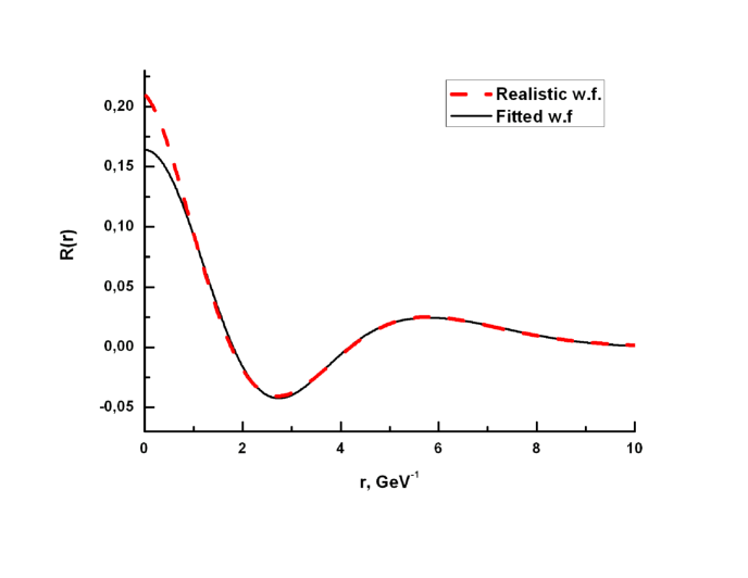
In Eq.(75) , and are series of oscillator wave functions, which are fitted to realistic wave functions. We obtain them from the solution of the Relativistic String Hamiltonian (21), described in Dubin et al. (1993); *Badalian:2008sv; Badalian and Danilkin (2009); *Badalian:2004gw; *Badalian:2008dv; *Badalian:2007zz; Badalian et al. (2009b); *Badalian:2009bu; *Badalian:2004xv.
In position space the basic SHO radial wave function is given by
| (A.1) | |||
where is the SHO wave function parameter, and is an associated Laguerre polynomial. The realistic radial wave function can be represented as an expansion in the full set of oscillator radial functions:
| State | Coefficients | |||||
|---|---|---|---|---|---|---|
| Charmonium | ||||||
| 0.70 | ||||||
| 0.53 | ||||||
| 0.46 | ||||||
| 0.48 | ||||||
| D meson | ||||||
| 1S | 0.48 | c=1 | ||||
(a)
(b)
Appendix B
THE VERTEX OPERATORS AND SPINOR EXPRESSIONS IN THE FORM
Our purpose here is to go from Eq.(8), where is the trace of form to the or spinor form, defining in this way
We consider operators of the form , with consisting of Dirac matrices and derivatives . To proceed to the form, one exploits the limit of the heavy quark mass, so that for the light quark in the heavy-light meson the Dirac equation can be used, and one can use symbolically Dirac one-body equation, , so that for , one has . One can also use connection , where , so that .
| form. | |||
|---|---|---|---|
| 1 | |||
Note, that spin indices of charge-conjugated spinors are connected to ordinary spinors by matrix : , and for one has:
| (B.1) |
where the notation implies, that operator acts on the left. We are considering 7 lowest states and display in the Table 6 the operator , the corresponding quantum numbers , spectroscopic notation and the equivalent form for the same vertex in the last column. We are using in the Table 6 the following notations
Note, that in the form one has:
| - | |||||
| - | |||||
| - | |||||
| - | - | ||||
| - | - | ||||
In the form one can write wave function of charmonium and D-mesons ) as and normalize it as
| (B.2) |
Defining , the normalization condition for angular part takes the form . Then can be written as in (7), but can be found in spinor form as
| (B.3) |
see Table 7, and all are normalized as written above. Hence e.g.
Appendix C
THE PAIR-CREATION VERTEX
In the same way we consider here the reduction of the pair-creation vertex, taking for light quarks as solutions of Dirac equation and writing the effective string-breaking Lagrangian as
| (C.1) |
and we have denoted: ; is the Dirac eigenvalue , is the spinor of antiquark, is the same as in Eq. (3).
One can take in (C.1) the averaged value of the denominator which effectively redefines our vertex constant . As a result the reduced form of the matrix element in Eq. (8) assumes the form
| (C.2) |
where is given in Table 7 and . One can find values of , , in Table 8, and persuade oneself, that is rather stable for different and numerically
To check consistency of our approximation of putting average values into denominator, we have compared normlization conditions of bispinors , and found that the term with denominator contributes around 20%, and we expect the same accuracy in definition of . Actually, we are always varying in the region around the nominal value .
One can also check at this point how the vertex goes over into the reduced form . E.g. for the state decaying into one has in the heavy quark mass limit (see e.g. [13,14]). , and GeV is the average energy of the light quark, which coincides with 1/2 of the denominator in , while from Table 7 is . Thus indeed one has equality .
For practical reasons we have used for our calculations the reduced forms everywhere.
| 0 | 0.3 | 0.39 | |
|---|---|---|---|
| 0.65 | 0.493 | 0.424 | |
| 0.80 | 0.584 | 0.509 | |
| 0.838 | 0.617 | 0.539 | |
| 0.573 | 0.486 | 0.463 | |
| 0 | -0.198 | -0.273 |
In the nonrelativistic limit one has
| (C.3) |
and for the plane-wave (free) quarks, , one has
| (C.4) |
Appendix D
DERIVATION OF EQ.(40) etc.
To introduce the Weinberg method it is useful to start from the well-known Hilbert-Schmidt method in integral equations with symmetric kernels , where , belong to the - dimension space. The eigenvalue equation has the form
| (D.1) |
The spectral decomposition and the resolvent are
| (D.2) |
and the orthonormality conditions:
| (D.3) |
| (D.4) |
In the case discussed in section IV, one arrives to Eqs.(37-40), starting from equation
| (D.5) |
and performs symmetrization, using definitions ,
| (D.6) |
Now Eq.(D.3) yields (42), where is defined in (41), Eq.(D.4) gives (39). Similarly, the Greens function is connected to the resolvent
| (D.9) |
For the latter sum one writes
| (D.10) |
where (64) was used. Hence finally one gets Eq.(36)
| (D.11) |
Appendix E
ANALYTIC STRUCTURE OF WEINBERG AMPLITUDES AND POLE POSITIONS
In this Appenix we study the analytic structure of production and scattering amplitudes induced by CC resonances. We consider two types of amplitudes, the scattering amplitude in the sector II, e.g. , and production amplitude of the type , which appears in processes e.g. or .
In the first case the relevant part of amplitude is given in (40), and can be written as
| (E.1) |
In the second case one can start from (D.7) for ( Green’s function and persuade oneself that neglecting mixing of states one returns to the expression (10). The production crossection is proportional to the imaginary part of on the cut, starting from the threshold of interest (e.g. and can be written as
| (E.2) |
One can easily find, that the latter expression is proportional to , so that of crucial importance is the analytic structure of .
We consider the case, when only one bare state is retained, assuming that other states are far off and mixing of states, discussed in section V is unimportant as compared to the direct influence of the decay channel. In this case one can write
| (E.3) |
and we write
We write as
| (E.4) |
where and finally
| (E.5) |
Since for all real , one has
| (E.6) |
It is convenient to continue analitically in the region near the real axis444This is always possible in our Gaussian ansatz for wave functions and subsequent Fourier transform , in more general case one continues the absorptive part, as it is used in the dispersion relation technic, via the relation , where is analytic function defined on the -th Riemann sheet. In the general case one might encounter potential type singularities in complex plane, separated from the positive real axis and rewrite (E.4) as a contour integral along the contour circumjacent the cut in the -plane
It is clear that the same integral along the contour with the point inside does not have singularities on the first sheet, hence one can represent as follows (difference of two integrals is the residue at the pole )
| (E.7) |
where is a nonsingular function which can be Taylor expanded around .
In (E.7) the argument of is chosen in a standard way: , for , and for .
We turn now to the analytic structure of Weinberg amplitudes, which using (40) we write as
| (E.8) |
where we have defined and is the bare position of the level. The denominator in (E.8) can be rewritten as
| (E.9) |
where we have used relations:
since , and . We also defined , and
Since , we expect it does not affect strongly the analytic structure of near , where can be written as
| (E.10) |
The poles of in the zeroth approximation are easily found, denoting , one has two poles at , with
| (E.11) |
| (E.12) |
Here occur two limiting situations, (i) is small (the bare pole is in the proximity of the threshold), or
| (E.13) |
(ii) is large, (pole far from threshold)
| (E.14) |
In case (i) the poles are (neglecting higher order terms)
| (E.15) |
| (E.16) |
One can see, that for weak CC interaction, when , both poles are on the second sheet (virtual states), while for strong CC interaction, , the pole is a bound state, while is a virtual state.
Now for the case (ii) one can write
| (E.17) |
and in the standard situation, when , one has a pair of Breit-Wigner poles , with
| (E.18) |
| (E.19) |
Note, that (E.19) coincides with (13) as it should be. Using (E.8), (E.10) one can write the following analytic representation for the Weinberg amplitude in terms of variable
| (E.20) |
Note, that for the CC poles near threshold) the form of is far from the Breit-Wigner type and is of the cusp type, with infinite energy derivative near the pole, which possibly explains the very narrow peak of .
Finally, we discuss the case of several thresholds, e.g. in for isospin zero one has a sum of h.c. and h.c. terms in , so that in general case one can write for thresholds.
| (E.21) |
where . One can apply to the same procedure as before to separate out nonanalytic terms, with the result, that now has the form
| (E.22) |
where we have kept notations for with respect to the lowest threshold, and .
It is important, that for the argument of the square root term is leading to some renormalization of the term for large , while for small the situation is complicated and should be solved explicitly in the complex plane .