The Growth of Black Holes: Insights From Obscured Active Galaxies

Abstract

Obscured or narrow-line active galaxies offer an unobstructed view of the quasar environment in the presence of a luminous and vigorously accreting black hole. We exploit the large new sample of optically selected luminous narrow-line active galaxies from the Sloan Digital Sky Survey at redshifts $0.1<z<0.45$, in conjunction with follow-up observations with the Low Dispersion Survey Spectrograph (LDSS3) at Magellan, to study the distributions of black hole mass and host galaxy properties in these extreme objects. We find a narrow range in black hole mass ($\langle$log $M_{\mathrm{BH}}$/$M_{\odot}$$\rangle=8.0\pm 0.7$) and Eddington ratio ($\langle$log $L_{\mathrm{bol}}/L{\mathrm{{}_{Edd}}}$$\rangle=-0.7\pm 0.7$) for the sample as a whole, surprisingly similar to comparable broad-line systems. In contrast, we infer a wide range in star formation properties and host morphologies for the sample, from disk-dominated to elliptical galaxies. Nearly one-quarter have highly disturbed morphologies indicative of ongoing mergers. Unlike the black holes, which are apparently experiencing significant growth, the galaxies appear to have formed the bulk of their stars at a previous epoch. On the other hand, it is clear from the lack of correlation between gaseous and stellar velocity dispersions in these systems that the host galaxy interstellar medium is far from being in virial equilibrium with the stars. While our findings cast strong doubt on the reliability of substituting gas for stellar dispersions in high luminosity active galaxies, they do provide direct evidence that luminous accreting black holes influence their surroundings on a galaxy-wide scale.

1 Introduction

Over recent years the cosmological status of accreting supermassive black holes (BHs) has been elevated from an extreme rarity to a ubiquitous phase in the life cycle of all massive galaxies (e.g., Kormendy & Richstone, 1995). There appears to be direct evidence for a connection between BH and galaxy growth in the tight scaling relations between BH mass and bulge properties (e.g., the $M_{\mathrm{BH}}-\sigma_{\ast}$ relation; Tremaine et al., 2002). Nonetheless, all of the classic conundrums regarding BH remain. There is not yet a reliable measurement of the length of typical BH growth episodes (Martini, 2004), or the typical mode of BH growth (e.g., Kollmeier et al., 2006; Shen et al., 2008; Gavignaud et al., 2008). Furthermore, while it has been argued both on observational (e.g., Sanders & Mirabel, 1996; Canalizo & Stockton, 2000; González Delgado et al., 2001) and theoretical (Mihos & Hernquist, 1994; Goodman, 2003) grounds that star formation and accretion activity are temporally coincident, quantitative stellar population constraints for large samples of accreting BHs at high luminosities are notoriously difficult to obtain (e.g., Boroson & Oke, 1984; Bahcall et al., 1997; Canalizo & Stockton, 2001; Letawe et al., 2007; Jahnke et al., 2007). The accretion power from a luminous active galactic nucleus (AGN) may easily outshine the surrounding host galaxy by a factor of 100, which makes studies of AGN host galaxy stellar populations and morphologies a considerable challenge.

Occasionally nature is particularly kind and puts obscuring material between us and the accretion disk. In these cases, we know that an accreting BH is present due to the ratios of strong emission lines that imply a very hard ionizing spectrum (e.g., Baldwin et al., 1981), and BHs selected this way are known as narrow-line or Type 2 AGNs. These objects are an ideal tool with which to study AGN host galaxies, since the galaxy to AGN contrast ratio is maximized. Much of what we know about the stellar populations of AGN host galaxies is derived from narrow-line objects (e.g., Heckman et al., 1997; González Delgado et al., 2001; Cid Fernandes et al., 2004). However, until recently there were not large samples of homogeneously selected, luminous narrow-line AGNs. The situation has been remedied by the large spectroscopic database provided by the Sloan Digital Sky Survey (SDSS; York et al., 2000). Zakamska et al. (2003) used the strong and ubiquitous [O III]$~{}\lambda 5007$ line emission as a proxy for bolometric luminosity in order to select a sample of narrow-line AGNs as luminous as any known broad-line active galaxies with $z<1$. More recently Reyes et al. (2008) presented a sample of nearly 1000 narrow-line AGNs with $z<0.8$ and bolometric luminosities as high as $10^{47}$ erg s^-1 or more.

We have initiated a program to obtain deeper follow-up long-slit spectroscopy of the Reyes et al. sample at $z<0.45$. Our primary goal is to study the evolutionary state of the host galaxies of vigorously accreting BHs. Both stellar velocity dispersions ($\sigma_{\ast}$) and stellar population age can be measured from the stellar continua. From $\sigma_{\ast}$ we derive not only a mass-scale for the galaxy, but also an estimate of the BH mass and in turn Eddington fractions for the sample, assuming that the $M_{\mathrm{BH}}-\sigma_{\ast}$ relation holds (which may not be the case for active galaxies at these redshifts; e.g., Woo et al., 2006; Kim et al., 2008). By comparing the structural properties of the hosts to those of inactive galaxies at a similar mass, combined with our measurements of stellar ages, we can hope to determine whether the host galaxies are evolving coevally with their BHs. Of course, as we discuss in §7, it is not yet clear whether broad- and narrow-line AGNs are truly identical populations seen at different orientations (as suggested by unification; Antonucci, 1993), or whether they represent an evolutionary sequence (as suggested by the differences in star formation properties, among other things, e.g., Kim et al., 2006; Hopkins et al., 2006; Zakamska et al., 2008).

Throughout we assume the following cosmological parameters to calculate distances: $H_{0}=100~{}h=70$ km s^-1 Mpc^-1, $\Omega_{\rm m}=0.30$, and $\Omega_{\Lambda}=0.70$.

2 The Sample, Observations, and Data Reduction

Our goal was to select nearby targets, for which we could hope to resolve the emission-line structure, that are nevertheless at the upper end of the luminosity function. We thus limited our attention to targets with $z<0.45$, such that [O III] is accessible in the observing windows (see below) and with $L_{\mathrm{[O{\tiny III}]}}\geq 10^{42}$ erg s^-1. While arbitrary, our luminosity cut is chosen to match the classic definition of a quasar. Altogether, we obtained spectroscopic observations for 15 targets. Our sample spans, by construction, a much narrower range in redshift (and thus luminosity) than the parent sample.

All of the data discussed in this paper were collected over two observing runs using the Low Dispersion Survey Spectrograph (LDSS3) at the Clay-Magellan telescope on Las Campanas. LDSS3 is a wide-field (8.3′ diameter) imaging spectrograph, which was upgraded from the original LDSS2 (Allington-Smith et al., 1994) to have increased sensitivity in the red. For each target we obtained 2–5 min acquisition images in $g$ and $r$, and sometimes $i$. We then spent at least 1 hr per target at the primary slit position, as well as additional time as noted in Table 1, using a 1″$\times$4′ slit. Slit position angles were chosen by manual inspection of the SDSS color images, with an eye to investigate color gradients or low-surface brightness material (Table 1). The seeing ranged from 0$\farcs$6 to 1$\farcs$5 over the two runs, but was typically 1″; with a plate scale of 0$\farcs$189 the spectra are well sampled in the spatial direction. Two spectroscopic settings were required in order to ensure that [O III] was observed over the full redshift range of our sample. The primary setting was the reddest position of the VPH-Blue grism, which covers $4300-7050$ Å. For the highest redshift targets, we needed a redder setting, and used the bluest setting of the VPH-Red grism, which covers $5800-9400$ Å. Our velocity resolution was $\sigma_{\rm inst}\approx 67$ km s^-1 for both settings. Each night, in addition to the science targets, we observed two to four spectro-photometric standards covering a range of airmass. Finally, over the course of the runs we also observed a large library of velocity template stars, consisting mostly of G–M giants.

The data reduction followed standard procedures, with the exception of pattern-noise removal as discussed below. We first performed cosmic-ray      

removal on each individual frame using the spectroscopic version of LACosmic (van Dokkum, 2001). We performed bias-subtraction, flat-fielding, wavelength calibration, pattern noise removal (when necessary; see below) and rectification using the Carnegie Observatories reduction package COSMOS. The rectification works extremely well; in the rectified images the trace centroid typically migrates by less than two spatial pixels across the full spectrum, with the maximum drift being five pixels. COSMOS optionally performs sky subtraction prior to rectification (Kelson, 2003), but we have found that for the purposes of stellar velocity dispersion measurements we achieve significantly better sky subtraction using apall in IRAF on the rectified, but not sky-subtracted, frames. We have used several apertures for spatial extractions, but for most of this paper we focus on a 2$\farcs$25 spatial extraction, which is well-matched to the point-spread function (PSF) for the majority of our observations. Generally we did not use optimal extraction (Horne, 1986) in order to avoid emission-line clipping.

Once the spectra were extracted, we performed flux calibration, minor shifts to the wavelength calibration and telluric absorption corrections using IDL routines, following methods described by Matheson et al. (2008). These routines provide considerable flexibility and control in the selection of bandpasses for spectrophotometric calibration used to perform a spline fit to the continuum. Small corrections are made, if necessary, to the wavelength solutions using a cross-correlation with sky lines, and a heliocentric correction is applied. Our spectrophotometric standards are typically white dwarfs, and thus the smooth continuum is ideally suited to telluric absorption removal as well (e.g., Wade & Horne, 1988; Matheson et al., 2000). Below we show that our flux calibration agrees reasonably well with the SDSS by comparing flux measurements of the [O III] line.

The final spectra have a considerably higher signal-to-noise ratio (S/N) than the SDSS spectra. For $z<0.25$, the median S/N at $5080-5400$ Å is 150 per pixel, which is typically 4 times higher than the SDSS, while for $z>0.25$, the median S/N over the same region is 11 per pixel and 8 times higher than the SDSS spectra.

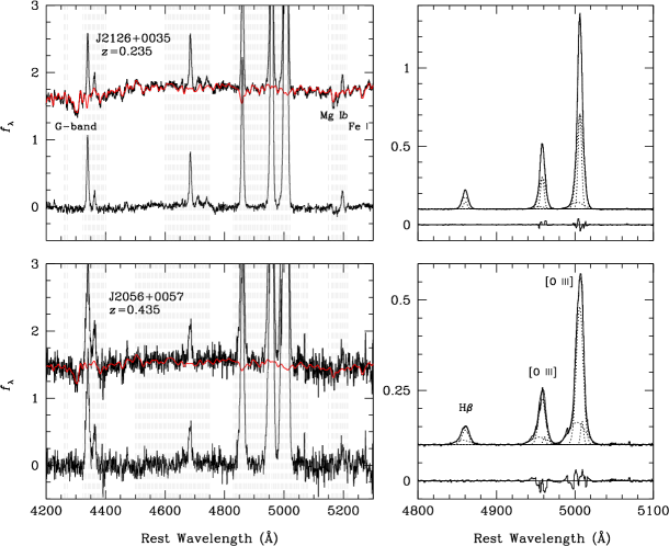
Figure 1: Example fits to two objects in the sample, spanning the range of redshift and S/N in the sample. Left: Stellar velocity dispersion fits using the best weighted fit of an F2, G5, K1, and K4 star. We plot LDSS3 spectra (thick histogram), best-fit model (red solid), and residuals (thin histogram). Data and models are offset for clarity, while regions excluded from the fit are demarcated with grey hatched lines. These fits provide both a measurements of $\sigma_{\ast}$ and a continuum-subtracted spectrum. Flux density is normalized to the continuum. Right: Fits to the H$\beta$ and [O III] emission lines using multi-component Gaussians; see text for details. Total model (thin solid) and model components (dotted) are plotted over the continuum-subtracted data (thick histogram). Residuals are offset for clarity and flux density is in units of $10^{-15}$ erg s^-1 cm^-2 Å^-1.

LDSS3, particularly during the March 2007 observation period, had intermittent but substantial pattern noise. Pattern noise appears as periodic striping in the data, with a typical scale of a few pixels and an amplitude (in these data) of 50–100 counts. The amplitude and phase vary in time and so standard calibrations do not remove it but there is a COSMOS task that Fourier transforms the data and removes the high-frequency noise. Our concern is that the frequency of the pattern noise is comparable in scale to that of the expected stellar velocity dispersions, potentially leading to biases in our final measurements. In order to test this possibility, we have performed three independent pattern-noise removal runs for the first night, which has particularly bad pattern noise. We have measured the dispersions independently for each of these spectra. The rms in the measured $\sigma_{\ast}$ values for the four objects range from 3 to 20 km s^-1, and, most crucially, we see no systematic differences in the measured dispersion for different versions of the pattern-noise removal. We conservatively add an additional 20 km s^-1 uncertainty in quadrature to the measured dispersions that suffer from pattern noise.

3 Stellar Velocity Dispersions

One of the primary uncertainties in interpreting observations of narrow-line quasars comes from their unknown BH masses. For the median $L_{\mathrm{[O{\tiny III}]}}$$=2\times 10^{42}$ erg s^-1 of the Magellan sample, we estimate that the bolometric luminosity is $L_{\rm bol}\approx 2\times 10^{45}$ erg s^-1, which suggests BH masses of $>10^{7}$ $M_{\odot}$ if they emit at or below their Eddington limits [where we take the Eddington luminosity to be $1.26\times 10^{38}$ ($M_{\mathrm{BH}}$/$M_{\odot}$) erg s^-1]. However, given the scatter between [O III] and bolometric luminosity, the range of bolometric luminosities in the sample, and their (presumed) range of intrinsic Eddington ratios, it would be nice to have an independent estimate of the BH masses. At the same time, it would be very useful to have a mass scale for the host galaxies. Although it is indirect, if we assume that the $M_{\mathrm{BH}}-\sigma_{\ast}$ relation holds, then we can use measurements of bulge velocity dispersions both to provide an estimate of the BH masses in the sample and as a proxy for the mass of the host galaxy (e.g., Heckman et al., 2004). Here we describe the $\sigma_{\ast}$ measurements and uncertainties; the BH masses are presented in §5.

There are a variety of commonly used techniques for measuring stellar velocity dispersions in galaxies. For computational expediency, most of them rely on Fourier techniques, including cross-correlation (Tonry & Davis, 1979), the Fourier quotient method (Simkin, 1974; Sargent et al., 1977), and the Fourier correlation quotient (Bender, 1990). It is also possible to directly compare broadened templates with data in pixel space (e.g.,  Burbidge et al., 1961). Direct-pixel fitting methods, while relatively computationally expensive, provide many benefits over Fourier techniques (e.g.,  Rix & White, 1992; van der Marel, 1994; Kelson et al., 2000; Barth et al., 2002; Bernardi et al., 2003), including the ability both to fit over restricted regions and to mask complicating emission or absorption features. As described in detail in Greene & Ho (2006), even faint emission lines can lead to substantial biases in derived $\sigma_{\ast}$ measurements if not properly accounted for.

Our galaxy models are built from a linear combination of stellar spectra. The program object is de-redshifted using the SDSS redshift, but inevitably small velocity shifts are present between the templates

and the target. Thus, each template is shifted to zero velocity, diluted by a constant or power-law component $C(\lambda)$, convolved with a Gaussian $G(\lambda)$, and multiplied by a polynomial $P(\lambda)$:

$$M(\lambda)=P(\lambda)\{[T(\lambda)\otimes G(\lambda)]+C(\lambda)\}$$ (1)

The nonlinear Levenberg-Marquardt algorithm, as implemented by mpfit in IDL (Markwardt, 2009), is used to minimize $\chi^{2}$ in pixel space between the galaxy and the model. Our code is based on that presented in Greene & Ho (2006), except that the model spectrum is actually a linear combination of stars (typically four in this work) with their relative amplitudes as additional free parameters. This version of the code was developed to model the high-quality nuclear spectra from the Palomar spectroscopic survey of nearby galaxies (Ho et al., 1995) and is presented and extensively tested in Ho et al. (2009). Unless otherwise noted we have used the following four stars as our template set: HD 26574 (F2 III), HD 107950 (G5 III), HD 18322 (K1 III), and HD 131507 (K4 III). Example fits are shown in Figure 1. While the primary purpose of the multi-template fitting is to achieve reliable fits, we also extract crude stellar population information in §7.

In order to use the full spectral range of the observations, we cannot rely only on our own template stars, whose wavelength coverage does not go blueward of $\sim$4300 Å. Rather, we utilize a large library of high-S/N, high-spectral resolution ($\sim 26$ km s^-1) stellar templates from Valdes et al. (2004). It is best to use template stars observed with an identical instrumental setup as the targets, so that the measured broadening can be ascribed solely to internal kinematics in the galaxy. However, the Valdes templates not only allow us to include spectral features such as the G-band $\lambda 4304$ Å to the highest redshifts, but also provide a wide range of spectral types to help minimize the impact of template mismatch. We thus use a simple bootstrapping procedure to remove the impact of differing instrumental resolutions on the measured dispersions. First of all, we measure the intrinsic broadening of the

Comparison of stellar velocity dispersion measurements using our internal velocity template stars ($\sigma_{\rm Our}$) and the Valdes template stars ($\sigma_{\rm Valdes}$) for the low-redshift targets. The template stars, while not identical, are matched exactly in spectral type to remove ambiguity caused by template mismatch. The measured dispersions from the Valdes templates are corrected for resolution assuming that the instrumental resolution of our LDSS3 measurements is $\sigma$=67 km s^-1, while the instrumental resolution of the Valdes stars is $\sigma$=26 km s^-1. As demonstrated here, the agreement is excellent, which supports our assumed conversion factor.

LDSS3 template stars using the Valdes library. While we did not observe identical stars, we can match the stars in spectral type nearly exactly. We expect the relative broadening to be $\sigma_{\rm rel}=(\sigma^{2}_{\rm LDSS3}-\sigma^{2}_{\rm Valdes})^{0.5}=(67^{2}-26^{2})^{0.5}=62$ km s^-1. We measure a mean broadening over 10 stars of 60$\pm$7 km s^-1. Dividing the sample into the two runs demonstrates the stability of the spectrograph; we find 61$\pm$8 km s^-1 and 59$\pm$7 km s^-1, respectively. Here and throughout, when we quote errors on mean quantities, we are quoting the standard deviation of the distribution rather than the error on the mean.

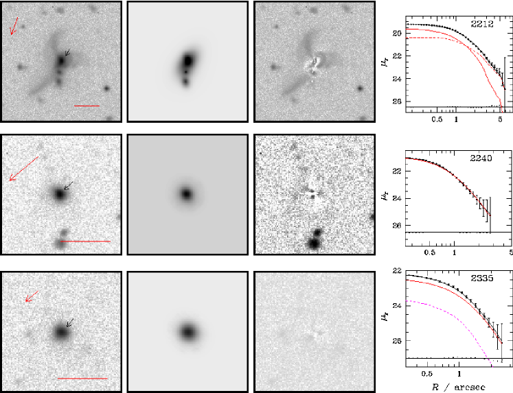
Figure 2: Fits are shown for each galaxy, with the exception of J1124 and J1142, for which the PSF is too poor to use the images. Scale bar indicates 10″, red arrow points North, and black arrow points to the main target. We show the LDSS3 image (left), the best-fit GALFIT model (middle) and the two-dimensional residuals (right), and then the one-dimensional radial profile. The points are the data, the red lines are the bulge components, the blue solid line is the disk component, the magenta solid line shows a bar component, and magenta dotted line is the PSF. The green lines are additional $n=2$ Sérsic components in J1356, which is too disturbed to be well fit by azimuthally symmetric models such as these. The one-dimensional residuals are shown at the bottom. The magenta dotted line in J2335 represents an unresolved nuclear component. Note that J0157 is in the wings of a very bright star, making the fitting very uncertain. The sharp features present in the models of J0157 and J1507 are due to the artificial truncation of the PSF model. Finally, in J1106, we compare the ellipse profiles for the HST-ACS FR647M ($\lambda_{\rm c}=7210$ Å; magenta points) and F550M ($\lambda_{\rm c}=5581$ Å; green points) with the LDSS3 $r$-band image. Our bulge size may be contaminated by a prominent unresolved nuclear source presumably due to scattered light.

We then confirm that our conversion works properly by measuring the velocity dispersions of our targets with the Valdes templates and comparing the values to those measured from our internal templates, again being careful to match the spectral types of the template stars and the fitting regions. The resulting dispersions are shown in Figure 2, where the reported Valdes dispersions have been reduced by $60$ km s^-1 in quadrature. It appears that our conversion is quite robust. From now on we report results based entirely on the Valdes stars with the above correction, conservatively adding 7 km s^-1 in quadrature to our error budget. The resulting $\sigma_{\ast}$ measurements are shown in Table 2.

In the interest of uniformity, in all cases we use the spectral region 4100–5400 Å, which is accessible for every observation. We follow Greene & Ho (2006) and mask out the Mg I$b$ $\lambda\lambda 5167,5172,5183$ triplet. While the Mg I$b$ triplet is one of the highest equivalent width (EW) features in this spectral region, the well-known correlation between the [Mg/Fe] ratio and $\sigma_{\ast}$ (e.g., O‘Connell, 1976; Kuntschner et al., 2001) leads to a systematic overestimate of $\sigma_{\ast}$ based on Mg I$b$ (Barth et al., 2002).

Input-output simulations to estimate uncertainties in $\sigma_{\ast}$ resulting from the finite S/N and continuum dilution. $\Delta\sigma$$\equiv\langle\sigma_{\rm out}-\sigma_{\rm in}\rangle/\sigma_{\rm in}$. We investigate S/N=10 (solid black, circles), S/N=15 (blue short-dashed, triangles), and S/N=30 (red long-dashed, squares). In all cases, two-thirds of the continuum is a nonthermal component modeled as a constant. Each setting is run with 10 randomly generated error arrays. We see that there is no net offset even at these low S/N ratios and high dilution values, but uncertainties range from $\sim 10\%$ to 20%.

3.1 SDSS Spectra

In order to increase our sample size, we have also considered all of the targets in the Reyes et al. (2008) sample. Since most of the spectra do not have the required S/N for reliable velocity dispersion measurement, we have limited our attention to objects with a median S/N of $>$15 per pixel between 5080 and 5400 Å, and an EW in the Ca K line greater than 3 Å. There are 547 objects with $L_{\rm[O\tiny III]}>10^{42}$ erg s^-1; of those, 111 make our cut. The SDSS velocity dispersions are measured in an identical fashion as the fits described above, using the same mix of Valdes template stars. In this case, we assume an instrumental resolution of 71 km s^-1 for the SDSS spectra (see discussion in Greene & Ho, 2006).

The SDSS-derived $L_{\mathrm{[O{\tiny III}]}}$ values, our measured velocity dispersions, and [O III] line widths for this additional sample are all presented in Table 3. Two objects are unresolved ($\sigma_{\ast}$$<71$ km s^-1). There are only two objects from the Magellan sample for which we can measure reliable dispersions from the SDSS spectra, and the resulting dispersions agree with ours within the quoted uncertainties.

3.2 Uncertainties

Our quoted uncertainties are a quadrature sum of the formal errors from the fit and the 7 km s^-1 uncertainty incurred in converting to the Valdes system. Our typical uncertainties thus derived range from $10\%$ for the lower-redshift targets to $40\%$ for the most distant and luminous targets.

As the S/N in the spectrum decreases, our ability to recover the true dispersion decreases. Also, an increasing contribution to the continuum from sources apart from old stars lowers their EW and thus the S/N. To a small degree the relative incurred error also depends on the true dispersion.

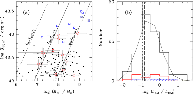
Figure 3: (a) Sample of narrow-line quasars from Reyes et al. (2008) above a luminosity threshold of $L_{\mathrm{[O{\tiny III}]}}$$=10^{42}$ erg s^-1 for which we were able to measure reliable $\sigma_{\ast}$ values. The BH masses are derived indirectly from $\sigma_{\ast}$, assuming the $M_{\mathrm{BH}}-\sigma_{\ast}$ relation of Tremaine et al. (2002), while the bolometric luminosities are derived indirectly from $L_{\mathrm{[O{\tiny III}]}}$. We show the Magellan sample (red open circles), the Gemini sample from Liu et al. (2009, ; blue open squares), and the SDSS sample (small filled circles). Double nuclei from the Gemini data are indicated with a cross. (b) The inferred distribution of Eddington ratios for the entire sample, with the Magellan data (red open), Gemini data (blue hatched) and best-fit Gaussian (thin solid) overplotted. We note that the uncertainties in this derivation are very large; 0.4 dex for the bolometric correction and 0.5 dex in $M_{\mathrm{BH}}$. Given such large uncertainties, the $L_{\mathrm{bol}}/L{\mathrm{{}_{Edd}}}$ distribution is strikingly narrow. The central values of the Kollmeier et al. (dashed), Gavignaud et al. (long dash), and Shen et al. (dash-dot) distributions are shown for comparison.

We run a suite of simulations designed to quantify each of these effects by adding Gaussian random noise and a constant continuum of various levels to one of the template stars that has been broadened to various widths. We create ten mock spectra for each S/N value, and then measure $\sigma_{\ast}$ for each mock spectrum. This simple input-output experiment shows that our error bars are reasonable. We expect $10\%-20\%$ errors for the targets with $10<S/N<30$ and $67\%$ continuum dilution (Fig. 3).

Systematic uncertainties may be introduced in the gas and stellar dispersions due to our use of fixed angular rather than physical apertures. In the case of the stars, we are typically extracting the spectra at $\sim 0.5~{}r_{\rm e}$. Since the velocity dispersion profiles of bulge-dominated galaxies are known to be flat (e.g., Jorgensen et al., 1995), in general aperture bias should be small compared to the measurement uncertainties. The only potential exceptions are the disk-dominated galaxies (J1106, J1222, and J1253) for which disk contamination may be significant. In the case of the gas, line widths can change dramatically as a function of aperture (typically getting narrower at large radius). Unfortunately, the dependence of gas dispersion on radius varies substantially from object to object (see, e.g.,  Rice et al., 2006; Walsh et al., 2008) and there is no physically motivated aperture to choose. In future work we will explore the full variation in gas velocity dispersion and luminosity as a function of radius.

3.3 Emission-line Fits to Nuclear Spectra

A convenient additional product of our velocity dispersion fits is a continuum-subtracted emission-line spectrum for each target. Since we are interested in the [O II] line when it falls in the bandpass, we extend the model out to the bluest available pixels although we do not use those wavelengths in the fitting. Examples of the continuum-subtracted spectra are shown in Figure 1, and we note that all spectra have been extracted with a 2$\farcs$25 aperture. We fit the H$\beta$, [O III], and [O II] lines with multi-component fits. Briefly, the [O III] $\lambda\lambda 4959,5007$ lines are modeled with identical sets of Gaussian components, where the centroid shifts are fixed to the laboratory value. The H$\beta$ line is fit with a combination of two Gaussians (but see §7 for an alternate fit). Our prescription follows that described in detail in Greene & Ho (2005a), except that unlike that work in general we require more than two components to adequately model the lines. Furthermore, we do not place any restrictions on the relative widths or strengths of the lines. The [O II] $\lambda\lambda 3726,3729$ lines are modeled with identical sets Gaussian components (usually two), and the line ratios in the doublet are fixed to one. This procedure is necessary to decouple true velocity dispersion from the small velocity separation of the two components of the doublet.

The line widths and strengths are shown in Table 4. The [O III] line is known to have an asymmetric profile, often with a prominent blue wing (e.g., Heckman et al., 1981). Greene & Ho (2005a) find that using a two-component fit and removing the blue wing results in a line width that better tracks $\sigma_{\ast}$. However, we find that in many cases a two-component model is not an adequate description of these lines. As shown by many authors (e.g., Greene & Ho, 2005a; Barth et al., 2008; Ho, 2009), the FWHM of the line is relatively free of bias from the velocity structure at the base of the line. Therefore, we simply take $\sigma_{\rm g}$=FWHM/2.35, as measured from our best-fit emission-line model.

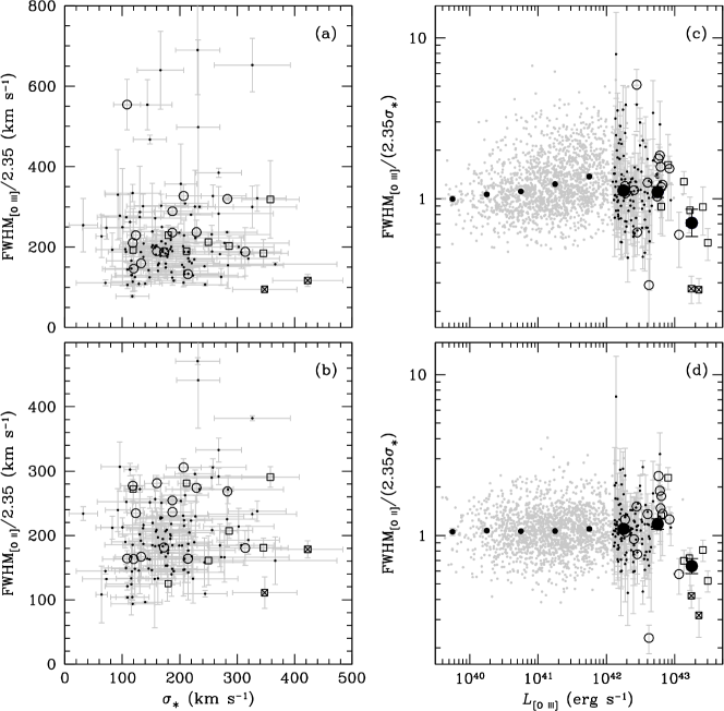
Figure 4: (a) Comparison of the velocity dispersion in warm gas as traced by the [O III] line to that of the stars. Following, e.g, Nelson & Whittle (1996) we plot the FWHM/2.35 for the gas versus the stellar velocity dispersion, also measured assuming a Gaussian broadening function (§3). We highlight the Magellan sample (open circles) and Gemini sample of Liu et al. (2009, ; open squares). Error bars in $\mathrm{FWHM}_{\mathrm{[O{\tiny III}]}}$ are dominated by deviations from the assumption of Gaussianity, determined by normalizing the measured full-width at 25% and 75% of maximum. (b) Same as (a) but using [O II] to measure the gas line width. (c) Dependence of the deviation of $\mathrm{FWHM}_{\mathrm{[O{\tiny III}]}}$ from $\sigma_{\ast}$ as a function of $L_{\mathrm{[O{\tiny III}]}}$. Formally there is no correlation. Symbols as above, but in grey we have added the lower-luminosity sample of Greene & Ho (2005a) to increase the dynamic range. Large filled circles show the median and standard error calculated in 0.5 dex bins for each subsample. There is no clear correlation between $\Delta\sigma$ and $L_{\rm[O{\tiny III}]}$ even over this large luminosity range. (d) Same as (c), but using $\mathrm{FWHM}_{\mathrm{[O{\tiny II}]}}$.

Although in the bulk of this paper we focus on the extractions with a 2$\farcs$25 aperture, we have made a variety of other extractions, with widths of 3$\farcs$78, 5$\farcs$67, and 7$\farcs$56. The last has an effective area comparable to the SDSS fiber (7 arcsec²). In Figure 4 we compare the $L_{\mathrm{[O{\tiny III}]}}$ measurements for our objects extracted (typically) within a 7$\farcs$56 aperture with the SDSS measurements. We find overall reasonable agreement, with $\langle\log L_{\rm[O{\tiny III}],SDSS}-\log L_{\rm[O{\tiny III}],our}\rangle=0.01\pm 0.2$. One object is a significant outlier; our measurement of J2212 is $\sim 6$ times fainter than that derived from the SDSS spectrum. This problem persists regardless of the flux calibrator used. It is curious, since we do not see a similar problem for any other target observed on this night. Since the discrepancy is seen in both the continuum level and the $L_{\mathrm{[O{\tiny III}]}}$ value, and since J2212 is a highly disturbed and spatially extended system (§4), we suspect that we were just unlucky in our slit placement and missed some luminous region of the galaxy. None of the conclusions presented here are impacted if we use the SDSS luminosity rather than ours. If we remove J2212, then the scatter between the two sets of measurements drops to 0.15 dex. We note that in our own observations $L_{\mathrm{[O{\tiny III}]}}$ can vary by as much as $80\%$ between different aperture positions, and so we are satisfied with this level of agreement.

4 Galaxy Structural Measurements

4.1 Photometric Zeropoints

We have also reduced the acquisition images (Table 1) using standard bias-subtraction and flat-fielding routines within IRAF. We do not attempt to remove the pattern noise in the images. Each frame is tied to the SDSS photometric system using three to six field stars. We use the IRAF package phot to perform aperture photometry on these relatively uncrowded fields, and then calculate a weighted average zeropoint based on the reported photometric errors in the SDSS photometry. The formal uncertainties in the final zeropoints are $<0.05$ mag.

4.2 Photometric Decomposition

The ground-based imaging reaches a typical surface brightness limit of $24-25$ mag arcsec^-2, and it is worth using the images to derive bulge-to-disk decompositions for the sample. Our goal is to isolate the bulge-like component of the host galaxy in order to compare with the Faber & Jackson (1976) relation of inactive bulge-dominated galaxies. The Faber-Jackson relation can provide a valuable diagnostic as to whether the galaxy has reached the relaxed state of local elliptical galaxies.

We use the two-dimensional surface brightness fitting program GALFIT (Peng et al., 2002) to model each galaxy. Our band of choice is Sloan $r$, since we have it for the majority of the targets. However, for various reasons we are forced in a few cases to model either the $g$- or $i$-band image.

Comparison of $L_{\mathrm{[O{\tiny III}]}}$ as measured from the SDSS spectra and our long-slit data with an aperture (typically) of 7$\farcs$56. The agreement is reasonable, with $\langle L_{\rm[O{\tiny III}],SDSS}-L_{\rm[O{\tiny III}],our}\rangle=0.01\pm 0.2$, and the scatter drops to 0.15 dex when the outlier (J2212) is excluded.

In these cases we convert to $r$ band using the measured color from the SDSS Petrosian magnitudes. Throughout, magnitudes are quoted in the AB system.

In comparison with broad-line AGNs the modeling is relatively straightforward in this case since there is no nuclear point source. As a rule, however, parameter coupling is a major complication (e.g., Kormendy & Djorgovski, 1989), and thus our operating principle is to model each galaxy with the minimum number of components. We are particularly interested in the bulge components of these galaxies, and we only introduce a disk component if visible in the images. In distinguishing between bulges and bars for disk-dominated galaxies we use the reduced $\chi^{2}$ to determine the preferred model, but we generally cannot constrain more than two galaxy components robustly. For the purposes of this paper we have not placed rigorous limits on the presence of low surface-brightness components (cf. Greene et al., 2008). Our basic model is the Sérsic (1968) function:

$$I(r)=I_{e}~{}{\rm exp}\left[-b_{n}\left(\frac{r}{r_{e}}\right)^{1/n}-1\right],$$ (2)

where $r_{e}$ is the effective (half-light) radius, $I_{e}$ is the intensity at $r_{e}$, $n$ is the Sérsic index, and $b_{n}$ is chosen such that

$$\int_{0}^{\infty}I(r)2\pi rdr=2\int_{0}^{r_{e}}I(r)2\pi rdr.$$ (3)

We adopt the analytic approximation for $b_{n}$ from MacArthur et al. (2004), as adapted from Ciotti & Bertin (1999):

$$b_{n}\approx 2n-\frac{1}{3}+\frac{4}{405n}+\frac{46}{25515n^{2}}+\frac{131}{1148175n^{3}}-\frac{2194697}{30690717750n^{4}}.$$ (4)

The Sérsic model reduces to an exponential profile for $n=1$ and a de Vaucouleurs (1948) profile for $n=4$. Bars may be modeled as ellipsoids with very low axial ratios. We follow de Jong (1996, ; see also  ) and model the intensity distribution in the bar as a Gaussian. In total for a given Sérsic component, the model parameters include the two-dimensional centroid, the total magnitude, the Sérsic index, the effective radius, the position angle, and the ellipticity (all of which are constants with radius for a given component in this version of GALFIT). The sky is modeled as a constant pedestal offset determined using multiple boxes placed in empty regions of the image, and Levenberg-Marquardt minimization of $\chi^{2}$ in pixel space is used for parameter estimation.

Even without a nuclear point source, proper modeling of the observed light distribution requires convolution with a PSF. We follow Ravindranath et al. (2006) and use Daophot as implemented within IRAF to build a PSF model, using no fewer than five isolated field stars on the same chip as the target galaxy. The PSF thus constructed is both noise-free and directly based on the PSF from the current image.

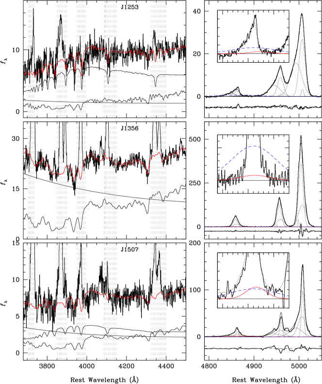
Figure 5: (Left) Three example fits used to constrain the blue-light fraction. We fit $3680-5400$ Å with a model including a K star, an A star, and a power law ($P_{\lambda}\propto\lambda^{-1.5}$), while $\sigma_{\ast}$ is fixed to our best fit from above. We plot the SDSS data (solid histogram), the best-fit model (red line), and model components (thin black solid line) as well as excluded regions (grey hatched). J1253 and J1507 contain a mixture of all three components, while J1356 requires only a K star and a (significant) power-law component. (Right) We show our best fits to the [O III]+H$\beta$ region of our LDSS3 spectra, with narrow H$\beta$ constrained to have the same shape as [O III]. We show the data (solid histogram), the total model (thin solid line), each model component (dash-dot line), the broad H$\beta$ component (red solid line), and the expected scattered broad component (blue dashed line). The latter assumes that all of the blue light is scattered, takes a standard conversion between H$\beta$ and $L_{\rm{5100\AA}}$ (Greene & Ho, 2005b), and assumes an H$\beta$ linewidth of 4000 km s^-1. In J1356 and J1253 there is evidence for recent star formation from the excess of blue light compared to the apparent broad component at H$\beta$, while J1507 can be explained purely with scattered light. Flux density in units of $10^{-17}$ erg s^-1 cm^-2 Å^-1.

Two-dimensional modeling provides a few advantages worth noting. For one thing, we gain the freedom to assign different position angles and (if necessary) centroids to different components (e.g., Wadadekar et al., 1999). Another major benefit of GALFIT for these galaxies, which often have nearby companions, is that we can simultaneously model the surrounding galaxies rather than mask them, which provides a considerably better model of the background. All fits are shown in Figure 5.

4.3 Uncertainties

Uncertainties in the measured parameters are driven primarily by the PSF model and the sky level, as well as inadequacies in the assumed model for the surface brightness profile. In order to estimate the former, we adopt a single star from the field as an additional PSF model. We further run a pair of models in which the sky level is increased and decreased by $0.5\%$, which is the typical dispersion in sky values across the field. The final error bars represent the dispersion in each parameter from these four alternate runs. Our methodology is described in more detail in Greene et al. (2008).

The hardest uncertainties to estimate arise when our assumed model is incorrect. Indeed, in J1356 and J2212 (see Table 2 and Fig. 5), the isophotes are so disturbed due to ongoing merging activity that we do not achieve a sensible fit from a simple combination of one or two Sérsic components. In these two cases, due to the presence of tidal features and spatially overlapping nuclei, our models are not particularly meaningful. Instead, we adopt a nonparametric Petrosian (1976) magnitude for clearly disturbed systems, as noted in Table 2. Furthermore, although the direct light from the active nucleus is extincted by many orders of magnitude, some of it escapes along unobscured directions, scatters off of the interstellar matter in the host galaxy and reaches the observer. Both our photometric modeling (see below) and spectroscopic fitting (§7) may be affected by this component. Finally, we do not have usable Magellan images for J1124 or J1142, and so we adopt SDSS magnitudes in Table 2.

As a sanity check, we compare our final galaxy luminosities to model magnitudes from SDSS, as well as to magnitudes from the HST survey of Zakamska et al. (2006) for overlapping galaxies. The total magnitudes we measure agree very well with the SDSS model magnitudes, with an average difference (ours$-$SDSS) of $0.005\pm 0.15$ mag, excluding J0157 because the photometry is exceedingly uncertain due to the proximity of a bright star. We are thus confident that our photometry is reasonable, but we adopt an additional 0.15 mag uncertainty in the bulge luminosities to account for the systematic differences between the two sets of measurements.

There are two objects in common between this paper and the HST sample, J1106 and J1413. Again, the total magnitudes agree reasonably well, within 0.07 mag in the case of J1106 and 0.4 mag in the case of J1413. (Color differences are derived from the LDSS3 spectra, and so strictly speaking only apply in the inner regions of the galaxy, and we account only for galactic extinction.) While we derive similar B/T ratios for J1106 from the two images, the derived bulge effective radii are different; we find $r_{e}=0.8\pm 0.4$ kpc, while it is found to be 3.8 kpc in the nearest HST band (F550M). The explanation for this difference can be seen in the radial profiles derived from the LDSS3 and HST images respectively (Fig. 5). A scattered-light component is detected in HST images as a biconical structure with a maximum extent of 0$\farcs$9 and appears as a central brightness peak in the one dimensional brightness profile. This component is not resolved with the LDSS3 images but may bias our derived bulge size to low values. At the same time, the strong dust lanes may mimic the transition between bulge and disk in the HST analysis, causing the HST bulge measurement to be too high. This one example emphasizes that we are potentially biased in our bulge sizes and luminosities due to scattered light. We do not detect the scattered light signal strongly in the spectrum, presumably because of internal reddening in the host galaxy.

4.4 Galaxy Morphology

In addition to reliable galaxy luminosities, we also have derived bulge-to-total ratios (B/T; Table 2) and general morphological information for this sample. There are four disk galaxies (J1106, J1222, J1253, and J2126) while the rest consist of a single bulge-like component, or in the case of J1356 and J2212, train-wrecks. Based on SDSS imaging, J1124 appears to be extended, but not obviously disky, while J1142 is compact. It is interesting to note, furthermore, that a large fraction of the sample have companions (eight out of 15, most confirmed with the long-slit spectroscopy). Four objects are significantly tidally disturbed, and thus obviously currently interacting (J0841, J1356, J1222, and J2212). There is no correlation between AGN luminosity or stellar velocity dispersion and galaxy morphology. Even if we include the HST observations of Zakamska et al. (2006), the median $L_{\mathrm{[O{\tiny III}]}}$ for objects with and without a disk component are identical to within 0.1 dex. On the other hand, the sample is quite small. Zakamska et al. (2008) find a hint that $L_{\mathrm{[O{\tiny III}]}}$ and morphology are correlated, in the sense that B/T decreases with AGN luminosity, but for objects extending to somewhat lower luminosities.

4.5 $k$-corrections and Stellar Populations

Our ultimate goal is to compare the structural properties of the narrow-line quasars to those of inactive galaxies, which involves translating our observations to match the exact observing procedures and evolutionary state of the local samples. Since our galaxies span a redshift range of $0.15<z<0.45$, we must assume a model of the intrinsic spectral shape in order to calculate an effective rest-frame luminosity. We use the publicly available program k-correct based on the SDSS photometry (Blanton & Roweis, 2007). It would be preferable to use the bulge component alone to derive the $k$-corrections, but given our heterogeneous coverage in different filters for different subsets of objects we use the SDSS photometry in the interest of uniformity.

Additionally, we must estimate the contamination from emission lines. These objects can have high EWs in [O III], meaning that the line emission contributes significantly to the broad-band luminosity. From $0.1<z<0.4$, [O III] contaminates the $r$-band magnitude, while at higher redshift it falls in the $i$ band. We calculate the total (extended) [O III] luminosity from our widest slit extraction, and convert to an AB magnitude using synphot in IRAF. The corrections thus derived, as well as the $k$-corrections for the corrected colors, are shown in Table 2.

Along the same lines, scattered light from the nucleus may contribute a sizable fraction of the luminosity in the blue. We have tried to disentangle contributions from both star formation and scattered light to the total luminosity (§7). Rerunning $k$-correct with the blue continuum removed leads to only $0.02-0.05$ mag of change in the final $k$-corrections. Finally, of course, stellar populations fade as they age, and the magnitude of that fading is dependent on the detailed star formation history of the galaxies in question. We will explore this last issue in §7.

5 Black Holes Masses and Eddington Ratios

It is hard to interpret observations of narrow-line AGNs in the absence of direct measurements of BH mass. The targets may be $10^{8}$ $M_{\odot}$ BHs radiating close to their Eddington luminosity or they may be more massive systems in a low accretion state. Their importance to the accretion history of the Universe, the interpretation of the observed properties of the host galaxies, and comparisons with broad-line objects all depend critically on the assumed mass scale. The stellar velocity dispersions and inferred range of BH masses thus constitute one of the main results of this paper.

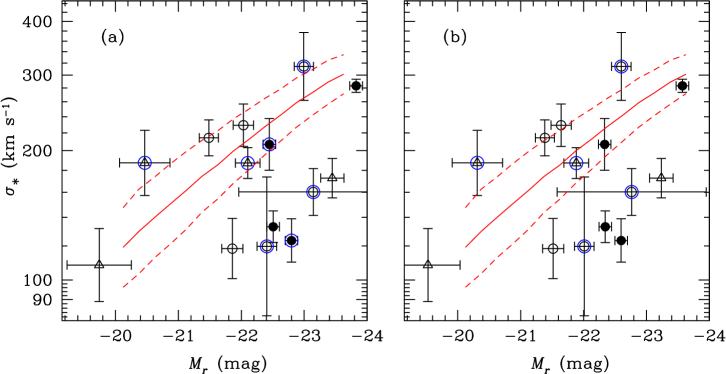
Figure 6: (a)Rest-frame $r$-band Faber-Jackson relation. We differentiate single $n>2$ profiles (open circles), bulge components of disk galaxies (triangles), and disturbed systems for which we use the nonparametric Petrosian magnitude (filled circles). Active galaxies with $L_{\mathrm{[O{\tiny III}]}}$$>10^{42.5}$ erg s^-1 are circled in blue. The inactive relation (red solid line), and uncertainties thereof (red dashed lines), are from Desroches et al. (2007), and are shown only over the region for which they were measured. (b) The same as (a) but with both a correction for the blue light (see text) and an evolution correction of 0.9$z$ mag.

Using the $M_{\mathrm{BH}}-\sigma_{\ast}$ relation of Tremaine et al. (2002), we convert $\sigma_{\ast}$ into BH mass and in Figure 6 we plot $M_{\mathrm{BH}}$ versus $L_{\mathrm{[O{\tiny III}]}}$ for the sample. Lines of constant Eddington ratio are highlighted, where the bolometric correction, ${\rm log}~{}L_{\rm bol}=0.99{\rm log}~{}L_{\rm[O{\tiny III}]}+3.5$ is taken from Liu et al. (2009). This correction is derived in two steps. First, the conversion between $L_{\mathrm{[O{\tiny III}]}}$ and $L_{\rm{5100\AA}}$ is calibrated using SDSS broad-line AGNs (Reyes et al., 2008), and then the relation between $L_{\rm{5100\AA}}$ and bolometric luminosity is derived based on two recent compilations of spectral energy distributions (SEDs), Marconi et al. (2004) and Richards et al. (2006). In the latter case, we have extrapolated the UV-optical slope downward beyond the near-infrared minimum in order to estimate the full contribution of the big blue bump, but exclude the reradiated mid-infrared emission. The estimated scatter is 0.4 dex, accounting for the 0.2 dex systematic difference between the two chosen bolometric corrections, the 0.36 dex scatter between $L_{\mathrm{[O{\tiny III}]}}$ and continuum luminosity in broad-line objects, and the 0.05 dex scatter in the single-band bolometric correction from Marconi et al. (Liu et al., 2009).

As seen in Figure 6, our narrow-line quasars appear to span $\sim 2$ dex in BH mass, luminosity, and Eddington ratio. Nominally, the Eddington ratios cluster around the value log $L_{\mathrm{bol}}/L{\mathrm{{}_{Edd}}}$$=-0.7$ with a dispersion of 0.7 dex (see the best-fit Gaussian fit to the distribution in Figure 6b), but it is important to bear in mind how the Eddington ratios are obtained. As was mentioned above, there is an 0.4 dex uncertainty in the conversion from $L_{\mathrm{[O{\tiny III}]}}$ to $L_{\rm bol}$. Furthermore, there is a $\sim 0.5$ dex uncertainty associated with each $M_{\mathrm{BH}}$ measurement which arises from the uncertainty in the velocity dispersion. Therefore, the observations are consistent with a population of sources radiating close to their Eddington luminosities, with the distribution of Eddington ratios broadened only by observational uncertainty.

Now let us compare our observations with the masses and Eddington ratios found for broad-line AGNs at similar redshifts. Kollmeier et al. (2006) find a strikingly narrow range in Eddington ratio for luminous broad-line AGNs at $0.3<z<4$. Shen et al. (2008) and Gavignaud et al. (2008) report similar results, although the latter paper finds evidence for an increased spread in $L_{\mathrm{bol}}/L{\mathrm{{}_{Edd}}}$ at lower luminosity. It appears that our sample is consistent with a similar behavior: rather than spanning a wide range in accretion rate, the objects are clustered close to their Eddington limits. At face value, not only do the narrow- and broad-line objects share comparable space-densities at the same luminosity (Reyes et al., 2008), but their distributions of mass and Eddington ratio are also surprisingly similar. Probably our application of a luminosity threshold is partially responsible for the observed narrow distribution in BH mass. The Eddington limit effectively determines the lowest-mass BHs to be included in the sample, while the space density of high-mass BHs declines exponentially (e.g., Hopkins et al., 2009). Nevertheless, while a variety of correlated errors or selection effects may contribute to the apparent narrow distributions observed in each population, the point we emphasize here is that the selections and biases are quite different between the broad and narrow-line objects, and thus the similarity in derived distributions is surprising.

There are several steps involved in calculating $M_{\mathrm{BH}}$ and $L_{\mathrm{bol}}/L{\mathrm{{}_{Edd}}}$, each of which has the potential to introduce systematic biases into the measurements. First, there is still substantial disagreement about the calculation of $M_{\mathrm{BH}}$ in broad-line quasars on the basis of continuum luminosity and broad line width (e.g., Baskin & Laor, 2005; Collin et al., 2006; Gavignaud et al., 2008; Shen et al., 2008). Second, the bolometric luminosity correction for narrow-line quasars uses a conversion from $L_{\mathrm{[O{\tiny III}]}}$ to $M_{\rm B}$ derived for broad-line quasars, and this procedure may systematically bias the bolometric luminosities towards low values (Netzer et al., 2006; Reyes et al., 2008). Furthermore, one may question our assumption that the $M_{\mathrm{BH}}-\sigma_{\ast}$ relation holds for narrow-line quasars. For one thing, they are active (i.e., currently accreting) BHs and thus may be offset from the local relation (Ho et al., 2008; Kim et al., 2008). In addition, there may or may not be significant redshift evolution of the local $M_{\mathrm{BH}}-\sigma_{\ast}$ relation that we use to calculate $M_{\mathrm{BH}}$, and both the sign and the magnitude of this change are at present unknown (Woo et al., 2006; Peng et al., 2006a, b; Treu et al., 2007; Lauer et al., 2007). Each of these effects may potentially bias the calculation of Eddington ratios by as much as 0.5 dex. The similarity of Eddington ratios of broad- and narrow-line quasars, as well as the narrowness of their distribution, is an interesting and suggestive result, but we caution that some systematic effects may be affecting the comparison.

6 Comparison of Stellar and Gaseous Kinematics

It has long been known that the [O III] line width traces the bulge velocity dispersion in low-luminosity AGNs (e.g., Heckman et al., 1981; Whittle, 1992a, b; Nelson & Whittle, 1996). Recently, with the discovery of the $M_{\mathrm{BH}}-\sigma_{\ast}$ relation (Gebhardt et al., 2000; Ferrarese & Merritt, 2000), interest in the gas velocity dispersion ($\sigma_{\rm g}$) has increased, due to the possibility of using it as a proxy for $\sigma_{\ast}$ in distant or luminous active galaxies for which it is prohibitive to measure $\sigma_{\ast}$ directly (e.g., Nelson, 2000; Wang & Lu, 2001; Boroson, 2002; Shields et al., 2003; Grupe & Mathur, 2004; Onken et al., 2004; Greene & Ho, 2005a; Rice et al., 2006; Salviander et al., 2007). As a result, it becomes all the more crucial to understand the physical origin of the observed correlation, and to characterize whether it depends on properties of the AGN, such as bolometric luminosity, Eddington ratio or radio luminosity. This work increases the luminosity range over which such comparisons have been done by nearly two orders of magnitude, providing a crucial check of the assumption that $\sigma_{\ast}$$\approx$$\sigma_{\rm g}$. By the same token, given that $\sigma_{\rm g}$ and $\sigma_{\ast}$ have now been measured for large samples of weakly active galaxies over a wide range of Hubble types (Ho, 2009), it is possible to use the variations in this ratio as a probe of the impact of the AGN on the surrounding interstellar medium (ISM).

As shown in Figure 7, there appears to be no correlation between either $\mathrm{FWHM}_{\mathrm{[O{\tiny III}]}}$ or $\mathrm{FWHM}_{\mathrm{[O{\tiny II}]}}$ and $\sigma_{\ast}$ at these high luminosities (the Spearman correlation coefficient is $\rho=0.07$ with a probability $P=0.4$ that no correlation is present). We note that while we span a narrow range in luminosity, we actually span a wide range in $\sigma_{\ast}$, suggesting that the lack of correlation is a generic property of luminous obscured AGNs, and may well be a generic property of all AGNs at such high luminosities. We try to salvage the correlation by relying on lines with lower ionization potential, since many studies have found systematic trends between line shape and the critical density or ionization potential of the lines (e.g., Pelat et al., 1981; Filippenko & Halpern, 1984; Filippenko, 1985; De Robertis & Osterbrock, 1986). Generically speaking the high-ionization and/or high-critical density lines originate from closer to the BH and are thus typically broader, making low-ionization lines a better choice as proxies to $\sigma_{\ast}$ (e.g., Greene & Ho, 2005a; Komossa & Xu, 2007). Instead, we find that the [O II] and [O III] gas widths are strongly correlated ($\rho=0.9$, $P=10^{-5}$; $\mathrm{FWHM}_{\mathrm{[O{\tiny II}]}}$/$\mathrm{FWHM}_{\mathrm{[O{\tiny III}]}}$$=1.0\pm 0.2$), but neither correlates well with $\sigma_{\ast}$.

In search of some physical insight into the processes driving the gas dispersion, we explore correlations between various AGN properties and $\sigma_{\rm g}$/$\sigma_{\ast}$. For convenience, we define the logarithmic difference $\Delta\sigma$$\equiv$log $\sigma_{\rm g}$$-$log $\sigma_{\ast}$. Within the sample as a whole, $\langle$$\Delta\sigma$$\rangle=0.04\pm 0.2$. This is to be compared with $\langle$$\Delta\sigma$$\rangle=-0.15\pm 0.22$ for low-luminosity AGNs in early-type galaxies (Ho, 2009) and $\langle$$\Delta\sigma$$\rangle=0\pm 0.46$ for local narrow-line AGNs from SDSS (Greene & Ho, 2005a). Historically, many papers have found a correlation between radio power and [O III] line width (e.g., Wilson & Willis, 1980; Whittle, 1992a, b; Nelson & Whittle, 1996). We see no evidence for increasing $\Delta\sigma$ or $\sigma_{\rm g}$ with increasing radio power over a range of $10^{22}<L_{R}$/W Hz^-1$<10^{25}$ at 1.4 GHz. The Nelson & Whittle sample does extend an order of magnitude higher in radio luminosity, but it is clear that jets alone cannot explain the sources with very large gas dispersions (see also Greene & Ho, 2005a; Ho, 2009). According to Ho (2009), the deviation of $\sigma_{\rm g}$ from $\sigma_{\ast}$ shows a clear dependence on AGN luminosity and Eddington ratio (see also Greene & Ho, 2005a), in the sense that more luminous AGNs have a larger $\sigma_{\rm g}$/$\sigma_{\ast}$ ratio on average. We see no statistically significant correlation between $L_{\mathrm{[O{\tiny III}]}}$ and $\Delta\sigma$ ($\rho=-0.1$, $P=0.2$). Granted, the dynamic range in luminosity is very narrow for this sample alone, but, if anything, there is a weak negative trend of $\Delta\sigma$ with luminosity. Indeed, the lower-luminosity data from Greene & Ho (2005a) shown in Figure 7cd clearly demonstrate that there is not a well-defined correlation between $\Delta\sigma$ and $L_{\mathrm{[O{\tiny III}]}}$ over a much larger luminosity range.

While these results are discouraging in terms of the use of $\mathrm{FWHM}_{\mathrm{[O{\tiny III}]}}$ to approximate $\sigma_{\ast}$, they do tell us in no uncertain terms that the ISM in the hosts of these luminous quasars is very disturbed. As mentioned above, gas line widths in the centers of inactive and weakly active galaxies are well-described by virial or slightly sub-virial motions due to turbulence (Ho, 2009). In low-luminosity active galaxies, there is some evidence that AGN activity is, on average, increasing the gas line widths (Greene & Ho, 2005a; Ho, 2009), but overall the gas still appears to be dominated by virial motion, at least in a luminosity-weighted sense. In stark contrast, at the highest AGN luminosities, we see no correlation of gas and stellar velocity dispersions, suggesting that the ISM is completely disturbed.

7 Coincidence of Star Formation and Black Hole Growth

Despite decades of research, the prevalence of temporally coincident star formation and accretion remains one of the outstanding problems in AGN physics (e.g., Boroson & Oke, 1984; Heckman et al., 1995; Canalizo & Stockton, 2001; Kauffmann et al., 2003b; Ho, 2005a). Generically speaking, it seems difficult to inhibit star formation when there is a large enough gas supply to fuel a luminous AGN. On the other hand, robust measurements of star formation are difficult to obtain, particularly with a luminous broad-line AGN spilling light in all directions and at all wavelengths. Our hope is to gain new insights from the study of obscured but intrinsically quite luminous accreting BHs.

Of course, there are always complications. In our case, although the primary emission from the AGN is obscured, nevertheless accretion luminosity manages to contaminate many standard star formation indicators. The most reliable instantaneous (i.e. $<10^{7}$ yr) rate diagnostic, H$\alpha$ luminosity (e.g., Kennicutt, 1998), is excited by accretion power rather than young stars in our case. Likewise, blue/UV light is prone to contamination from scattered AGN light, whose magnitude can be very significant at these high luminosities (e.g., Heckman et al., 1995; Zakamska et al., 2005, 2006; Young et al., 2009; Liu et al., 2009). In what follows we show that all of our galaxies are bluer than their inactive counterparts, and we use a variety of indirect techniques to disentangle the young starlight from scattered AGN light.

We begin by modeling the SDSS colors using stellar population synthesis techniques. As input, we use the SDSS $ugriz$ magnitudes, with the [O III] and $k$-corrections applied, as described in §4.3. We do not apply any correction for potential scattered light, as our goal is to establish whether or not there is a blue component apparent in the integrated colors of the galaxies. The stellar population synthesis code is described in detail in Conroy et al. (2009). In short, the code utilizes isochrones from Padova (Marigo & Girardi, 2007), the BaSeL3.1 stellar libraries with thermally pulsating asymptotic branch stars added (Lejeune et al., 1997, 1998; Westera et al., 2002), and (in this case) a Kroupa (2001) initial mass function. Dust attenuation optical depths are allowed to vary separately for old and young stars, following the model of Charlot & Fall (2000).

The D_n(4000) and H$\delta_{\rm A}$ indices measured from our continuum fits (see text for details). The locus of points from Kauffmann et al. (2003a) is shown in contours, while our measurements are the overplotted red crosses. Stellar age increases towards the bottom right of the diagram. The top histogram shows the distribution of D_n(4000) from the spectra themselves corrected for [Ne III], but not corrected for the blue power-law component while the points are derived from the spectral modeling.

The fraction of total stellar mass formed in the last 300 Myr for each galaxy is shown in Table 4, with a median value of $1\%$ at a median stellar mass of $10^{11}$ $M_{\odot}$. Already we see that while the BHs are experiencing a major growth episode, the galaxies are not.

The integrated colors show that blue light is prevalent, but spectroscopy is required to determine its origin. For the purpose of comparing with Kauffmann et al. (2003a), we measure the D_n(4000) and H$\delta_{\rm A}$ indices. This two-dimensional diagnostic is predominantly sensitive to age, and relatively insensitive to variations in metallicity or dust. We follow their conventions, wherein D_n(4000) is defined as the ratio of fluxes in bands at 3850–3950 and 4000–4100 Å (Balogh et al., 1999), and H$\delta_{\rm A}$ is defined in Worthey & Ottaviani (1997). As a function of age, galaxies follow a well-defined sequence in D_n(4000)-H$\delta_{\rm A}$ space, and the locus of SDSS galaxies in this space is shown in Figure 8. Unfortunately, because our AGN-powered emission lines have such high EWs, we cannot measure a meaningful H$\delta_{\rm A}$ index directly from the spectra. We can measure D_n(4000) after correcting for [Ne III]$~{}\lambda 3869$, and those values are shown in the top histogram in Figure 8. [We have verified that we can reproduce the values in Kauffmann et al. Measuring the 30 most luminous objects in their DR2 catalog, we find $\langle$[D_n(4000)_our-D_n(4000)_Kauff]/D_n(4000)${}_{\rm Kauff}\rangle=-0.04\pm 0.05$.] The median of our sample, uncorrected for any blue component, is $\langle$D_n(4000)$\rangle=1.2$. For comparison, the thirty most luminous targets in the Kauffmann et al. DR2 sample, with a median $L_{\mathrm{[O{\tiny III}]}}$ of $10^{42}$ erg s^-1 ($\sim 0.5$ dex less luminous than our median luminosity), have $\langle$D_n(4000)$\rangle=1.3$.

Our first task is to measure the luminosity of the blue continuum. The LDSS3 spectra do not always include the 4000 Å break, and so we use the SDSS spectra for this measurement. We wish to model the various spectral components, but to mitigate degeneracy we restrict the model to nothing more than a K star, an A star, and a blue power law whose slope is fixed to $P_{\lambda}\propto\lambda^{-1}$. In principle the slope of the blue component will depend on the physical process responsible for it; given the modeling degeneracies and the uncertainties in internal reddening and flux calibration, we do not attempt to measure the true spectral shape of the blue light. Likewise $\sigma_{\ast}$ is fixed to the best-fit value determined in §3. While the fits are not unique, we believe each component is reasonably well constrained: a significant A or F star contribution is fixed by higher-order Balmer absorption lines, while the EW of the old stellar component provides a direct probe of the dilution by blue light. By repeating the fitting with a power-law slope of $-1.5$, we confirm that the derived luminosities are insensitive to the assumed power-law slope. More reassuringly, fits performed without an A star component yield blue luminosities that agree within 0.05 dex of the nominal result.

These fits provide two useful measurements: one is a blue luminosity, and the other is a (model-dependent) measurement of the D_n(4000) and H$\delta_{\rm A}$ indices for the underlying stellar population, as shown by red crosses in Figure 8. The stellar population gets older as one moves to the lower right of this diagram. Note that three objects have D_n(4000) indices that are larger than values seen in real galaxies. Presumably the discrepancy arises because in these cases the stellar continuum is modeled by a single K star, whereas in real stellar populations there will be some contribution from M stars as well as younger populations. The D_n(4000) and H$\delta_{\rm A}$ indices derived this way represent a lower limit on the young population, while below we will attempt to evaluate what fraction of the blue light may originate in young stars.

If the blue light is predominantly scattered AGN light, we can predict the corresponding reflected broad H$\beta$ component, using the well-known tight correlation between optical/UV continuum luminosity and Balmer emission (e.g., Searle & Sargent, 1968); we use the recent calibration of Greene & Ho (2005b). The expected line fluxes are low ($\sim 10^{-16}$ erg s^-1 cm^-2), but we can at least determine whether or not our spectra are consistent with a broad component at this level. In the most luminous narrow-line quasars, Liu et al. (2009) robustly detect a broad H$\beta$ component in a significant fraction of their sample and determine the scattered light contribution to the blue continuum (see also Terlevich et al., 1990; Heckman et al., 1995; Cid Fernandes et al., 2004). Here, because the lines are much weaker, we rather take the indirect approach of comparing the expected scattered emission from the continuum fits with a direct fit to the H$\beta$ line. If the two H$\beta$ fluxes are consistent, then we conclude that the blue light may be ascribed exclusively to scattered light.

Since the narrow-line shapes are quite complex and highly non-Gaussian, care must be taken to ensure that structure in the narrow lines does not masquerade as a bona fide scattered broad component. We thus repeat the narrow-line fits as described above, except that in this case we fix the narrow components of H$\beta$ to that of [O III], and allow the fit to include an additional broad H$\beta$ component. We constrain $3000<$FWHM${}_{\rm H\beta}<6000$ km s^-1 (Liu et al. find H$\beta$${}_{\rm FWHM}\approx 4000$ km s^-1), since otherwise the broad line will often attempt to fit low-level wiggles in the continuum.

In all cases the [O III] and H$\beta$ line shapes match each other extremely well (Fig. 9), and in eight cases we detect a broad component (Table 4; Fig. 9 bottom). We convert the rms residuals into an upper limit on broad H$\beta$ assuming a FWHM of 4000 km s^-1. We take as the upper limit on the scattered broad component either the detected broad H$\beta$ luminosity or the upper limit thereof, whichever is larger, and then compare with the luminosity we expect based on the detected blue continuum. If the two agree within a factor of 2, then we believe scattered light can fully account for the blue light, whereas when the continuum level is higher, we ascribe the excess to current star formation (the five cases are noted with * in Table 4).

When detected, the blue light accounts for anywhere from 5% to 60% of the total continuum flux at 4000 Å. After the blue light is removed, our galaxies occupy a sensible region of the H$\delta_{\rm A}$-D_n(4000) plane relative to the inactive galaxy population. The median D_n(4000) rises from 1.2 to 1.6. Even excluding those galaxies with D_n(4000) larger than what is seen in SDSS galaxies yields an average value of 1.5. In other words, while there is clearly an age spread, the corrected index values suggest that the galaxy light is dominated by old stellar populations in the majority of cases. In five galaxies (J0841, J1222, J1253, J1356, and J2212), we find a blue continuum in excess of what can be explained by scattered light, which we interpret as a star-forming component. It is interesting to note that these systems tend to have higher star formation rates inferred from their broad-band colors as well. Even more intriguing is the observation that all of the highly disturbed systems have an excess (star-forming) blue component. On the other hand, we see no correlation between the D_n(4000) values and host morphology. In summary, these host galaxies are forming $\lesssim 1\%$ of their stellar mass at the present time. About half of the objects are consistent with having only old stellar populations, while the others show evidence for ongoing (in the form of excess blue light) or recent [low values of D_n(4000)] star formation at a low level. While we cannot place absolute limits on the current star formation rate to any great precision, we argue here, and based on the structural parameters investigated below, that the galaxies are effectively fully formed.

In Figure 10 we show the $r$-band Faber-Jackson relation for the galaxy bulge components, with the most luminous targets circled in blue and the disk- or bulge-dominated galaxies differentiated as triangles or circles, respectively. Obviously there is a large amount of scatter in this diagram, much of it measurement-based. It appears that nearly half of the targets are offset toward more luminous bulges at a given $\sigma_{\ast}$, but we caution that there are substantial systematic biases hidden in the bulge luminosities, as discussed below.

We do not see any correlations between location in the Faber-Jackson diagram and AGN luminosity, young stars (as traced by the blue light), or intermediate-age stars [D_n(4000)]. Partly, the sample is just too small, spanning too narrow a range in luminosity, to display any such trends. At the same time, a number of potential uncertainties may impact the measured luminosities. There is firstly the contamination from scattered blue light, which boosts the observed $r$-band magnitudes by as much as 0.5 mag. Also, the targets span a range of redshifts ($0.1<z<0.45$), but we know that over time a collection of stars will become less luminous as the most massive stars evolve. Unfortunately, as shown by, for example, Conroy et al. (2009), the precise magnitude of this fading is highly uncertain (by $\sim 1$ magnitude), due to our inadequate knowledge of the slope of the initial mass function around the turnoff mass. Taking a value of 0.9$z$ mag in $r$ for the purposes of illustration (e.g.,  van Dokkum & Franx, 2001; Treu et al., 2005; Conroy et al., 2009), and removing the detected blue light yields the magenta points, substantially lowering the discrepancy with the local Faber-Jackson relation. We are reluctant to provide any additional interpretation, given the small sample and substantial uncertainties in the measurements.

Our basic conclusion, combining the results of the stellar population modeling, stellar population indices, and structural properties, is that for the most part the host galaxies had their stellar content in place prior to this epoch of substantial BH growth. The general result, that we see a range of star-forming properties with no clear correlation between host galaxy morphology and star formation properties, is in broad agreement with previous results for lower-luminosity narrow-line AGNs (e.g., Schmitt et al., 1999; González Delgado et al., 2001; Cid Fernandes et al., 2004).

Most interestingly, the situation appears rather different for objects at the highest luminosities. There, Liu et al. (2009) see clear evidence for Wolf-Rayet features in $\sim 1/3$ of their targets (we see none in this sample), which constitute a clear signature of a recent burst of star formation (e.g., Allen et al., 1976; Kunth & Sargent, 1981). Furthermore, Zakamska et al. (2008) find very high star formation rates from mid-infrared spectroscopy, for a different sample of luminous narrow-line AGNs, rates that are substantially higher than either those seen in inactive galaxies of similar mass or those in typical broad-line AGN samples of similar luminosity. Now, Kauffmann et al. (2003b) find compelling evidence that the post-starburst fraction increases with increasing [O III] luminosity. We may be seeing a hint that the galaxy growth rate scales with AGN luminosity even up to starbursts at the highest AGN luminosities (see also Canalizo & Stockton, 2001; Vanden Berk et al., 2006; Letawe et al., 2007; Jahnke et al., 2007).

HST images show that hosts of luminous narrow-line quasars from the SDSS-selected sample are bulge-dominated (Zakamska et al., 2005), whereas those of somewhat less luminous (by about 0.5 dex) IR-selected narrow-line quasars are dusty, disky systems (Lacy et al., 2007). This paper presents observations of objects with luminosities very similar to those in our HST sample, with similar results: about a third of the objects are found in strongly disturbed interacting systems, while the rest are found in bulge-dominated galaxies. We previously suggested that the difference in morphology may reflect the difference in the quasar fueling mechanisms as a function of quasar luminosity (Zakamska et al., 2008), but of course this interpretation is only tentative since the comparison samples were selected using very different methods. A detailed study of hosts of optically selected narrow-line quasars at lower luminosity is needed to understand the origin of the morphological difference.

8 Discussion and Summary

We have chosen to explore the host galaxy properties of obscured active galaxies in particular because of the increased contrast between galaxy and nucleus. On the other hand, it is our burden to determine whether or not our conclusions can be generalized to all accreting BHs at the epoch being probed. Rather surprisingly, the distributions of BH mass and Eddington ratio for our sample of narrow-line AGNs are quite similar to those seen in broad-line samples at similar luminosity and redshift (e.g., Kollmeier et al., 2006; Shen et al., 2008; Gavignaud et al., 2008). This fact, combined with the observation of Reyes et al. (2008) that the space densities of the broad- and narrow-line objects are comparable at fixed luminosity, suggest that the two may originate from similar populations. There is another aspect to the story, as illuminated by the differences in star-forming properties between the narrow- and broad-line objects.

A variety of recent papers have devised clever techniques for disentangling photoionization by stellar and nonstellar sources using the line strengths of high- and low-ionization lines, where the former are certainly dominated by the AGN but the latter can be significantly contaminated by star formation (e.g., Ho, 2005b; Kim et al., 2006; Villar-Martín et al., 2008; Meléndez et al., 2008). These studies all come to the same conclusion; star formation is more energetically significant in narrow-line than in broad-line AGNs, particularly at the luminous end (see also Zakamska et al., 2008). The excess star formation in narrow-line objects has been interpreted as evidence for an evolutionary scenario, in which obscured accretion and ongoing star formation coexist, and then accretion terminates further star formation, yielding an unobscured object (e.g., Sanders & Mirabel, 1996; Canalizo & Stockton, 2001; Ho, 2005b; Hopkins et al., 2006). In this picture some event (usually a merger) induces both the star formation and nuclear activity, and the broad-line object signifies the final stage in the accretion cycle.

Perhaps, on the other hand, there is not necessarily a causal connection between the star formation event and the accretion event, but when both occur simultaneously the odds are higher that the accretion event will be obscured by star formation in the host galaxy (Rigby et al., 2006; Lacy et al., 2007). Our data alone clearly cannot distinguish between these two possibilities. However, we do see a range of star formation properties across even this relatively small sample. Naively, if there were truly a causal connection between star formation and nuclear activity, one would expect that the majority of our sample would show a clear sign of ongoing star formation, even if only in the form of post-starburst signatures. We look forward to analyzing the full Reyes et al. (2008) sample to more definitively quantify the star formation properties as a function of AGN luminosity (Liu et al., 2009).

We have seen that luminous obscured active galaxies with $0.1<z<0.45$ and $10^{43}<L_{\rm bol}<10^{46.5}$ erg s^-1 are composed of BHs with masses $\sim 10^{8}$ $M_{\odot}$ radiating at a high fraction of their Eddington limits. We are seeing unambiguous evidence that BH accretion impacts the host on a galaxy-wide scale; the host galaxy ISM is clearly substantially disturbed relative to less active systems. As a result, we cannot recommend the use of gas line widths as a substitute for stellar velocity dispersions at such high luminosities, at least not in obscured sources. There is a clear blue component in the galaxies, apparent both in the overall colors and in nuclear spectroscopy, and in most cases the blue light is consistent with being scattered emission from the obscured nucleus. Nevertheless, nearly half of the sample shows evidence for recent or ongoing star formation, while the rest are consistent with predominantly old stellar populations. Although star formation activity may rise with vigorous AGN activity, there is a wide dispersion at all luminosities, suggesting that we are far from having a consistent picture of the coevolution of host galaxies and BH growth.

References

- Allen et al. (1976) Allen, D. A., Wright, A. E., & Goss, W. M. 1976, MNRAS, 177, 91
- Allington-Smith et al. (1994) Allington-Smith, J., et al. 1994, PASP, 106, 983
- Antonucci (1993) Antonucci, R. 1993, ARA&A, 31, 473
- Bahcall et al. (1997) Bahcall, J. N., Kirhakos, S., Saxe, D. H., & Schneider, D. P. 1997, ApJ, 479, 642
- Baldwin et al. (1981) Baldwin, J. A., Phillips, M. M., & Terlevich, R. 1981, PASP, 93, 5
- Balogh et al. (1999) Balogh, M. L., Morris, S. L., Yee, H. K. C., Carlberg, R. G., & Ellingson, E. 1999, ApJ, 527, 54
- Barth et al. (2008) Barth, A. J., Greene, J. E., & Ho, L. C. 2008, AJ, 136, 1179
- Barth et al. (2002) Barth, A. J., Ho, L. C., & Sargent, W. L. W. 2002, AJ, 124, 2607
- Baskin & Laor (2005) Baskin, A., & Laor, A. 2005, MNRAS, 356, 1029
- Bender (1990) Bender, R. 1990, A&A, 229, 441
- Bernardi et al. (2003) Bernardi, M., et al. 2003, AJ, 125, 1849
- Blanton & Roweis (2007) Blanton, M. R., & Roweis, S. 2007, AJ, 133, 734
- Boroson (2002) Boroson, T. A. 2002, ApJ, 565, 78
- Boroson & Oke (1984) Boroson, T. A., & Oke, J. B. 1984, ApJ, 281, 535
- Burbidge et al. (1961) Burbidge, E. M., Burbidge, G. R., & Fish, R. A. 1961, ApJ, 134, 251
- Canalizo & Stockton (2000) Canalizo, G., & Stockton, A. 2000, AJ, 120, 1750
- Canalizo & Stockton (2001) —. 2001, ApJ, 555, 719
- Charlot & Fall (2000) Charlot, S., & Fall, S. M. 2000, ApJ, 539, 718
- Cid Fernandes et al. (2004) Cid Fernandes, R., Gu, Q., Melnick, J., Terlevich, E., Terlevich, R., Kunth, D., Rodrigues Lacerda, R., & Joguet, B. 2004, MNRAS, 355, 273
- Ciotti & Bertin (1999) Ciotti, L., & Bertin, G. 1999, A&A, 352, 447
- Collin et al. (2006) Collin, S., Kawaguchi, T., Peterson, B. M., & Vestergaard, M. 2006, A&A, 456, 75
- Conroy et al. (2009) Conroy, C., Gunn, J. E., & White, M. 2009, ApJ, submitted (astro-ph/0809.4261)
- de Jong (1996) de Jong, R. S. 1996, A&A, 313, 45
- De Robertis & Osterbrock (1986) De Robertis, M. M., & Osterbrock, D. E. 1986, ApJ, 301, 727
- de Vaucouleurs (1948) de Vaucouleurs, G. 1948, Annales d’Astrophysique, 11, 247
- Desroches et al. (2007) Desroches, L.-B., Quataert, E., Ma, C.-P., & West, A. A. 2007, MNRAS, 377, 402
- Faber & Jackson (1976) Faber, S. M., & Jackson, R. E. 1976, ApJ, 204, 668
- Ferrarese & Merritt (2000) Ferrarese, L., & Merritt, D. 2000, ApJ, 539, L9
- Filippenko (1985) Filippenko, A. V. 1985, ApJ, 289, 475
- Filippenko & Halpern (1984) Filippenko, A. V., & Halpern, J. P. 1984, ApJ, 285, 458
- Freeman (1966) Freeman, K. C. 1966, MNRAS, 133, 47
- Gavignaud et al. (2008) Gavignaud, I., et al. 2008, A&A, 492, 637
- Gebhardt et al. (2000) Gebhardt, K., et al. 2000, ApJ, 539, L13
- González Delgado et al. (2001) González Delgado, R. M., Heckman, T., & Leitherer, C. 2001, ApJ, 546, 845
- Goodman (2003) Goodman, J. 2003, MNRAS, 339, 937
- Greene & Ho (2005a) Greene, J. E., & Ho, L. C. 2005a, ApJ, 627, 721
- Greene & Ho (2005b) —. 2005b, ApJ, 630, 122
- Greene & Ho (2006) —. 2006, ApJ, 641, 117
- Greene et al. (2008) Greene, J. E., Ho, L. C., & Barth, A. J. 2008, ApJ, 688, 159
- Grupe & Mathur (2004) Grupe, D., & Mathur, S. 2004, ApJ, 606, L41
- Heckman et al. (1995) Heckman, T., Krolik, J., Meurer, G., Calzetti, D., Kinney, A., Koratkar, A., Leitherer, C., Robert, C., & Wilson, A. 1995, ApJ, 452, 549
- Heckman et al. (1997) Heckman, T. M., Gonzalez-Delgado, R., Leitherer, C., Meurer, G. R., Krolik, J., Wilson, A. S., Koratkar, A., & Kinney, A. 1997, ApJ, 482, 114
- Heckman et al. (2004) Heckman, T. M., Kauffmann, G., Brinchmann, J., Charlot, S., Tremonti, C., & White, S. D. M. 2004, ApJ, 613, 109
- Heckman et al. (1981) Heckman, T. M., Miley, G. K., van Breugel, W. J. M., & Butcher, H. R. 1981, ApJ, 247, 403
- Ho (2005a) Ho, L. C. 2005a, preprint (astroph/0511157)
- Ho (2005b) —. 2005b, ApJ, 629, 680
- Ho (2009) —. 2009, ApJ, accepted
- Ho et al. (2008) Ho, L. C., Darling, J., & Greene, J. E. 2008, ApJ, 681, 128
- Ho et al. (1995) Ho, L. C., Filippenko, A. V., & Sargent, W. L. 1995, ApJS, 98, 477
- Ho et al. (2009) Ho, L. C., Greene, J. E., Filippenko, A. V., & Sargent, W. L. 2009, ApJ, submitted
- Hopkins et al. (2006) Hopkins, P. F., Hernquist, L., Cox, T. J., Di Matteo, T., Robertson, B., & Springel, V. 2006, ApJS, 163, 1
- Hopkins et al. (2009) Hopkins, P. F., Hickox, R., Quataert, E., & Hernquist, L. 2009, MNRAS, submitted (astroph/0901.2936)
- Horne (1986) Horne, K. 1986, PASP, 98, 609
- Jahnke et al. (2007) Jahnke, K., Wisotzki, L., Courbin, F., & Letawe, G. 2007, MNRAS, 378, 23
- Jorgensen et al. (1995) Jorgensen, I., Franx, M., & Kjaergaard, P. 1995, MNRAS, 276, 1341
- Kauffmann et al. (2003a) Kauffmann, G., et al. 2003a, MNRAS, 341, 33
- Kauffmann et al. (2003b) —. 2003b, MNRAS, 346, 1055
- Kelson (2003) Kelson, D. D. 2003, PASP, 115, 688
- Kelson et al. (2000) Kelson, D. D., Illingworth, G. D., van Dokkum, P. G., & Franx, M. 2000, ApJ, 531, 159
- Kennicutt (1998) Kennicutt, Jr., R. C. 1998, ARA&A, 36, 189
- Kim et al. (2006) Kim, M., Ho, L. C., & Im, M. 2006, ApJ, 642, 702
- Kim et al. (2008) Kim, M., Ho, L. C., Peng, C. Y., Barth, A. J., Im, M., Martini, P., & Nelson, C. H. 2008, ApJ, 687, 767
- Kollmeier et al. (2006) Kollmeier, J. A., et al. 2006, ApJ, 648, 128
- Komossa & Xu (2007) Komossa, S., & Xu, D. 2007, ApJ, 667, L33
- Kormendy & Djorgovski (1989) Kormendy, J., & Djorgovski, S. 1989, ARA&A, 27, 235
- Kormendy & Richstone (1995) Kormendy, J., & Richstone, D. 1995, ARA&A, 33, 581
- Kroupa (2001) Kroupa, P. 2001, MNRAS, 322, 231
- Kunth & Sargent (1981) Kunth, D., & Sargent, W. L. W. 1981, A&A, 101, L5
- Kuntschner et al. (2001) Kuntschner, H., Lucey, J. R., Smith, R. J., Hudson, M. J., & Davies, R. L. 2001, MNRAS, 323, 615
- Lacy et al. (2007) Lacy, M., Sajina, A., Petric, A. O., Seymour, N., Canalizo, G., Ridgway, S. E., Armus, L., & Storrie-Lombardi, L. J. 2007, ApJ, 669, L61
- Lauer et al. (2007) Lauer, T. R., Tremaine, S., Richstone, D., & Faber, S. M. 2007, ApJ, 670, 249
- Lejeune et al. (1997) Lejeune, T., Cuisinier, F., & Buser, R. 1997, A&AS, 125, 229
- Lejeune et al. (1998) —. 1998, A&AS, 130, 65
- Letawe et al. (2007) Letawe, G., Magain, P., Courbin, F., Jablonka, P., Jahnke, K., Meylan, G., & Wisotzki, L. 2007, MNRAS, 378, 83
- Liu et al. (2009) Liu, X., Zakamska, N. L., Greene, J. E., Strauss, M. A., Krolik, J. H., & Heckman, T. M. 2009, ApJ, submitted
- MacArthur et al. (2004) MacArthur, L. A., Courteau, S., Bell, E., & Holtzman, J. A. 2004, ApJS, 152, 175
- Marconi et al. (2004) Marconi, A., Risaliti, G., Gilli, R., Hunt, L. K., Maiolino, R., & Salvati, M. 2004, MNRAS, 351, 169
- Marigo & Girardi (2007) Marigo, P., & Girardi, L. 2007, A&A, 469, 239
- Markwardt (2009) Markwardt, C. B. 2009, ADASS 2008
- Martini (2004) Martini, P. 2004, in in Coevolution of Black Holes and Galaxies (Cambridge: Cambridge University Press), ed. L. C. Ho, 169–+
- Matheson et al. (2000) Matheson, T., Filippenko, A. V., Ho, L. C., Barth, A. J., & Leonard, D. C. 2000, AJ, 120, 1499
- Matheson et al. (2008) Matheson, T., et al. 2008, AJ, 135, 1598
- Meléndez et al. (2008) Meléndez, M., Kraemer, S. B., Schmitt, H. R., Crenshaw, D. M., Deo, R. P., Mushotzky, R. F., & Bruhweiler, F. C. 2008, ApJ, 689, 95
- Mihos & Hernquist (1994) Mihos, J. C., & Hernquist, L. 1994, ApJ, 431, L9
- Nelson (2000) Nelson, C. H. 2000, ApJ, 544, L91
- Nelson & Whittle (1996) Nelson, C. H., & Whittle, M. 1996, ApJ, 465, 96
- Netzer et al. (2006) Netzer, H., Mainieri, V., Rosati, P., & Trakhtenbrot, B. 2006, A&A, 453, 525
- O‘Connell (1976) O‘Connell, R. W. 1976, ApJ, 206, 370
- Onken et al. (2004) Onken, C. A., Ferrarese, L., Merritt, D., Peterson, B. M., Pogge, R. W., Vestergaard, M., & Wandel, A. 2004, ApJ, 615, 645
- Pelat et al. (1981) Pelat, D., Alloin, D., & Fosbury, R. A. E. 1981, MNRAS, 195, 787
- Peng et al. (2002) Peng, C. Y., Ho, L. C., Impey, C. D., & Rix, H.-W. 2002, AJ, 124, 266
- Peng et al. (2006a) Peng, C. Y., Impey, C. D., Ho, L. C., Barton, E. J., & Rix, H.-W. 2006a, ApJ, 640, 114
- Peng et al. (2006b) Peng, C. Y., Impey, C. D., Rix, H.-W., Kochanek, C. S., Keeton, C. R., Falco, E. E., Lehár, J., & McLeod, B. A. 2006b, ApJ, 649, 616
- Petrosian (1976) Petrosian, V. 1976, ApJ, 209, L1
- Ravindranath et al. (2006) Ravindranath, S., et al. 2006, ApJ, 652, 963
- Reyes et al. (2008) Reyes, R., Zakamska, N. L., Strauss, M. A., Green, J., Krolik, J. H., Shen, Y., Richards, G. T., Anderson, S. F., & Schneider, D. P. 2008, AJ, 136, 2373
- Rice et al. (2006) Rice, M. S., Martini, P., Greene, J. E., Pogge, R. W., Shields, J. C., Mulchaey, J. S., & Regan, M. W. 2006, ApJ, 636, 654
- Richards et al. (2006) Richards, G. T., et al. 2006, ApJS, 166, 470
- Rigby et al. (2006) Rigby, J. R., Rieke, G. H., Donley, J. L., Alonso-Herrero, A., & Pérez-González, P. G. 2006, ApJ, 645, 115
- Rix & White (1992) Rix, H.-W., & White, S. D. M. 1992, MNRAS, 254, 389
- Salviander et al. (2007) Salviander, S., Shields, G. A., Gebhardt, K., & Bonning, E. W. 2007, ApJ, 662, 131
- Sanders & Mirabel (1996) Sanders, D. B., & Mirabel, I. F. 1996, ARA&A, 34, 749
- Sargent et al. (1977) Sargent, W. L. W., Schechter, P. L., Boksenberg, A., & Shortridge, K. 1977, ApJ, 212, 326
- Schmitt et al. (1999) Schmitt, H. R., Storchi-Bergmann, T., & Fernandes, R. C. 1999, MNRAS, 303, 173
- Searle & Sargent (1968) Searle, L., & Sargent, W. L. W. 1968, ApJ, 153, 1003
- Sérsic (1968) Sérsic, J. L. 1968, Atlas de galaxias australes (Cordoba, Argentina: Observatorio Astronomico, 1968)
- Shen et al. (2008) Shen, Y., Greene, J. E., Strauss, M. A., Richards, G. T., & Schneider, D. P. 2008, ApJ, 680, 169
- Shields et al. (2003) Shields, G. A., Gebhardt, K., Salviander, S., Wills, B. J., Xie, B., Brotherton, M. S., Yuan, J., & Dietrich, M. 2003, ApJ, 583, 124
- Simkin (1974) Simkin, S. M. 1974, A&A, 31, 129
- Terlevich et al. (1990) Terlevich, E., Diaz, A. I., & Terlevich, R. 1990, MNRAS, 242, 271
- Tonry & Davis (1979) Tonry, J., & Davis, M. 1979, AJ, 84, 1511
- Tremaine et al. (2002) Tremaine, S., et al. 2002, ApJ, 574, 740
- Treu et al. (2005) Treu, T., Ellis, R. S., Liao, T. X., van Dokkum, P. G., Tozzi, P., Coil, A., Newman, J., Cooper, M. C., & Davis, M. 2005, ApJ, 633, 174
- Treu et al. (2007) Treu, T., Woo, J.-H., Malkan, M. A., & Blandford, R. D. 2007, ApJ, 667, 117
- Valdes et al. (2004) Valdes, F., Gupta, R., Rose, J. A., Singh, H. P., & Bell, D. J. 2004, ApJS, 152, 251
- van der Marel (1994) van der Marel, R. P. 1994, MNRAS, 270, 271
- van Dokkum (2001) van Dokkum, P. G. 2001, PASP, 113, 1420
- van Dokkum & Franx (2001) van Dokkum, P. G., & Franx, M. 2001, ApJ, 553, 90
- Vanden Berk et al. (2006) Vanden Berk, D. E., Shen, J., Yip, C.-W., Schneider, D. P., Connolly, A. J., Burton, R. E., Jester, S., Hall, P. B., Szalay, A. S., & Brinkmann, J. 2006, AJ, 131, 84
- Villar-Martín et al. (2008) Villar-Martín, M., Humphrey, A., Martínez-Sansigre, A., Pérez-Torres, M., Binette, L., & Zhang, X. G. 2008, MNRAS, 390, 218
- Wadadekar et al. (1999) Wadadekar, Y., Robbason, B., & Kembhavi, A. 1999, AJ, 117, 1219
- Wade & Horne (1988) Wade, R. A., & Horne, K. 1988, ApJ, 324, 411
- Walsh et al. (2008) Walsh, J. L., Barth, A. J., Ho, L. C., Filippenko, A. V., Rix, H.-W., Shields, J. C., Sarzi, M., & Sargent, W. L. W. 2008, AJ, 136, 1677
- Wang & Lu (2001) Wang, T., & Lu, Y. 2001, A&A, 377, 52
- Westera et al. (2002) Westera, P., Lejeune, T., Buser, R., Cuisinier, F., & Bruzual, G. 2002, A&A, 381, 524
- Whittle (1992a) Whittle, M. 1992a, ApJ, 387, 109
- Whittle (1992b) —. 1992b, ApJ, 387, 121
- Wilson & Willis (1980) Wilson, A. S., & Willis, A. G. 1980, ApJ, 240, 429
- Woo et al. (2006) Woo, J.-H., Treu, T., Malkan, M. A., & Blandford, R. D. 2006, ApJ, 645, 900
- Worthey & Ottaviani (1997) Worthey, G., & Ottaviani, D. L. 1997, ApJS, 111, 377
- York et al. (2000) York, D. G., et al. 2000, AJ, 120, 1579
- Young et al. (2009) Young, S., Axon, D. J., Robinson, A., & Capetti, A. 2009, ApJ, 698, L121
- Zakamska et al. (2008) Zakamska, N. L., Gómez, L., Strauss, M. A., & Krolik, J. H. 2008, AJ, 136, 1607
- Zakamska et al. (2005) Zakamska, N. L., Schmidt, G. D., Smith, P. S., Strauss, M. A., Krolik, J. H., Hall, P. B., Richards, G. T., Schneider, D. P., Brinkmann, J., & Szokoly, G. P. 2005, AJ, 129, 1212
- Zakamska et al. (2003) Zakamska, N. L., et al. 2003, AJ, 126, 2125
- Zakamska et al. (2006) —. 2006, AJ, 132, 1496