Photoinduced insulator-metal transition in correlated electrons — a Floquet analysis with the dynamical mean-field theory

Abstract

In order to investigate photoinduced insulator-metal transitions observed in correlated electron systems, we propose a new theoretical method, where we combine a Floquet-matrix method for AC-driven systems with the dynamical mean-field theory. The method can treat nonequilibrium steady states exactly beyond the linear-response regime. We have applied the method to the Falicov-Kimball model coupled to AC electric fields, and numerically obtained the spectral function, the nonequilibrium distribution function and the current-voltage characteristic. The results show that intense AC fields indeed drive Mott-like insulating states into photoinduced metallic states in a nonlinear way.

1 Introduction

There is an increasing fascination with photoinduced phase transitions (PIPTs), where a ‘phase transition’ is triggered by a laser of strong intensity. Specifically, strongly correlated electron systems harbor the phenomena, where an insulating state in, e.g., manganese oxides can be made metallic when a pulsed laser is injected [1, 2]. In some cases a transient ferromagnetic spin alignment can be generated as observed in recent pump-probe spectroscopy experiments [3]. While these phenomena are intrinsically nonequilibrium, a remarkable feature is the threshold behavior, namely, the transition only occurs when the intensity of light exceeds a certain threshold value. This implies that PIPT is essentially beyond the linear-response regime for the external driving fields. It is then a theoretical challenge to identify the nature of the states emerging in nonequilibrium against the frequency $\Omega$ and the intensity $E$ of the AC field.

A crucial aspect in theoretically studying PIPT in strongly correlated systems is that we have to simultaneously take account of both the electron correlation and the nonlinear effect of the electric field. Here we propose a theoretical method, in which we incorporate the Floquet-matrix method for AC field problems [4, 5] into the nonequilibrium dynamical mean-field theory (DMFT) [6]. The Floquet approach can treat a nonequilibrium steady state nonperturbatively (i.e. up to arbitrary orders of $E$), while the DMFT can describe correlation effects like Mott’s transition. Here we first sketch the method in section 2, and then apply it to the Falicov-Kimball model (one of the simplest model of correlated electrons that can be solved exactly within DMFT) in section 3. From the obtained results, we discuss how the Mott-like insulator-to-metal transition is induced by AC fields in section 4.

2 Floquet-matrix method combined with DMFT

We outline how we can incorporate the Floquet-matrix method in the DMFT. Details of the method are described elsewhere [7, 8]. Our argument is based on the Keldysh Green’s function formalism for nonequilibrium states. In general, a Green’s function, $G(t,t^{\prime})$, for a system out of equilibrium should depend on two time arguments $t$ and $t^{\prime}$ independently (while in equilibrium it depends only on $t-t^{\prime}$). The original idea of the Floquet method is that, when the driving field is periodic in time with the period $\tau=2\pi/\Omega$, there is a time-analog of Bloch’s theorem for spatially periodic potentials. One consequence is that $G$ satisfies a periodicity condition $G(t+\tau,t^{\prime}+\tau)=G(t,t^{\prime})$. Then one can perform the Wigner transformation on $G$,

$$G_{n}(\omega)=\int_{-\infty}^{\infty}dt_{\rm rel}\;\frac{1}{\tau}\int_{-\tau/2}^{\tau/2}dt_{\rm ave}\;e^{i\omega t_{\rm rel}+in\Omega t_{\rm ave}}G(t,t^{\prime}),$$ (1)

where $t_{\rm rel}=t-t^{\prime}$ and $t_{\rm ave}=(t+t^{\prime})/2$. With $G_{n}(\omega)$ we define the Floquet-matrix form of $G$ as

$$G_{mn}(\omega):=G_{m-n}\left(\omega+\frac{m+n}{2}\Omega\right).$$ (2)

For $G_{mn}(\omega)$ we use the reduced zone scheme, i.e., the range of $\omega$ is restricted to the ‘Brillouin zone’ on the frequency axis, $-\Omega/2<\omega\leq\Omega/2$. With this setting $G_{n}(\omega)$ has a one-to-one correspondence to $G_{mn}(\omega)$. An advantage of employing the form (2) is that the convolution of two functions $\int dt^{\prime}A(t,t^{\prime})B(t^{\prime},t^{\prime\prime})$ is mapped to the product of two matrices $\sum_{n^{\prime}}A_{nn^{\prime}}(\omega)B_{n^{\prime}n^{\prime\prime}}(\omega)$.

We can then employ the definition (2) to rewrite all the self-consistent equations in DMFT in a Floquet-matrix form, which can be solved by the numerical iteration procedure as in the equilibrium case. The fact that we can take advantage of taking the inverse of a matrix when solving the Dyson equation makes our calculation numerically quite efficient.

As an input for DMFT we need the inverse of the retarded Green’s function for noninteracting electrons, which is given by

$$({G_{\boldsymbol{k}}^{R0}}^{-1})_{mn}(\omega) =(\omega+n\Omega+\mu+i\eta)\delta_{mn}-(\epsilon_{\boldsymbol{k}})_{mn},$$ (3)

where $\mu$ the chemical potential, $\eta=0^{+}$, and ${\boldsymbol{A}}(t)$ the vector potential. We assume that $e{\boldsymbol{A}}(t)=eE\sin(\Omega t)/\Omega\;[1,1,\dots,1]$ (representing a homogeneous AC electric field in $d$ dimension). In the hypercubic lattice, $(\epsilon_{\boldsymbol{k}})_{mn}=\epsilon_{\boldsymbol{k}}J_{m-n}(eE/\Omega)\;(m-n{\rm:even})$, or $i\bar{\epsilon}_{\boldsymbol{k}}J_{m-n}(eE/\Omega)\;(m-n{\rm:odd})$, where $J_{n}$ is the Bessel function, $\epsilon_{\boldsymbol{k}}=-1/\sqrt{d}\sum_{i}\cos k_{i}$, and $\bar{\epsilon}_{\boldsymbol{k}}=-1/\sqrt{d}\sum_{i}\sin k_{i}$. An integral over $\boldsymbol{k}$ is calculated with the joint density of states $\rho(\epsilon,\bar{\epsilon})=e^{-\epsilon^{2}-\bar{\epsilon}^{2}}/\pi$ [6].

3 Falicov-Kimball model driven by AC electric fields

Having constructed the theoretical framework, we are now in position to demonstrate its application to the Falicov-Kimball model with a heat bath. The Hamiltonian is $H_{\rm tot}=H_{\rm sys}+H_{\rm sys-bath}+H_{\rm bath}$ with

$$H_{\rm sys}=\sum_{\boldsymbol{k}}\epsilon_{{\boldsymbol{k}}-e{\boldsymbol{A}}(t)}c_{\boldsymbol{k}}^{\dagger}c_{\boldsymbol{k}}+U\sum_{i}c_{i}^{\dagger}c_{i}f_{i}^{\dagger}f_{i},$$ (4)

where $c_{i}^{\dagger}$ creates an itinerant, spinless electron while $f_{i}^{\dagger}$ creates a localized one, $H_{\rm bath}$ represents the bath, and $H_{\rm sys-bath}$ the coupling between the system and the bath. We take a noninteracting fermion bath attached to each lattice site in the system. After the bath degrees of freedom are integrated out, the correction to the self-energy $\Gamma(\omega)$ is a constant, $\Gamma$, independent of $\omega$ in the wide band limit. Assuming that the bath is in equilibrium with a temperature $T$, we can define the nonequilibrium steady state (parametrized uniquely by $\Gamma$ and $T$). Note that the steady state is determined without the noninteracting Keldysh Green’s function $G^{K0}$. Namely, the information on the initial state of the system and the way to switch on the field, on which $G^{K0}$ depends, is wiped out due to the dissipation caused by the bath.

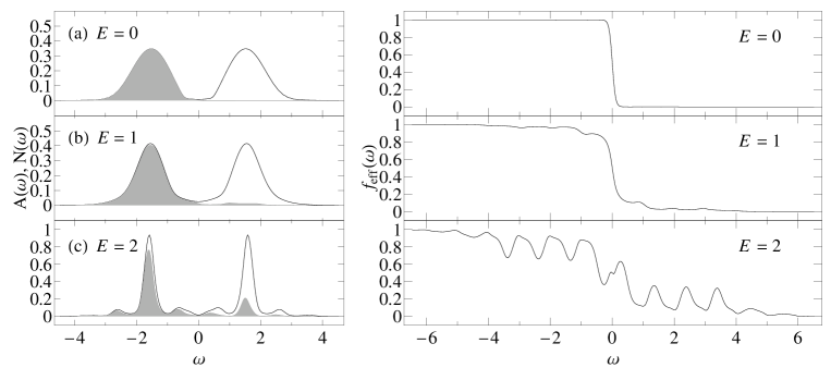
Figure 1: The local spectral function $A_{0}(\omega)$ (solid curves) and the particle number density $N_{0}(\omega)$ (shaded regions) (left panels), and the effective distribution function $f_{\rm eff}(\omega)$ (right) for $E=0$ (a), $E=1.0$ (b), $E=2.0$ (c) with $\Omega=1.0$, $U=3.0$, $\Gamma=0.05$ and $T=0.05$.

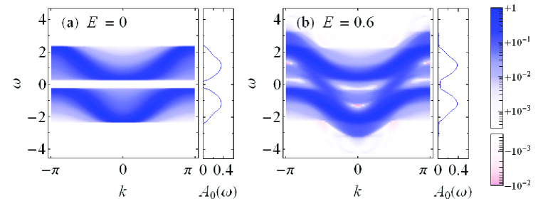
Figure 2: The gauge invariant spectral function $\tilde{A}_{0}({\boldsymbol{k}},\omega)$ (color-coded), and the local spectral function $A_{0}(\omega)$ (curves) for $E=0$ (a) and $E=0.6$ (b) with $\Omega=1.0$ and $U=2.2$ on the three dimensional cubic lattice, and ${\boldsymbol{k}}=k(1,1,1)$.

We consider the following quantities: the spectral function $A_{n}(\omega)=-\sum_{\boldsymbol{k}}{\rm Im}[(G_{\boldsymbol{k}}^{R})_{n}(\omega)]/\pi$ (Fig.1, left panels), the particle number density $N_{n}(\omega)=-i\sum_{\boldsymbol{k}}(G_{\boldsymbol{k}}^{<})_{n}(\omega)/2\pi$ (Fig.1), the effective distribution function $f_{\rm eff}(\omega)=N_{0}(\omega)/A_{0}(\omega)$ (Fig.1, right), the gauge invariant spectral function $\tilde{A}_{n}({\boldsymbol{k}},\omega)=-{\rm Im}[(\tilde{G}_{\boldsymbol{k}}^{R})_{n}(\omega)]/\pi$ (Fig.2), and the current $j(t)=ie\sum_{\boldsymbol{k}}\bar{\epsilon}_{{\boldsymbol{k}}-e{\boldsymbol{A}}(t)}G_{\boldsymbol{k}}^{<}(t,t)$ (Fig.3). Here $G^{R}$ and $G^{<}$ are the retarded and the lesser Green function respectively. Note that, to make the ${\boldsymbol{k}}$-dependent Green’s function gauge invariant, we use the modified function $\tilde{G}(t,{\boldsymbol{r}};t^{\prime},{\boldsymbol{r}}^{\prime})=\exp(ie\int_{(t,{\boldsymbol{r}})}^{(t^{\prime},{\boldsymbol{r}}^{\prime})}dx^{\nu}A_{\nu}(x))G(t,{\boldsymbol{r}};t^{\prime},{\boldsymbol{r}}^{\prime})$ [9].

4 Discussion

Figure 3: The current-voltage characteristic (solid curve) with $\Omega=1.0,U=3.0,\Gamma=0.05$, and $T=0.05$. We also show the linear-response result (dashed line) for comparison.

From the results one can see how the Mott insulating state is driven into a metallic state as one increases the intensity of the AC field beyond the linear-response regime. Specifically, we find in Fig.1 that the Mott gap collapses, and a new spectral weight emerges in the midgap region. Since the optical gap $\sim U(=3.0$ here) is greater than the frequency $\Omega(=1.0$ here), the direct interband transition is forbidden. However, if the intensity $E$ is sufficiently large, the electrons are excited to the conduction band through the midgap state, and the distribution function $f_{\rm eff}(\omega)$ (Fig.1) considerably deviates from the Fermi distribution $f(\omega)=1/(e^{\omega/T}+1)$ realized in equilibrium. More surprisingly, there is a region around certain $\omega$ where the population exceed those in lower-energy regions, a kind of population inversion. In the band dispersion of the system out of equilibrium shown in Fig.2, we again observe that the midgap state is induced by the field, whose band structure is roughly replicas of the original one with the spacing $\Omega$. Finally in Fig.3, the nonlinearity with the AC field is captured most clearly as the I-V characteristics obtained in the present method. Here $J\equiv{\rm Re}\;\frac{1}{\tau}\int_{0}^{\tau}dt\;e^{i\Omega t}j(t)$ is the current. When $E$ is small, the current is approximately proportional to $E$ as in the linear-response theory, but a nonlinear response becomes evident for $E\gtrsim 0.2$. This suggests that in the heart of the photoinduced insulator-metal transition lies the nonlinearity of the driving field.

During the preparation of this paper, we notice that a similar idea of using a matrix form was mentioned in ref. [10].

References

References

- [1] K. Miyano, T. Tanaka, Y. Tomioka, and Y. Tokura, Phys. Rev. Lett. 78, 4257 (1997).
- [2] M. Fiebig, K. Miyano, Y. Tomioka, and Y. Tokura, Science 280, 1925 (1998).
- [3] M. Matsubara, Y. Okimoto, T. Ogasawara, Y. Tomioka, H. Okamoto, and Y. Tokura, Phys. Rev. Lett. 90, 207401 (2007).
- [4] J. H. Shirley, Phys. Rev. 138, B979 (1965).
- [5] H. Sambe, Phys. Rev. A 7, 2203 (1973).
- [6] J. K. Freericks, V. M. Turkowski, and V. Zlatić, Phys. Rev. Lett. 97, 266408 (2006).
- [7] N. Tsuji, Master thesis, University of Tokyo, 2008.
- [8] N. Tsuji, T. Oka, and H. Aoki, in preparation.
- [9] D. G. Boulware, Phys. Rev. 151, 1024 (1966).
- [10] A. V. Joura, J. K. Freericks, and Th. Pruschke, cond-mat/0804.3077.