Photoproduction of $\pi^{+}\pi^{-}$ meson pairs on the proton

Abstract

The exclusive reaction $\gamma p\to p\pi^{+}\pi^{-}$ was studied in the photon energy range 3.0 - 3.8 GeV and momentum transfer range $0.4<-t<1.0$ GeV². Data were collected with the CLAS detector at the Thomas Jefferson National Accelerator Facility. In this kinematic range the integrated luminosity was about 20 pb^-1. The reaction was isolated by detecting the $\pi^{+}$ and proton in CLAS, and reconstructing the $\pi^{-}$ via the missing-mass technique. Moments of the di-pion decay angular distributions were derived from the experimental data. Differential cross sections for the $S$, $P$, and $D$-waves in the $M_{\pi^{+}\pi^{-}}$ mass range $0.4-1.4$ GeV were derived performing a partial wave expansion of the extracted moments. Besides the dominant contribution of the $\rho(770)$ meson in the $P$-wave, evidence for the $f_{0}(980)$ and the $f_{2}(1270)$ mesons was found in the $S$ and $D$-waves, respectively. The differential production cross sections $d\sigma/dt$ for individual waves in the mass range of the above-mentioned mesons were extracted. This is the first time the $f_{0}(980)$ has been measured in a photoproduction experiment.

I Introduction

The two pion channel offers the possibility of investigating various aspects of the meson resonance spectrum. It couples to the scalar-isoscalar channel that contains the $\sigma$, $f_{0}(980)$ and possibly a few more resonances with masses below $2\mbox{ GeV}$. It is the main decay mode of the lowest isoscalar-tensor $f_{2}(1270)$ resonance and it is the only decay mode of the isovector-vector resonance, the $\rho(770)$. Among all these, the $\rho$-meson is by far the most prominent and most extensively studied, both from the point of view of its production mechanisms and its internal properties. Nowadays the other resonances too are subjects of extensive theoretical and experimental investigation. The $\sigma$ meson is now established with pole mass and width determined with good accuracy Caprini:2005zr ; Kaminski:2006qe ; Kaminski:2006yv . However, its microscopic structure seems to be quite different from that of the $\rho$ and it is the subject of theoretical debate Pelaez:2003dy . The $f_{0}(980)$ is even a more enigmatic state: its experimental determination is complicated by its proximity to the $K{\bar{K}}$ threshold, and its QCD nature still awaits an explanation Bugg:2004xu . Finally, the $f_{2}(1270)$ has been represented so far as a Breit-Wigner resonance Kaminski:2006qe and appears to fit well into the quark model spectrum Godfrey:1985xj .

In this paper we focus on the scalar sector, using the $\rho$ meson as a benchmark for the analysis procedure. The $K{\bar{K}}$ channel from the same data set is currently being analyzed and in the near future a coupled-channels analysis will provide further constraints on the extraction of the meson properties.

For a long time most of our knowledge on the scalar meson spectrum was obtained from hadron-induced reactions, $\gamma\gamma$ collisions and studying the decays of various mesons, e.g. $\phi$, $J/\Psi$, $D$ and $B$. Very few studies were attempted with electromagnetic probes, in particular real photons, since their production cross sections are relatively small compared to the dominant production of vector mesons. On one hand, through vector meson dominance, the photon can be effectively described as a virtual vector meson. On the other hand, quark-hadron duality and the point-like-nature of the photon coupling make it possible to describe photo-hadron interactions at the QCD level. Recently, high-intensity and high-quality tagged-photon beams, as the one available at JLab, have opened a new window into this field.

In photoproduction processes, information about the $S$-wave strength can be extracted by performing a partial wave analysis. Angular distributions of photoproduced mesons and related observables, such as the moments of the angular distributions and the density matrix elements, are the most effective tools to look for interference patterns. An interference between the $S$-wave and the dominant $P$-wave was discovered in the moment analysis of $K^{+}K^{-}$ photoproduction on hydrogen, analyzing the data collected in the experiments performed at DESY Behrend and Daresbury Barber . In two-pion production experiments, such as reported in Refs. Ballam_1 ; Ballam_2 ; ABBHHM , moments and density matrix elements were used to analyze the properties of helicity amplitudes describing the photoproduction process. Unfortunately, only the dominant spin-1 partial wave of the $\pi^{+}\pi^{-}$ pair was taken into account. No attempt to obtain information about the $S$-wave amplitude was made. More recently, the HERMES experiment at DESY HERMES investigated the interference of the $P$-wave in the $\pi^{+}\pi^{-}$ system with the $S$ and $D$-waves in the $\pi^{+}\pi^{-}$ electroproduction process, and showed that such interference effects are measurable. The large photon virtuality $Q^{2}>$3 GeV² is, however, a crucial factor that distinguishes this analysis from the photoproduction analysis Ballam_1 ; Ballam_2 .

Theoretical models for $\pi^{+}\pi^{-}$ photoproduction have been investigated in a series of articles. A very successful approach is the one by Söding Soding and its numerous modifications Krass ; Kramer_Uretsky ; Pumplin ; Bauer . These models were able to describe the shift of the maximum of the $\pi^{+}\pi^{-}$ effective mass distribution with respect to the nominal $\rho$ mass and the asymmetric shape observed in SLAC Ballam_1 ; Ballam_2 and DESY ABBHHM ; Struczinski data. These properties are attributed to the interference of the dominating diffractive $\rho$ meson production, with its subsequent decay into $\pi^{+}\pi^{-}$, with the amplitudes corresponding to Drell-type diagrams in which the photon dissociates into $\pi^{+}$ and $\pi^{-}$, and one of the pions is elastically scattered off the proton. More recently, Gómez Tejedor and Oset GomezTejedor applied an effective Lagrangian to construct the photoproduction amplitudes. Their approach is limited to photon energies below 800 MeV and effective masses $M_{\pi\pi}$ smaller than 1 GeV. A two-stage approach for the $\pi^{+}\pi^{-}$ $S$-wave photoproduction was proposed in the model of Ref. Ji . First, a set of Born amplitudes, corresponding to photoproduction of $\pi^{+}\pi^{-}$, $\pi^{0}\pi^{0}$, $K^{+}K^{-}$ and $K^{0}{\bar{K}^{0}}$ pairs is calculated. Then the photoproduced meson pairs are subject to final-state interactions resulting in the $\pi^{+}\pi^{-}$ system KLM1994 ; KL1995 ; L1996 ; BLS . The coupled-channels calculations were separately performed for all isospin $I$ components of the transition matrix. Thus the $S$-wave amplitudes in that model account for the existence of the isoscalar $\sigma$, $f_{0}(980)$ and $f_{0}(1500)$, and the isovector $a_{0}(980)$ and $a_{0}(1450)$ resonances. The coupling of the $K\bar{K}$ isovector channel with the $\pi\eta$ amplitude is described in Ref. FL .

All theoretical approaches described above do not consider explicitly the $s$-channel production of baryon resonances contributing to the $p\pi\pi$ final state. Data from Refs. Ballam_1 ; ABBHHM ; Struczinski , as well as from more recent experimental studies ELSA , indicate that the contribution of baryon resonances, such as $\Delta^{++}$ and $\Delta^{0}$, dominate at lower incident photon energies (below 2 GeV). Furthermore, data obtained with the SAPHIR detector at ELSA for photon energies between 0.5 GeV and 2.6 GeV show that the contribution of baryonic resonances to the $\pi^{+}p$ and $\pi^{-}p$ mass distributions gradually decreases with photon energy.

In this paper we review the results of the analysis of $\pi^{+}\pi^{-}$ photoproduction in the photon energy range 3.0 - 3.8 GeV and momentum transfer squared $-t$ between 0.4 GeV² and 1 GeV², where the di-pion effective mass $M_{\pi\pi}$ varies from 0.4 GeV to 1.4 GeV. The main results were previously reported in Ref. PRL_f0 . We are not aware of any previous evidence of scalar mesons, in particular of the $f_{0}(980)$, in photoproduction of pion pairs. This effective mass region is dominated by the production of the $\rho(770)$ resonance in the $P$-wave. From other experiments, such as pion-nucleon collisions $\pi^{-}p\to\pi^{+}\pi^{-}n$ Grayer ; Becker or nucleon-antinucleon annihilation Amsler1 , there is some evidence that resonant states are formed in the $S$-wave. These resonances have been neglected in previous experimental analyses of $\pi^{+}\pi^{-}$ photoproduction and, to our knowledge, the current analysis is the first one that explicitly takes into account the possibility that the $S$-wave is produced in the $\pi^{+}\pi^{-}$ system.

In the following, some details are given on the experiment and data analysis (Sec. II), on the extraction of the angular moments of the di-pion system (Sec. III), and the fit of the moments using a dispersion relation (Sec. IV). Results of the partial wave analysis (differential cross section for each partial wave and the spin density matrix elements) and the physics interpretation are reported in Sec. V.

II Experimental procedures and data analysis

II.1 The photon beam and the target

The measurement was performed using the CLAS detector B00 in Hall B at Jefferson Lab with a bremsstrahlung photon beam produced by a continuous 60-nA electron beam of energy $E_{0}$ = 4.02 GeV impinging on a gold foil of thickness $8\times 10^{-5}$ radiation lengths. A bremsstrahlung tagging system SO99 with a photon energy resolution of 0.1$\%$ $E_{0}$ was used to tag photons in the energy range from 1.6 GeV to a maximum energy of 3.8 GeV. In this analysis only the high-energy part of the photon spectrum, ranging from 3.0 to 3.8 GeV, was used. $e^{+}$ $e^{-}$ pairs produced by the interaction of the photon beam on a thin gold foil were used to continuously monitor the photon flux during the experiment. Absolute normalization was obtained by comparing the $e^{+}$ $e^{-}$ pair rate with the photon flux measured by a total absorption lead-glass counter in dedicated low-intensity runs. The energy calibration of the Hall-B tagger system was performed both by a direct measurement of the $e^{+}e^{-}$ pairs produced by the incoming photons tag-abs_cal and by applying an over-constrained kinematic fit to the reaction $\gamma p\to p\pi^{+}\pi^{-}$, where all particles in the final state were detected in CLAS tag-kinefit . The quality of the calibrations was checked by looking at the mass of known particles, as well as their dependence on other kinematic variables (photon energy, detected particle momenta and angles).

The target cell, a Mylar cylinder 4 cm in diameter and 40-cm long, was filled by liquid hydrogen at 20.4 K. The luminosity was obtained as the product of the target density, target length and the incoming photon flux corrected for data-acquisition dead time. The overall systematic uncertainty on the run luminosity was estimated to be in the range of 10$\%$, dominated by the uncertainties on the photon flux.

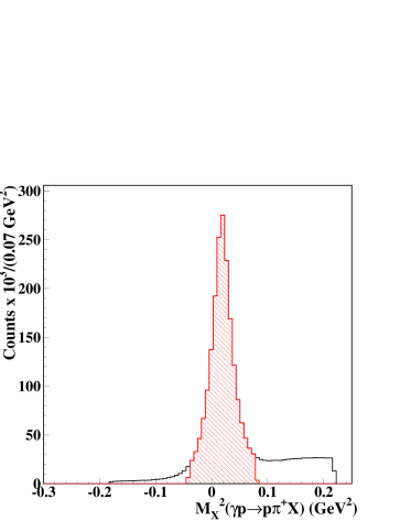
Figure 1: Missing mass squared for the reaction $\gamma p\to p\pi^{+}X$ and the $\pi^{-}$ peak. The shaded area indicates the retained events.

II.2 The CLAS detector

Outgoing hadrons were detected in the CLAS spectrometer. Momentum information for charged particles was obtained via tracking through three regions of multi-wire drift chambers DC within a toroidal magnetic field ($\sim 0.5$ T) generated by six superconducting coils. The polarity of the field was set to bend the positive particles away from the beam line into the acceptance of the detector. Time-of-flight scintillators (TOF) were used for charged hadron identification Sm99 . The interaction time between the incoming photon and the target was measured by the start counter (ST) ST . This is made of 24 strips of 2.2-mm thick plastic scintillator surrounding the hydrogen cell with a single-ended PMT-based read-out. A time resolution of $\sim$300 ps was achieved.

The CLAS momentum resolution, $\sigma_{p}/p$, ranges from 0.5 to 1%, depending on the kinematics. The detector geometrical acceptance for each positive particle in the relevant kinematic region is about 40%. It is somewhat less for low-energy negative hadrons, which can be lost at forward angles because their paths are bent toward the beam line and out of the acceptance by the toroidal field. Coincidences between the photon tagger and the CLAS detector triggered the recording of the events. The trigger in CLAS required a coincidence between the TOF and the ST in at least two sectors, in order to select reactions with at least two charged particles in the final state. An integrated luminosity of 70 pb^-1 ($\sim 20$ pb^-1 in the range 3.0$<E_{\gamma}<$3.8 GeV) was accumulated in 50 days of running in 2004.

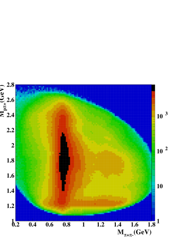
Figure 2: Two dimensional plot of the invariant masses obtained combining pairs of particles of the exclusive reaction $\gamma p\to p\pi^{+}\pi^{-}$.

Figure 3: Invariant masses obtained combining pairs of particles of the exclusive reaction $\gamma p\to p\pi^{+}\pi^{-}$. Upper panel $M_{\pi^{+}\pi^{-}}$; lower panel left $M_{p\pi^{+}}$; lower panel right $M_{p\pi^{-}}$. Spectra are not corrected for the detector acceptance.

II.3 Data analysis and reaction identification

The raw data were passed through the standard CLAS reconstruction software to determine the four-momenta of detected particles. In this phase of the analysis, corrections were applied to account for the energy loss of charged particles in the target and surrounding materials, misalignments of the drift chamber’s positions, and uncertainties in the value of the toroidal magnetic field.

The reaction $\gamma p\to p\pi^{+}\pi^{-}$ was isolated detecting the proton and the $\pi^{+}$ in the CLAS spectrometer, while the $\pi^{-}$ was reconstructed from the four-momenta of the detected particles by using the missing-mass technique. In this way the exclusivity of the reaction is ensured, keeping the contamination from the multi-pion background to a minimum. Figure 1 shows the $\pi^{-}$ missing mass squared. The background below the missing pion peak appears as a smooth contribution in the $\pi\pi$ invariant mass without creating narrow structures.

To avoid edge regions in the detector acceptance, only events within a fiducial volume were retained in this analysis. In the laboratory reference system, cuts were defined for the minimum hadron momentum ($p_{proton}>0.32$ GeV and $p_{\pi^{+}}>0.125$ GeV), and the minimum and maximum azimuthal angles ($\theta_{proton,\pi^{+}}>10^{\circ}$ and $\theta_{\pi^{+}}<120^{\circ}$). The fiducial cuts were defined comparing in detail the experimental data distributions with the results of the detector simulation. The minimum momentum cuts were tuned for different hadrons to take into account the energy loss by ionization of the particles.

After all cuts, 41M events were identified as produced in the exclusive reaction $\gamma p\to p\pi^{+}\pi^{-}$. The other event topologies, with at least two hadrons in the final state ($p\pi^{-}$, $\pi^{+}\pi^{-}$, $p\pi^{+}\pi^{-}$), were not used since in the kinematics of interest for this analysis ($-t<1$ GeV²), the collected data are about one order of magnitude less due to the detector acceptance. Figures  2 and  3 show the invariant mass spectra of the different combinations of particles in the final state. The $\rho(770)$ dominates the $\pi\pi$ spectrum and the $\Delta(1232)^{++}$ peak is clearly visible in the $p\pi^{+}$ invariant mass. Figure 2 shows a small overlap between the $\Delta(1232)^{++}$ and the $\pi\pi$ spectrum. Baryonic resonances in the $p\pi^{-}$ invariant mass spectrum are less pronounced. It has to be noted that the projection of the baryon resonance peaks in the $\pi\pi$ spectrum results in a smooth contribution and cannot create narrow structures. The effect of this background was extensively studied as discussed in Sec.V.3.

III Moments of the di-pion angular distribution

In this section we consider the analysis of moments of the di-pion angular distribution defined as:

$$\langle Y_{LM}\rangle(E_{\gamma},t,M_{\pi\pi})=\sqrt{4\pi}\int d\Omega_{\pi}{{d\sigma}\over{dtdM_{\pi\pi}d\Omega_{\pi}}}Y_{LM}(\Omega_{\pi}),$$ (1)

where $d\sigma$ is the differential cross section (in momentum transfer $t$ and di-pion invariant mass $M_{\pi\pi}$), $Y_{LM}$ are spherical harmonic functions of degree $L$ and order $M$, and $\Omega_{\pi}=(\theta_{\pi},\phi_{\pi})$ are the polar and azimuthal angles of the $\pi^{+}$ flight direction in the $\pi^{+}\pi^{-}$ helicity rest frame. For the definition of the angles in the di-pion system we follow the convention of Ref. Ballam_1 . It follows from Eq. 1 that, for a given $E_{\gamma},t$ and di-pion mass $M_{\pi\pi}$, $\langle Y_{00}\rangle$ corresponds to the di-pion production differential cross section $d\sigma/dtdM_{\pi\pi}$.

There are many advantages in defining and analyzing moments rather than proceeding via a direct partial wave fit of the angular distributions. Moments can be expressed as bi-linear in terms of the partial waves and, depending on the particular combination of $L$ and $M$, show specific sensitivity to a particular subset of them. In addition, they can be directly and unambiguously derived from the data, allowing for a quantitative comparison to the same observables calculated in specific theoretical models.

Extraction of moments requires that the measured angular distribution is corrected by the detector acceptance. We studied three methods for implementing acceptance corrections. In the first two methods, the moments were expanded in a model-independent way in a set of basis functions and, after weighting with Monte Carlo events, they were compared to the data by maximizing a likelihood function. The first of these two parametrizes the theory in terms of simplified $amplitudes$, while the second uses directly $moments$ as defined above. The approximations in these methods have to do with the choice of the basis and depend on the number of basis functions used. The systematic effect of such truncations was studied and the main results are reported below. In the last method, data and Monte Carlo were binned in all kinematical variables. The data were then corrected by the acceptance defined as the ratio of reconstructed over generated Monte Carlo events in that bin. Since it was found to be not reliable in bins where the acceptance was small or vanishing, this method was only used as a check of the others and was not included in the final determination of the experimental moments.

III.1 Detector efficiency

The CLAS detection efficiency for the reaction $\gamma p\to p\pi^{+}\pi^{-}$ was obtained by means of detailed Monte Carlo studies, which included knowledge of the full detector geometry and a realistic response to traversing particles. Events were generated according to three-particle phase space with a bremsstrahlung photon energy spectrum. A total of $4$ billion events were generated in the energy range 3.0 GeV $<E_{\gamma}<$ 3.8 GeV and covered the allowed kinematic range in $-t$ and $M_{\pi\pi}$. About 700M events were reconstructed in the $M_{\pi\pi}$ and $-t$ ranges of interest (0.4 GeV $<M_{\pi\pi}<$ 1.4 GeV , 0.1 GeV${}^{2}<-t<$ 1.0 GeV²). This corresponds to more than fifteen times the statistics collected in the experiment, thereby introducing a negligible statistical uncertainty with respect to the statistical uncertainty of the data.

III.2 Extraction of the moments via likelihood fit of experimental data

Moments were derived from the data using detector efficiency-corrected fitting functions. As mentioned above, the expected theoretical yield was parametrized in terms of appropriate physics functions: production amplitudes in one case and moments of the cross section in the other. The theoretical expectation, after correction for acceptance, was compared to the experimental yield. Parameters were extracted by maximizing a likelihood function defined as:

$${\cal L}\sim\Pi_{a=1}^{n}\left[{\eta(\tau_{a}){I(\tau_{a})}\over{\int d\tau\eta(\tau)I(\tau)}}\right].$$ (2)

Here $a$ represents a data event, $n=\Delta N$ is the number of data events in a given $(E_{\gamma},-t,M_{\pi\pi})$ bin (i.e. the fit is done independently in each bin), $\tau_{a}$ represents the set of kinematical variables of the $a^{th}$ event, $\eta(\tau_{a})$ is the corresponding acceptance derived by Monte Carlo simulations and $I(\tau_{a})$ is the theoretical function representing the expected event distribution. The measure $d\tau$ includes the phase space factor and the likelihood function is normalized to the expected number of events in the bin

$${\bar{n}}=\int d\tau\eta(\tau)I(\tau).$$ (3)

The advantage of this approach lies in avoiding binning the data and the large uncertainties related to the corrections in regions of CLAS with vanishing efficiencies. Comparison of the results of the two different parametrizations allows one to estimate the systematic uncertainty related to the procedure. In the following, we describe the two approaches in more detail.

III.2.1 Parametrization with amplitudes

The expected theoretical yield in each bin is described as:

$$I(\tau_{a})=4\pi\left|\sum_{L=0}^{L_{max}}\sum_{M=-L}^{L}a_{LM}(E_{\gamma},-t,M_{\pi\pi})Y_{LM}(\Omega_{\pi})\right|^{2}.$$ (4)

This parametrization has the benefit that the intensity function $I(\tau_{a})$ is by construction positive. However, it can lead to ambiguous results since it has more parameters than can be determined from the data. In addition, for practical reasons, the parametrization involves a cutoff, $L_{max}$, in the maximum number of amplitudes. For a specific choice of $L_{max}$, the number of fit parameters is given by $2(L_{max}+1)^{2}$. We also note that these amplitudes are not the same as the partial wave amplitudes in the usual sense of a di-pion photoproduction amplitude, since the latter depends on the nucleon and photon spins.

After removing the irrelevant constants, the fit is performed minimizing the function:

$$-\ln{\cal L} = -\sum_{a=1}^{\Delta N}\ln\eta(\tau_{a})I(\tau_{a})$$

$$+ \Delta N\ln\sum_{L^{\prime}M^{\prime};LM}{\tilde{a}}^{*}_{L^{\prime}M^{\prime}}{\tilde{a}}_{LM}\Psi_{L^{\prime}M^{\prime};L,M},$$

where we have introduced the rescaled amplitudes ${\tilde{a}}_{LM}(E_{\gamma},-t,M_{\pi\pi})$ defined by:

$${\tilde{a}}_{LM}=\sqrt{{\eta}}a_{LM},$$ (6)

and the acceptance matrix $\Psi(E_{\gamma},-t,M_{\pi\pi})$ was computed using Monte Carlo events as:

$$\eta\Psi_{L^{\prime}M^{\prime};LM}={{4\pi}\over{\Delta N_{Gen}}}\sum_{a=1}^{\Delta N_{Rec}}Y^{*}_{L^{\prime}M^{\prime}}(\Omega_{\pi})Y_{LM}(\Omega_{\pi}),$$ (7)

where $\Delta N_{Gen}$ and $\Delta N_{Rec}$ are the number of generated and reconstructed events, respectively.

Fits were done using MINUIT with the analytical expression for the gradient, and using the SIMPLEX procedure followed by MIGRAD minuit . After each fit, the covariance matrix was checked and if it was not positive definite, the fit was restarted with random input parameters. At the end, the uncertainties were computed from the full covariance matrix.

III.2.2 Parametrization with moments

The expected theoretical yield in each $(E_{\gamma},-t,M_{\pi\pi})$ bin is described as:

$$I(\tau_{a})=\sqrt{4\pi}\sum_{L=0}^{L_{max}}\sum_{M=0}^{L}\langle\tilde{Y}_{LM}\rangle\mbox{ Re}Y_{LM}(\Omega_{\pi}).$$ (8)

The parametrization in terms of the moments directly gives the quantities we are interested in (moments $\langle\tilde{Y}_{LM}\rangle$). However, the fit has to be restricted to make sure the intensity is positive. As in the amplitude parametrization, a cutoff $L_{max}$ in the maximum number of moments has to be used. The number of fit parameters is given by $(L_{max}+1)(L_{max}+2)/2$. As $L_{max}$ increases, moments with $L$ close to $L_{max}$ show a significant variation, while moments with the lowest $L$ remain unchanged.

The expected (acceptance-corrected) distribution is then given by:

$$I(\tau_{a})=\sqrt{4\pi}\sum_{L,M}\left[\eta_{LM}\mbox{ Re}Y_{LM}(\Omega_{\pi})\right]\langle\tilde{Y}_{LM}\rangle.$$ (9)

The function to be minimized with respect to $\langle\tilde{Y}_{LM}\rangle$ ($L>0$) is then given by:

$$-2\ln{\cal L}=-2\sum_{a=1}^{\Delta N}\ln I(\tau_{a}),$$ (10)

with the coefficients $\eta_{LM}(E_{\gamma},-t,M_{\pi\pi})$ computed using Monte Carlo events

$$\eta_{LM}={{\sqrt{4\pi}}\over{\Delta N_{Gen}}}\sum_{i}^{\Delta N_{Rec}}{{\mbox{ Re}Y_{LM}(\Omega_{i})}\over{\epsilon_{L}}},$$ (11)

where $\epsilon_{L}=1$ for $L=0$ and $1/2$ for all other $(LM)$. For $L_{max}\leq 4$, the results are similar to what was obtained with the previous method, showing the same stability against $L_{max}$ truncation and a similar goodness of the fit. To check the sensitivity of the likelihood fit to the parameter initialization, moments were extracted in three different ways: 1) using random initialization for all parameters; 2) fixing the parameters up to $L=2$ to the ones obtained from a fit with $L_{max}=2$, and randomly initializing the others; 3) starting with parameters obtained in 2) and then releasing all parameters. The three different methods gave consistent results and the difference of moments obtained using the different procedures was used to evaluate the systematic uncertainty related to the fit procedure.

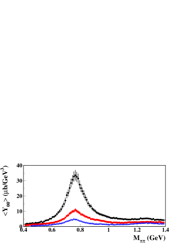
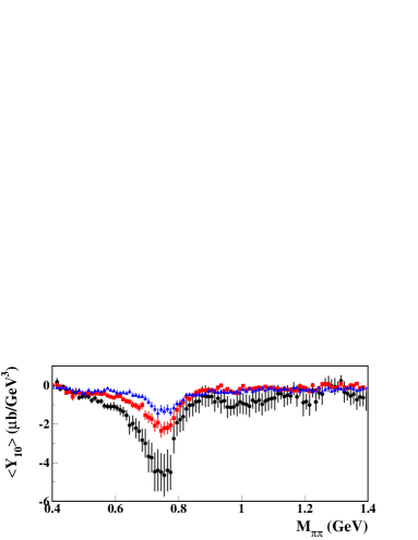
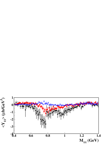
Figure 4: Moments of the di-pion angular distribution in $3.2<E_{\gamma}<3.4$ GeV and $-t=0.45\pm 0.05$ GeV² (black), $-t=0.65\pm 0.05$ GeV² (red) and $-t=0.95\pm 0.05$ GeV² (blue). Error bars include both statistical and systematic uncertainties as explained in the text.

III.2.3 Methods comparison and final results

Moments derived by the different procedures agreed qualitatively. The most stable results were obtained by using the first parametrization, although we do find occasionally large bin-to-bin fluctuations. However, there are no a priori reasons to prefer one of the two methods and we consider the discrepancies between the fit results as a good estimate of the systematic uncertainty associated with the moments extraction. The final results are given as the average of the first method (parametrization with amplitudes) and the second method (parametrization with moments) with the three fit initializations:

$$Y_{final}={{1}\over{4}}\sum_{i=1,4\,Methods}{Y_{i}},$$ (12)

where $Y$ stands for $\langle Y_{LM}\rangle(E_{\gamma},t,M_{\pi\pi})$.

The total uncertainty on the final moments was evaluated adding in quadrature the statistical uncertainty, $\delta Y_{MINUIT}$ as given by MINUIT, and two systematic uncertainty contributions: $\delta Y_{syst\,\,fit}$ related to the moment extraction procedure, and $\delta Y_{syst\,\,norm}$, the systematic uncertainty associated with the photon flux normalization (see Sec. II).

$$\delta Y_{final}=\sqrt{\delta Y_{MINUIT}^{2}+\delta Y_{syst\,\,fit}^{2}+\delta Y_{syst\,\,norm}^{2}}$$ (13)

with:

$$\delta Y_{syst\,\,fit} = \sqrt{\sum_{i=1,4\,Methods}{({Y_{i}}-Y_{final})^{2}\over{4-1}}}$$ (14)

$$\delta Y_{syst\,\,norm} = 10\%\cdot Y_{final}.$$ (15)

For most of the data points, the systematic uncertainties dominate over the statistical uncertainty. Samples of the final experimental moments are shown in Figs. 4, 5, 6, and 7. The whole set of moments resulting from this analysis is available at the Jefferson Lab jlab-db and the Durham dhuram-db databases.

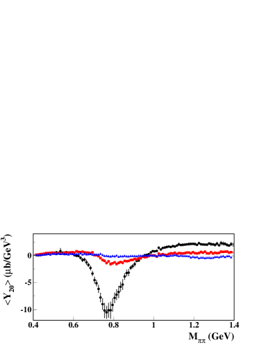
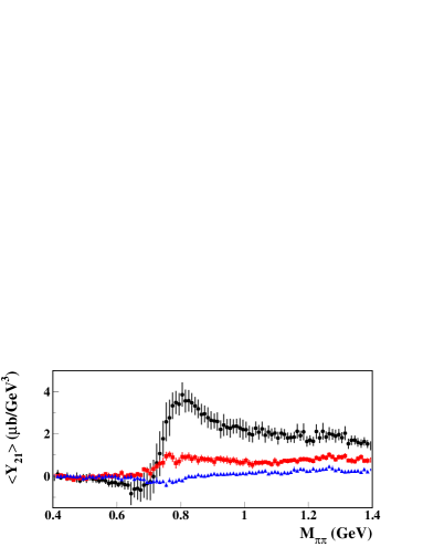
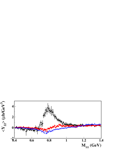
Figure 5: Moments of the di-pion angular distribution in $3.2<E_{\gamma}<3.4$ GeV and $-t=0.45\pm 0.05$ GeV² (black), $-t=0.65\pm 0.05$ GeV² (red) and $-t=0.95\pm 0.05$ GeV² (blue). Error bars include both statistical and systematic uncertainties as explained in the text.

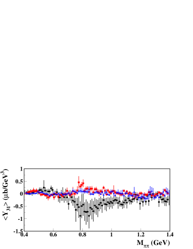
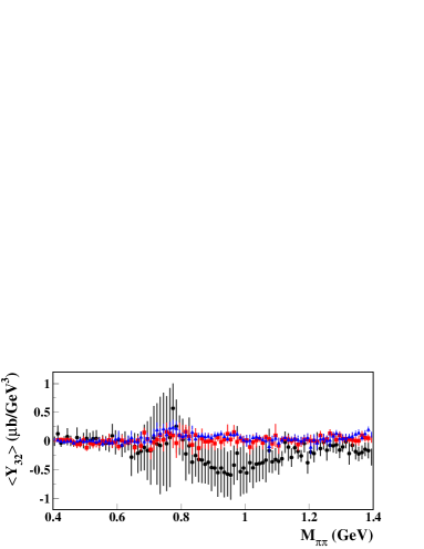
Figure 6: Moments of the di-pion angular distribution in $3.2<E_{\gamma}<3.4$ GeV and $-t=0.45\pm 0.05$ GeV² (black), $-t=0.65\pm 0.05$ GeV² (red) and $-t=0.95\pm 0.05$ GeV² (blue). Error bars include both statistical and systematic uncertainties as explained in the text.

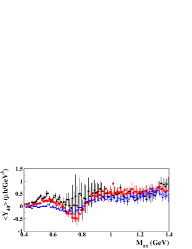
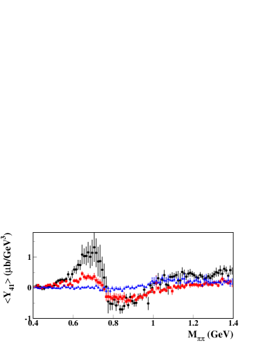
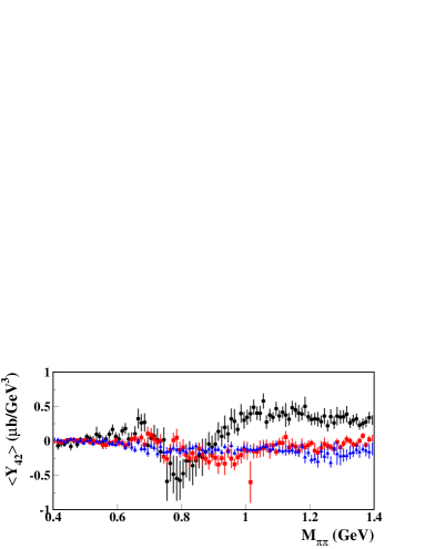
Figure 7: Moments of the di-pion angular distribution in $3.2<E_{\gamma}<3.4$ GeV and $-t=0.45\pm 0.05$ GeV² (black), $-t=0.65\pm 0.05$ GeV² (red) and $-t=0.95\pm 0.05$ GeV² (blue). Error bars include both statistical and systematic uncertainties as explained in the text.

As a check of the whole procedure, the differential cross section $d\sigma/dt$ for the $\gamma p\to p\rho(770)$ meson has been extracted by fitting the $\langle Y_{00}\rangle$ moment in each $-t$ bin with a Breit-Wigner plus a first-order polynomial background. The agreement within the quoted uncertainties with a previous CLAS measurement Battaglieri , as well as the world data ABBHHM , gives us confidence in the analysis procedure.

IV Partial wave analysis

In the previous section we discussed how moments of the angular distribution of the $\pi^{+}\pi^{-}$ system, $\langle Y_{LM}\rangle$, were extracted from the data in each bin in photon energy, momentum transfer and di-pion mass. In this section we describe how partial waves were parametrized and extracted by fitting the experimental moments.

Moments can be expressed as bi-linear in terms of the amplitudes $a_{lm}=a_{lm}(\lambda,\lambda^{\prime},\lambda_{\gamma},E_{\gamma},t,M_{\pi\pi})$ with angular momentum $l$ and $z$-projection $m$ (in the chosen reference system $m$ coincides with the helicity of the di-pion system) as:

$$\langle Y_{LM}\rangle=\sum_{l^{\prime}m^{\prime},lm,\lambda,\lambda^{\prime}}C(l^{\prime}m^{\prime},lm,LM)\times a_{lm}\;a^{*}_{l^{\prime}m^{\prime}},$$ (16)

where $C$ are Wigner’s 3jm coefficients, $\lambda_{\gamma}$ is the helicity of the photon, and $\lambda$ and $\lambda^{\prime}$ are the initial and final nucleon helicity, respectively. The explicit forms of the moments with $L\leq 4$ in terms of amplitudes with $l=0$ ($S$-wave), $l=1$ ($P$-wave), $l=2$ ($D$-wave), and $l=3$ ($F$-wave) are given in Appendix A.

IV.1 Helicities, isospin and coupled-channels dependence

The photon helicity was restricted to $\lambda_{\gamma}=+1$ since the other amplitudes are related by parity conservation. In addition, some approximations in the parametrization of the partial waves were adopted to reduce the number of free parameters in the fit and are discussed below.

• The number of waves was reduced restricting the analysis to $|m|\leq 1$ since $m=2$ is only possible for $l\geq 2$ ($D$ and $F$ waves), which are expected to be small in the mass range considered Ballam_1 ; Ballam_2 . In the chosen reference system, $m$ coincides with the helicity of the di-pion system and, since we used as a reference the wave with $\lambda_{\gamma}=+1$, the three values of $m$ have a simple interpretation in terms of helicity transfer from the photon to the $\pi\pi$-system: $m=+1$ corresponds to the non-helicity-flip amplitude ($s$-channel helicity conserving) that is expected to be dominant Ballam_2 , while $m=0,-1$ correspond to one and two units of helicity flip, respectively. In the case of the $S$-wave ($l=m=0$), only one amplitude is considered.

• The dependence on the nucleon helicity was simplified as follows. For a given $l,m,E_{\gamma},t$ set, there are four independent partial wave amplitudes corresponding to the four combinations of initial and final nucleon helicity, $\lambda$ and $\lambda^{\prime}$. It is expected that the dominant amplitudes require no nucleon helicity flip Ballam_2 . Without nucleon polarization information it is not possible to extract all four amplitudes. Thus our strategy is to consider in the analysis only the dominant ones or to exploit possible relations among them. For example, in the Regge $\rho$ and $\omega$ exchange model, the following relations are satisfied by the $S$-wave amplitudes: $(\lambda\lambda^{\prime})=(++)=(--)$ and $(+-)=-(-+)$, where $\pm$ corresponds to helicity $\pm 1/2$. More generally, by examining the experimental moments, we observe that the interference between the dominant $P$-wave, seen in the $\langle Y_{21}\rangle$ moment in the $\rho$ region, indicates that the $P_{m=+1}$ and the $P_{m=0}$ amplitudes are out of phase. For a single nucleon-helicity amplitude, this would imply a difference between the $\langle Y_{11}\rangle$ and $\langle Y_{10}\rangle$ moments, arising primarily from the interference between the $S$-wave and the $P_{m=+1}$ and $P_{m=0}$ waves, respectively, in the $\rho$ region where the $S$ amplitude does not vary substantially. The data suggests, however, that both $\langle Y_{11}\rangle$ and $\langle Y_{10}\rangle$ peak near the position of the $\rho$. A possible explanation for the behavior of the data is the following: the dominant $P_{m=+1}$ amplitude may originate from the helicity-non-flip diffractive process and the $P_{m=0}$ amplitude from a nucleon-helicity-flip vector exchange, which is also expected to contribute to the $S$-wave production. This would also explain why the $\langle Y_{11}\rangle$ and $\langle Y_{10}\rangle$ moments have comparable magnitudes. To accommodate such behavior, at least two nucleon-helicity amplitudes are required. In addition, since strong interactions conserve isospin, it is convenient to write the $\pi\pi$ amplitudes in the isospin basis. Each amplitude was then expressed as a linear combination of $\pi\pi$ amplitudes of fixed isospin $I$ (with $I=0,1,2$).

• The coupling of the $\pi\pi$ system to other channels was taken into account introducing a multi-dimension channel space: for a given isospin $I$ in the partial wave $l$, the amplitudes depend also on an index $\alpha$ that runs over different di-meson systems. For example, $\alpha=1$ corresponds to $\pi\pi$, $\alpha=2$ to $K{\bar{K}}$, $\alpha=3$ to $\eta\eta$, etc. In the subsequent analysis we will restrict the channel space to include the $\pi\pi$ and $K{\bar{K}}$ channels, which are the only channels relevant in the energy range considered.

  According to these considerations, the moments were fitted to a set of amplitudes given by:

  $$a^{I,\alpha}_{lm,i}(E_{\gamma},t,M_{\pi\pi})$$ (17)

  for each $l,m$, $|m|\leq 1$, with $i=1,2$ corresponding to the nucleon helicity non-flip and helicity-flip of one unit, isospin $I=0,1,2$ and channel $\alpha$.

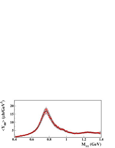
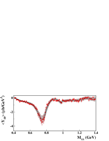
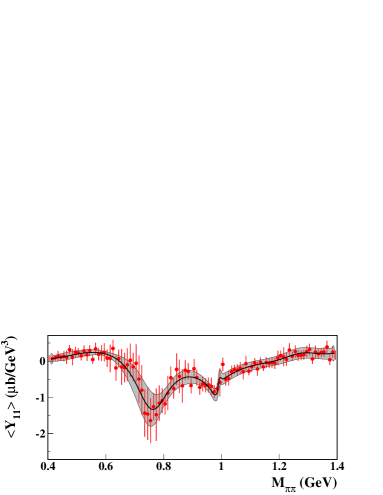
Figure 8: Fit result (black line) of the final experimental moments (in red) for $3.2<E_{\gamma}<3.4$ GeV and $0.5<-t<0.6$ GeV². The systematic uncertainty and fit uncertainty are added in quadrature and are shown by the gray band.

IV.2 Amplitude parametrization

For each helicity state of the target $\lambda$, recoil nucleon $\lambda^{\prime}$, and $\pi\pi$ system $m$, in a given $E_{\gamma}$ and $t$ bin, the corresponding helicity amplitude $a_{lm}(s=M^{2}_{\pi\pi})$, was expressed using a dispersion relation Aitchison:1976nk ; aitchison-1 ; aitchison-2 ; ascoli ; goradia ; Bowler:1975my ; Basdevant:1976jg as follows:

$$a_{lm,I}(s) = {1\over 2}[I+S_{lm,I}(s)]\tilde{a}_{lm,I}(s)$$

$$- {1\over{\pi}}D_{lm,I}^{-1}(s)PV\int_{s_{th}}ds^{\prime}{{N_{lm,I}(s^{\prime})\rho(s^{\prime})\tilde{a}_{lm,I}(s^{\prime})}\over{s^{\prime}-s}},$$

where $PV$ represents the principal value of the integral and $\rho$ corresponds to the phase space term. In this expression, $I$ and $S_{lm,I}$ are matrices in the multi-channel space ($\pi\pi$, $KK$), as mentioned above. $N_{lm,I}$ and $D_{lm,I}$ can be written in terms of the scattering matrix of $\pi\pi$ scattering, chosen to reproduce the known phase shifts, inelasticities Oller:1998hw ; Oller:1998zr , and the isoscalar ($l=S,D$), isovector ($l=P,F$) and isotensor ($l=S,D$) amplitudes in the range $0.4\mbox{ GeV}<\sqrt{s}<1.4\mbox{ GeV}$. Finally, the amplitude $\tilde{a}_{lm,I}$ represents our ignorance about the production process.

As a function of $s=M^{2}_{\pi\pi}$, $a_{lm,I}$ have cuts for $s>4m_{\pi}^{2}$ (right-hand cut) and for $s<m_{\pi}^{2}$ (left-hand cut). The left-hand cut reflects the nature of particle exchanges determining the $\pi\pi$ photoproduction amplitude, while the right-hand cut accounts for the final-state interactions of the produced pions. In Eq. IV.2, these discontinuities are taken into account by the functions $N_{lm,I}$ and $D_{lm,I}$, while $\tilde{a}_{lm,I}(s)$ does not have singularities for $s>4m_{\pi}^{2}$ and can be expanded in a Taylor series:

$$\tilde{a}_{lm,I}=\left[{\cal A}+{\cal B}s+{\cal C}s^{2}+\cdots\right][k]$$ (19)

with ${\cal A},{\cal B},\dots$ being matrices of numerical coefficients to be determined by the simultaneous fit of the angular moments defined in Eq. 16 and $[k]=k_{\alpha}^{l}\delta_{\alpha,\beta}$ used to take into account the threshold behavior in the $l$-th partial wave. All amplitudes but the scalar-isoscalar are saturated by the $\pi\pi$ state. For the scalar-isoscalar amplitude, the $K\bar{K}$ channel was also included. In addition, to reduce sensitivity to the large energy behavior of the ($\pi\pi$,$K\bar{K}$) amplitudes, the real part of the integral was subtracted and replaced by a polynomial in $s$, whose coefficients were also fitted.

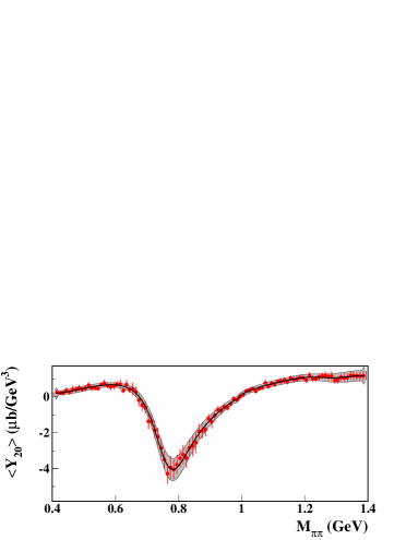
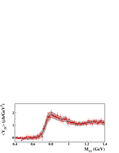
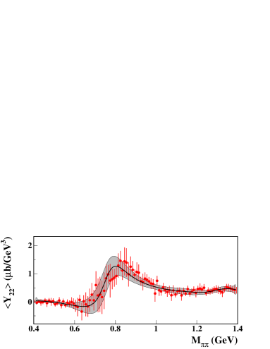
Figure 9: Fit result (black line) of the final experimental moments (in red) for $3.2<E_{\gamma}<3.4$ GeV and $0.5<-t<0.6$ GeV². The systematic uncertainty and fit uncertainty are added in quadrature and are shown by the gray band.

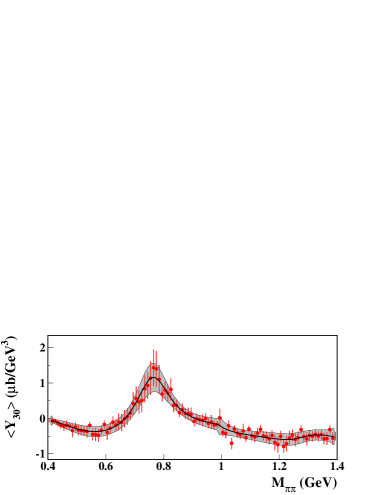
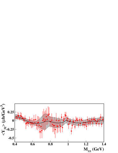
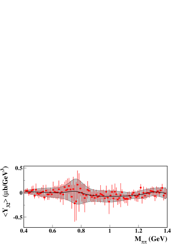
Figure 10: Fit result (black line) of the final experimental moments (in red) for $3.2<E_{\gamma}<3.4$ GeV and $0.5<-t<0.6$ GeV². The systematic uncertainty and fit uncertainty are added in quadrature and are shown by the gray band.

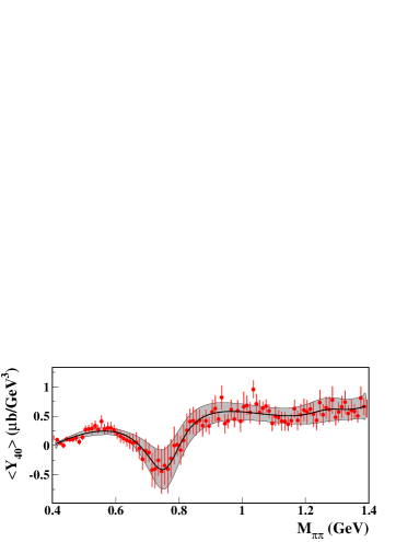
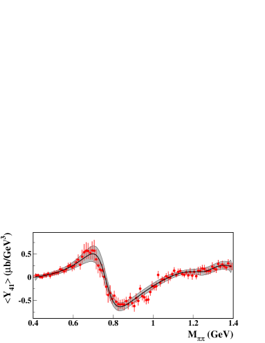
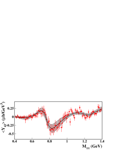
Figure 11: Fit result (black line) of the final experimental moments (in red) for $3.2<E_{\gamma}<3.4$ GeV and $0.5<-t<0.6$ GeV². The systematic uncertainty and fit uncertainty are added in quadrature and are shown by the gray band.

V Results

V.1 Fit of the moments

Using the parametrization of the partial waves described in the previous section, we fitted all moments $\langle Y_{LM}\rangle$ with $L\leq 4$ and $M\leq 2$ using amplitudes with $l\leq 3$ (up to $F$-waves). In Figs. 8, 9, 10, and 11 we present a sample of the fit results for $E_{\gamma}=3.3\pm 0.1$ GeV and $0.5<|t|<0.6$ GeV².

To properly take into account the statistical and systematic uncertainty contributions to the experimental moments described in Sec. III, the four sets of moments resulting from the different fit procedures were individually fitted and the results were averaged, obtaining the central value shown by the black line in the figures. The error band, shown as a gray area, was calculated following the same procedure adopted for the experimental moments. The final uncertainty was computed as the sum in quadrature of the statistical uncertainty of the fit and the two systematic uncertainty contributions. The first is related to the moment extraction procedure and is evaluated as the variance of the four fit results. The latter is associated with the photon flux normalization and is estimated to be 10%. The central values and uncertainties for all the observables of interest discussed in the following sections were derived from the fit results with the same procedure.

The moment $\langle Y_{00}\rangle$, corresponding to the differential production cross section $d\sigma/dtdM$, shows the dominant $\rho(770)$ meson peak. In the $\langle Y_{10}\rangle$ and $\langle Y_{11}\rangle$ moments, the contribution of the $S$-wave is maximum and enters via interference with the $P$-wave. In particular the structure at $M_{\pi\pi}\sim 0.77\mbox{ GeV}$ in $\langle Y_{11}\rangle$ is due to the interference of the $S$-wave with the dominant, helicity-non-flip wave, $P_{m=+1}$. In the $\langle Y_{10}\rangle$ moment the same structure is due to the interference with the $P_{m=0}$ wave, which corresponds to one unit of helicity flip. A second dip near $M_{\pi\pi}=1\mbox{ GeV}$ is clearly visible and corresponds to the production of a resonance that we interpret as the $f_{0}(980)$.

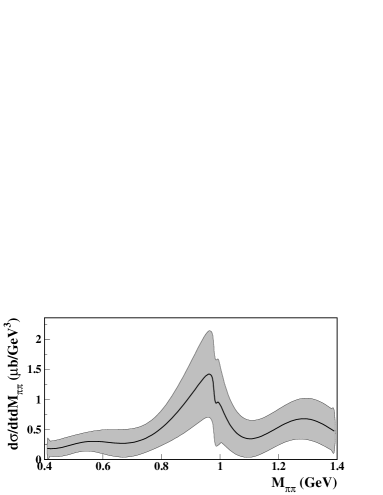
Figure 12: $S$-wave cross section derived by the fit in the $3.2<E_{\gamma}<3.4$ GeV and $0.5<-t<0.6$ GeV² bin. The systematic and the fit uncertainties are added in quadrature and are shown by the gray band.

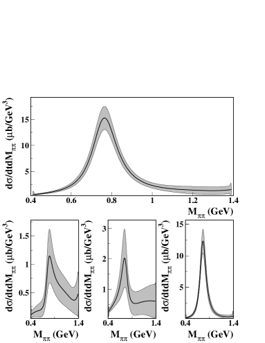
Figure 13: $P$-wave cross section derived by the fit in the $3.2<E_{\gamma}<3.4$ GeV and $0.5<-t<0.6$ GeV² bin. Bottom plots: the same amplitudes for the three possible values of $\lambda_{\pi\pi}$ (from left to right -1, 0 and +1). The systematic and fit uncertainties are added in quadrature and are shown by the gray band.

V.2 Partial wave amplitudes

The square of the magnitude of the $S$-, $P$-, $D$- and $F$-waves resulting from the fit, summed over the nucleon spin projections, is given by:

$$I_{lm}=\sum_{i=1,2}|a_{lm,i}(E_{\gamma},t,M_{\pi\pi})|^{2}.$$

When summed over the di-pion helicity, this can be written as:

$$I_{l}=\sum_{m}\sum_{i=1,2}|a_{lm,i}(E_{\gamma},t,M_{\pi\pi})|^{2},$$

where the sum is limited to $m=-1,0,1$ for $l>0$ and to $m=0$ for $l=0$.

The resulting partial wave cross sections are shown in Figs. 12, 13, 14, and 15, for a selected photon energy and $-t$ bin. The whole set of partial wave amplitudes resulting from this analysis is available at the Jefferson Lab jlab-db and the Durham dhuram-db databases.

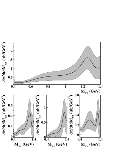
Figure 14: As Fig. 13 for $D$-wave.

As expected, the dominant contribution from the $\rho$ meson is clearly visible in the $P$-wave, whose contribution is about one order of magnitude larger than the other waves. In particular the main contribution comes from $I_{lm=1,+1}$, corresponding to a non-helicity flip ($s$-channel helicity conserving) transition. In the $S$-wave, a strong interference pattern shows up around $M_{\pi\pi}=980$ MeV, which reveals contributions from the $f_{0}(980)$ production. The contribution from the $f_{2}(1270)$ tensor meson is apparent in the $D$-wave, while no clear structures are seen in the $F$-wave.

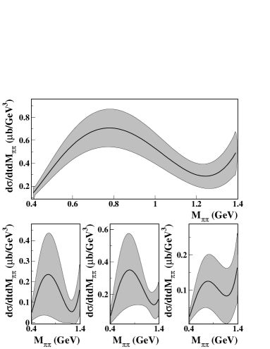
Figure 15: As Fig. 13 for $F$-wave.

V.3 Systematic studies

The error bands plotted in Figs. 12, 13, 14, and 15 include the systematic uncertainties related to the moment extraction and the photon flux normalization as discussed in Sec. III.2.3. In addition, for the $S$-wave, where the $f_{0}(980)$ contribution is strongly affected by interference, detailed systematic studies using both Monte Carlo and data were performed.

In order to test the approximation introduced by the truncation to $L_{max}$=4 in the moment extraction, we first verified the fit was able to reproduce the experimental distributions in the kinematic range of interest. Figure 16 shows the comparison between data and fit results for the decay angles in the helicity system with $M_{\pi\pi}$ in the $f_{0}(980)$ mass region ($M_{\pi\pi}=0.985\pm 0.01$ GeV). Figure 17 shows the same comparison for the invariant mass $M_{p\pi^{+}}$ when three different regions of $M_{\pi\pi}$ ($M_{\pi\pi}=0.475\pm 0.01$ GeV, $M_{\pi\pi}=0.775\pm 0.01$ GeV, $M_{\pi\pi}=1.295\pm 0.01$ GeV) were selected. The good agreement proves the accuracy of the approximation.

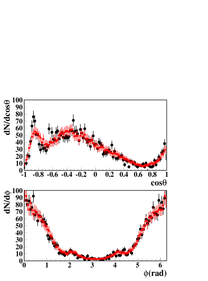
Figure 16: Pion angles in the $\pi^{+}\pi^{-}$ helicity rest frame for $M_{\pi\pi}$ in the $f_{0}(980)$ mass region ($M_{\pi\pi}=0.985\pm 0.01$ GeV). Experimental data are plotted in black and fit results in red.

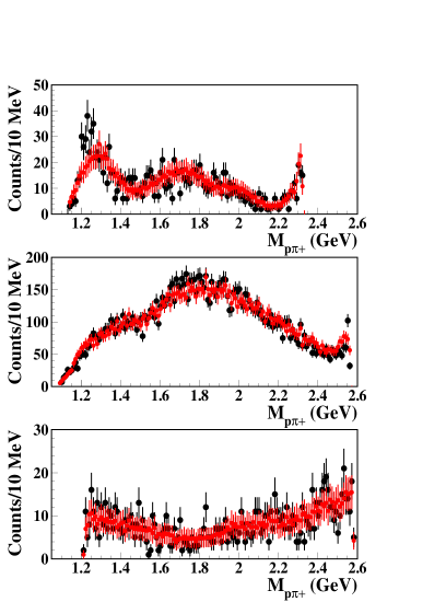
Figure 17: $M_{p\pi^{+}}$ distribution in three different $M_{\pi\pi}$ mass regions (bottom: $M_{\pi\pi}=0.475\pm 0.01$ GeV, middle: $M_{\pi\pi}=0.775\pm 0.01$ GeV, top: $M_{\pi\pi}=1.295\pm 0.01$ GeV). Experimental data are plotted in black and fit results in red.

As a second check, we applied the fit to pseudo-data obtained with a realistic event generator, processed with the CLAS GEANT-based simulation package and analyzed with the same procedure used for the data. Since the event generator was tuned to previous two-pion photoproduction measurements, it does not include any explicit limitation on the number of waves. The reconstructed moments showed that, with the chosen $L_{max}$, all fits were capable of reproducing the generated moments up to $M_{\pi\pi}\sim 1.1$ GeV. Finally, we derived a quantitative estimate of the truncation effect on the $S$-wave squared amplitude as follows. The results of a $L_{max}=8$ fit of the moments was used as input for a new Monte Carlo event generator. After being processed in the same way as discussed above, pseudo-data were fitted with $L_{max}=4$ and the $S$-wave amplitude was extracted. The difference between the generated and the reconstructed partial wave cross section was found to be of the order of 25% that, added in quadrature to the other systematic uncertainties, was included in the gray band of Fig. 12.

We also demonstrated that no structures similar to the narrow interference pattern we are interpreting as the evidence of the $f_{0}(980)$ were created by distortions induced by the CLAS acceptance. This check was performed generating events after removing the $f_{0}(980)$ contribution, and verifying that no spurious structures appeared in the spectra after the full GEANT simulation and reconstruction.

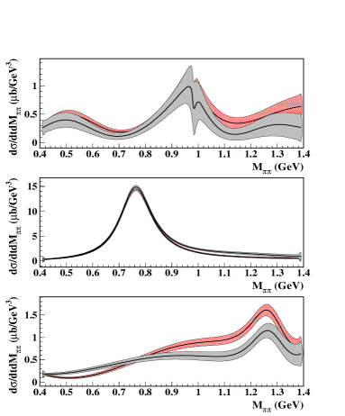
Figure 18: $S$-, $P$- and $D$-wave cross sections in the $3.4<E_{\gamma}<3.6$ GeV and $0.5<-t<0.6$ GeV² bin. The gray and red bands show the results of the standard fit and of the fit performed adding a second-order polynomial to the partial wave expansion of the moments to account for the baryon resonance contributions. The width of the bands represents the fit uncertainties only. Fit results are shown for a specific parametrization of the moments (second method, see Sec. III.2.3).

In addition, the effects of baryon resonance contributions to the di-pion mass spectrum were studied performing the fit of the moments with the inclusion of an incoherent background. In fact, the background in the di-pion mass spectrum introduced by the reflection of the baryon resonances is expected to be smooth and structureless, contributing to all waves. Therefore this was parametrized as a second-order polynomial in $M_{\pi\pi}$ that was summed to the parametrization of the moments in terms of partial waves used in the standard fits. From this study we concluded that the background contribution is small, smooth and does not affect the quality of the fit. The comparison of the fit results with and without the inclusion of this additional background indicates that the $P$-wave and the $S$-wave in the $f_{0}(980)$ region are only slightly affected, as shown in Fig. 18. On the contrary, the low mass $S$-wave, corresponding to the $\sigma(600)$ region, and the $D$-wave, corresponding to the $f_{2}(1270)$ region, show a significant variation and, therefore, a more complete analysis should be performed to extract reliable information in these mass ranges. A similar conclusion was drawn by comparing the analysis results excluding the $\Delta(1232)$, the dominant baryon resonance contribution for this final state, with the cut $M(p\pi^{+})>1.4$ GeV. A negligible effect was found on the rapid motion around the narrow $f_{0}(980)$ meson, while a larger variation was observed at higher values of the $M(\pi\pi)$ mass.

To verify the stability of the fit of moments in the region of the $f_{0}(980)$, the whole analysis was repeated reducing the $M_{\pi\pi}$ bin size from 10 to 5 MeV. The results obtained in the two cases were found to be consistent.

As a final check, the sensitivity to the specific choice of the number of terms used in the Taylor expansion of the amplitudes $\tilde{a}^{L}$ (see Eq. 19) was tested performing the partial wave analysis fits both with a second- and fourth-order polynomial. The effect was found to be negligible compared to the other systematic uncertainties.

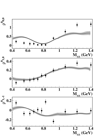
Figure 19: Spin density matrix elements for the $P$-wave in the $3.0<E_{\gamma}<3.2$ GeV and $0.4<-t<0.5$ GeV² bin. The black dots are data points from Ref. Ballam_1 , taken in a similar kinematic bin ($E_{\gamma}\sim 2.8$ GeV and $0.02<-t<0.4$ GeV²).

V.4 The spin density matrix elements

From the production amplitudes derived by the fit, we calculated the spin density matrix elements Schilling:1969um for the $P$-wave and the interference between the $S$- and $P$-waves. Some selected results are shown in Figs.  19, 20 and  21. Since these observables do not depend on the photon flux normalization, the error bands do not include the 10% uncertainty mentioned above. The whole set of spin density matrix elements resulting from this analysis is available at the Jefferson Lab jlab-db and the Durham dhuram-db databases.

Comparisons of our measurements at $3.0<E_{\gamma}<3.2$ GeV and $0.4<-t<0.5$ GeV² with existing data from Refs. Ballam_1 ; Ballam_2 in a similar kinematic domain ($E_{\gamma}\sim 2.8$ GeV and $0.02<-t<0.4$ GeV²) are shown in Fig.  19. As expected, the two matrix elements $\rho_{10}$ and $\rho_{11}$ agree very well since they have a weak dependence on $-t$, while $\rho_{00}$ shows a similar behavior, but with different values as it is more sensitive to the momentum transfer. If one compares the larger $-t$ bins we measured, the differences increase, showing that extrapolating our data to lower $-t$ would probably give good agreement with previous measurements.

As shown in Fig. 21, around $M_{\pi\pi}=980$ MeV an interference pattern clearly shows up in the $S$-$P$ wave interference term, corresponding to the contribution from the $f_{0}(980)$ meson.

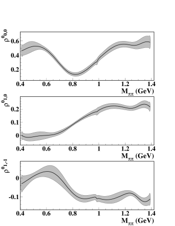
Figure 20: Spin density matrix elements for the $P$-wave in the $3.2<E_{\gamma}<3.4$ GeV and $0.5<-t<0.6$ GeV² bin.

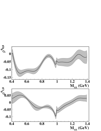
Figure 21: Spin density matrix elements for the interference between $S$- and $P$-waves in the $3.2<E_{\gamma}<3.4$ GeV and $0.5<-t<0.6$ GeV² bin.

V.5 Differential cross sections

The differential cross sections $[d\sigma/dt]_{l-wave}$ for individual waves and mass resonance regions were obtained integrating the corresponding amplitudes. The cross sections in the mass regions of the $f_{0}(980)$, $\rho$, and $f_{2}(1270)$ mesons were obtained integrating the $S$-, $P$- and $D$-waves in the mass ranges $0.98\pm 0.04$ GeV, 0.4-1.2 GeV, and $1.275\pm 0.185$ GeV, respectively. These are shown in Figs. 22, 23 and  24 in the photon energy range 3.0-3.8 GeV. As mentioned previously, the $P$-wave is completely dominated by the $\rho$ meson production, and therefore the integrated cross section can be directly compared to the world’s data for the $\gamma p\to p\rho$ reaction Battaglieri ; ABBHHM . It should be noticed that the previous cross sections were evaluated without performing a partial wave analysis but fitting the mass-dependent cross section with a relativistic Breit-Wigner plus a smooth polynomial function to separate the resonance from the background. The good agreement shown in Fig. 23 gives confidence in the partial wave analysis. As expected, the $S$-wave photoproduction is suppressed compared to the $P$-wave by more than an order of magnitude, reflecting the different mechanisms that lead to scalar and vector meson photoproduction: in Regge theory the latter is dominated by Pomeron exchange, while the former is dominated by the exchange of reggeons that become suppressed as the energy increases.

VI Summary

In summary, we have performed a partial wave analysis of the reaction $\gamma p\to p\pi^{+}\pi^{-}$ in the photon energy range 3.0-3.8 GeV and momentum transfer range $-t=0.4-1.0$ GeV². Moments of the di-pion angular distribution, defined as bi-linear functions of partial wave amplitudes, were fitted to the experimental data with an unbinned likelihood procedure. Different parametrization bases were used and detailed systematic checks were performed to insure the reliability of the analysis procedure. We extracted moments $\langle Y_{LM}\rangle$ with $L\leq 4$ and $M\leq 2$ using amplitudes with $l\leq 3$ (up to $F$-waves). Using a dispersion relation, unitarity constraint, and phase shifts and inelasticities of $\pi\pi$ scattering, the production amplitudes were expressed in a simplified form, where the unknown part was expanded in a Taylor series. The coefficients were fitted to the experimental moments to extract the $S$-, $P$-, $D$-, and $F$-waves in the $M_{\pi\pi}$ range 0.4-1.4 GeV.

Figure 22: Differential cross section $d\sigma/dt$ for the $S$-wave in the $M_{\pi\pi}$ range $0.98\pm 0.04$ GeV and photon energy range $E_{\gamma}=3.0-3.8$ GeV.

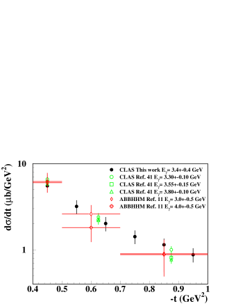
Figure 23: Differential cross section $d\sigma/dt$ for the $P$-wave in the $M_{\pi\pi}$ range 0.4-1.2 GeV and photon energy range $E_{\gamma}=3.0-3.8$ GeV.

Figure 24: Differential cross section $d\sigma/dt$ for the $D$-wave in the $M_{\pi\pi}$ range $1.275\pm 0.185$ GeV and photon energy range $E_{\gamma}=3.0-3.8$ GeV.

The moment $\langle Y_{00}\rangle$ is dominated by the $\rho(770)$ meson contribution in the $P$-wave, while the moments $\langle Y_{10}\rangle$ and $\langle Y_{11}\rangle$ show contributions of the $S$-wave through interference with the $P$-wave. The clear structure at $M_{\pi\pi}\sim 1\mbox{ GeV}$ seen in such experimental moments and in the $S$-wave amplitude is evidence of a resonance contribution that we interpret as the $f_{0}(980)$. This is the first observation of the $f_{0}(980)$ scalar meson in photoproduction. A contribution from the $f_{2}(1270)$ tensor meson was observed in the $D$-wave, while no resonant structures were seen in the $F$-wave. The cross sections of individual partial waves in the mass range of the $\rho(770)$, $f_{0}(980)$, and $f_{2}(1270)$ were computed. Finally, the spin density matrix elements for the $P$-wave were evaluated, finding good agreement with previous measurements, and for the first time, the $S-P$ interference term was extracted.

VII Acknowledgments

We would like to acknowledge the outstanding efforts of the staff of the Accelerator and the Physics Divisions at Jefferson Lab that made this experiment possible. This work was supported in part by the Italian Istituto Nazionale di Fisica Nucleare, the French Centre National de la Recherche Scientifique and Commissariat à l’Energie Atomique, the UK Science and Technology Facilities Research Council (STFC), the U.S. Department of Energy and National Science Foundation, and the Korea Science and Engineering Foundation. The Southeastern Universities Research Association (SURA) operates the Thomas Jefferson National Accelerator Facility for the United States Department of Energy under contract DE-AC05-84ER40150.

Appendix A

The explicit expressions for the moments, defined in Eq. 1 in terms of partial waves, given Eq. 4, truncated to the $L=3$ ($F$) wave are given by,

$$\langle Y_{00}\rangle = |S|^{2}+|P_{-}|^{2}+|P_{0}|^{2}+|P_{+}|^{2}+|D_{-}|^{2}+|D_{0}|^{2}+|D_{+}|^{2}+|F_{-}|^{2}+|F_{0}|^{2}+|F_{+}|^{2}$$

$$\langle Y_{10}\rangle = SP_{0}^{*}+P_{0}S^{*}+\sqrt{3\over 5}\left(P_{-}D_{-}^{*}+P_{-}^{*}D_{-}+P_{+}D_{+}^{*}+D_{+}P_{+}^{*}\right)+\sqrt{4\over 5}\left(P_{0}D_{0}^{*}+D_{0}P_{0}^{*}\right)$$

$$+ \sqrt{{24}\over{35}}\left(D_{-}F_{-}^{*}+F_{-}D_{-}^{*}+D_{+}F_{+}^{*}+F_{+}D_{+}^{*}\right)+\sqrt{{216}\over{280}}\left(D_{0}F_{0}^{*}+F_{0}D_{0}^{*}\right)$$

$$\langle Y_{11}\rangle = \left(-P_{-}S^{*}-SP_{-}^{*}+P_{+}S^{*}+SP_{+}^{*}\right)+\sqrt{1\over{20}}\left(P_{-}D_{0}^{*}+D_{0}P_{-}^{*}-P_{+}D_{0}^{*}-D_{0}P_{+}^{*}\right)$$

$$+ \sqrt{3\over{20}}\left(-P_{0}D_{-}^{*}-D_{-}P_{0}^{*}+P_{0}D_{+}^{*}+D_{+}P_{0}^{*}\right)+\sqrt{9\over{140}}\left(D_{-}F_{0}^{*}+F_{0}D_{-}^{*}-D_{+}F_{0}^{*}-F_{0}D_{+}^{*}\right)$$

$$+ \sqrt{9\over{70}}\left(-D_{0}F_{-}^{*}-F_{-}D_{0}^{*}+D_{0}F_{+}^{*}+F_{+}D_{0}^{*}\right)$$

$$\langle Y_{20}\rangle = SD_{0}^{*}+D_{0}S^{*}+\sqrt{1\over 5}\left(2|P_{0}|^{2}-|P_{-}|^{2}-|P_{+}|^{2}+|F_{-}|^{2}+|F_{+}|^{2}\right)+\sqrt{{18}\over{35}}\left(P_{-}F_{-}^{*}+F_{-}P_{-}^{*}+P_{+}F_{+}^{*}+F_{+}P_{+}^{*}\right)$$

$$+ \sqrt{{27}\over{35}}\left(P_{0}F_{0}^{*}+F_{0}P_{0}^{*}\right)+\sqrt{5\over{49}}\left(|D_{-}|^{2}+|D_{+}|^{2}\right)+\sqrt{{20}\over{49}}|D_{0}|^{2}+\sqrt{{16}\over{45}}|F_{0}|^{2}$$

$$\langle Y_{21}\rangle = {1\over 2}\left(SD_{+}^{*}+D_{+}S^{*}-SD_{-}^{*}-D_{-}S^{*}\right)+\sqrt{3\over{20}}\left(P_{0}P_{+}^{*}+P_{+}P_{0}^{*}-P_{-}P_{0}^{*}-P_{0}P_{-}^{*}\right)$$

$$+ \sqrt{9\over{140}}\left(P_{-}F_{0}^{*}+F_{0}P_{-}^{*}-P_{+}F_{0}^{*}-F_{0}P_{+}^{*}\right)+\sqrt{6\over{35}}\left(P_{0}F_{+}^{*}+F_{+}P_{0}^{*}-P_{0}F_{-}^{*}-F_{-}P_{0}^{*}\right)$$

$$+ \sqrt{5\over{196}}\left(D_{0}D_{+}^{*}+D_{+}D_{0}^{*}-D_{0}D_{-}^{*}-D_{-}D_{0}^{*}\right)+\sqrt{1\over{90}}\left(F_{0}F_{+}^{*}+F_{+}F_{0}^{*}-F_{0}F_{-}^{*}-F_{-}F_{0}^{*}\right)$$

$$\langle Y_{22}\rangle = \sqrt{3\over{10}}\left(P_{-}P_{+}^{*}+P_{+}P_{-}^{*}\right)+\sqrt{3\over{140}}\left(P_{-}F_{+}^{*}+F_{+}P_{-}^{*}+P_{+}F_{-}^{*}+F_{-}P_{+}^{*}\right)$$

$$+ \sqrt{4\over{30}}\left(-F_{+}F_{-}^{*}-F_{-}F_{+}^{*}\right)+\sqrt{3\over{196}}\left(-D_{-}D_{+}^{*}-D_{+}D_{-}^{*}\right)$$

$$\langle Y_{30}\rangle = SF_{0}^{*}+F_{0}S^{*}+\sqrt{{18}\over{70}}\left(-P_{-}D_{-}^{*}-D_{-}P_{-}^{*}-P_{+}D_{+}^{*}-D_{+}P_{+}^{*}\right)+\sqrt{{108}\over{140}}\left(P_{0}D_{0}^{*}+D_{0}P_{0}^{*}\right)$$

$$+ \sqrt{2\over{45}}\left(D_{-}F_{-}^{*}+F_{-}D_{-}^{*}+D_{+}F_{+}^{*}+F_{+}D_{+}^{*}\right)+\sqrt{{16}\over{45}}\left(D_{0}F_{0}^{*}+F_{0}D_{0}^{*}\right)$$

$$\langle Y_{31}\rangle = {1\over 2}\left(SF_{+}^{*}+F_{+}S^{*}-SF_{-}^{*}-F_{-}S^{*}\right)+\sqrt{{18}\over{140}}\left(P_{+}D_{0}^{*}+D_{0}P_{+}^{*}-P_{-}D_{0}^{*}-D_{0}P_{-}^{*}\right)$$

$$+ \sqrt{6\over{35}}\left(P_{0}D_{+}^{*}+D_{+}P_{0}^{*}-P_{0}D_{-}^{*}-D_{-}P_{0}^{*}\right)+\sqrt{1\over{90}}\left(D_{+}F_{0}^{*}+F_{0}D_{+}^{*}-D_{-}F_{0}^{*}-F_{0}D_{-}^{*}\right)$$

$$+ \sqrt{1\over{20}}\left(D_{0}F_{+}^{*}+F_{+}D_{0}^{*}-D_{0}F_{-}^{*}-F_{-}D_{0}^{*}\right)$$

$$\langle Y_{32}\rangle = \sqrt{3\over{14}}\left(-P_{+}D_{-}^{*}-D_{-}P_{+}^{*}-P_{-}D_{+}^{*}-D_{+}P_{-}^{*}\right)+\sqrt{1\over{12}}\left(-D_{+}F_{-}^{*}-F_{-}D_{+}^{*}-D_{-}F_{+}^{*}-F_{+}D_{-}^{*}\right)$$

$$\langle Y_{40}\rangle = \sqrt{2\over 7}\left(-P_{+}F_{+}^{*}-F_{+}P_{+}^{*}-P_{-}F_{-}^{*}-F_{-}P_{-}^{*}\right)+\sqrt{{16}\over{21}}\left(P_{0}F_{0}^{*}+F_{0}P_{0}^{*}\right)+\sqrt{{16}\over{49}}\left(-|D_{+}|^{2}-|D_{-}|^{2}\right)$$

$$+ \sqrt{{36}\over{49}}|D_{0}|^{2}+\sqrt{{36}\over{121}}|F_{0}|^{2}+\sqrt{1\over{121}}\left(|F_{+}|^{2}+|F_{-}|^{2}\right)$$

$$\langle Y_{41}\rangle = \sqrt{5\over{42}}\left(P_{+}F_{0}^{*}+F_{0}P_{+}^{*}-P_{-}F_{0}^{*}-F_{0}P_{-}^{*}\right)+\sqrt{5\over{28}}\left(P_{0}F_{+}^{*}+F_{+}P_{0}^{*}-P_{0}F_{-}^{*}-F_{-}P_{0}^{*}\right)$$

$$+ .\sqrt{{30}\over{196}}\left(D_{0}D_{+}^{*}+D_{+}D_{0}^{*}-D_{-}D_{0}^{*}-D_{0}D_{-}^{*}\right)+\sqrt{{30}\over{968}}\left(F_{0}F_{+}^{*}+F_{+}F_{0}^{*}-F_{0}F_{-}^{*}-F_{-}F_{0}^{*}\right)$$

$$\langle Y_{42}\rangle = \sqrt{5\over{28}}\left(-P_{+}F_{-}^{*}-F_{-}P_{+}^{*}-P_{-}F_{+}^{*}-F_{+}P_{-}^{*}\right)+\sqrt{{10}\over{49}}\left(-D_{-}D_{+}^{*}-D_{+}D_{-}^{*}\right)$$

$$+ \sqrt{{10}\over{121}}\left(-F_{-}F_{+}^{*}-F_{+}F_{-}^{*}\right)$$

It follows from Eq. 1 that the $\langle Y_{00}\rangle$ moment is normalized by the differential cross section via,

$$\langle Y_{00}\rangle=\int d\Omega_{\pi}\frac{d\sigma}{dtdM_{\pi\pi}d\Omega_{\pi}}.$$ (22)

References

(1) I. Caprini, G. Colangelo and H. Leutwyler, Phys. Rev. Lett. 96, 132001 (2006).
(2) R. Kaminski, J. R. Pelaez and F. J. Yndurain, Phys. Rev. D 77, 054015 (2008).
(3) R. Kaminski, J. R. Pelaez and F. J. Yndurain, Phys. Rev. D 74, 014001 (2006)
[Erratum-ibid. D 74, 079903 (2006)].
(4) J. R. Pelaez, Phys. Rev. Lett. 92, 102001 (2004).
(5) D. V. Bugg, Phys. Rept. 397, 257 (2004).
(6) S. Godfrey and N. Isgur, Phys. Rev. D 32, 189 (1985).
(7) H. -J. Behrend et al., Nucl. Phys. B 144, 22 (1978).
(8) D. P. Barber et al., Z. Phys C 12, 1 (1982).
(9) J. Ballam et al., Phys. Rev D 5, 545 (1972).
(10) J. Ballam et al., Phys. Rev D 7, 3150 (1973).
(11) R. Erbe et al., Phys. Rev 175, 1669 (1968).
(12) A. Airapetian et al. (HERMES Collaboration), Phys. Lett. B 599, 212 (2004).
(13) P. Söding, Phys. Lett. 19, 702 (1966).
(14) A. S. Krass, Phys. Rev. 159, 1496 (1967).
(15) G. Kramer and J. L. Uretsky, Phys. Rev. 181, 1918 (1969).
(16) J. Pumplin, Phys. Rev. D 2, 1859 (1970).
(17) T. Bauer, Phys. Rev. Lett. 25, 485 (1970).
(18) W. Struczinski et al., Nucl. Phys. B 108, 45 (1976).
(19) J. A. Gómez Tejedor and E. Oset, Nucl. Phys. A 571, 667 (1994).
(20) C-R. Ji, R. Kamiński, L. Leśniak, A. Szczepaniak, R. Williams, Phys. Rev C 58 1205 (1998).
(21) R. Kamiński, L. Leśniak, J. -P. Maillet, Phys. Rev. D 50, 3145 (1994).
(22) R. Kamiński, L. Leśniak, Phys. Rev. C 51, 2264 (1995).
(23) L. Leśniak, Acta. Phys. Pol. B 27, 1835 (1996).
(24) Ł. Bibrzycki, L. Leśniak, A. P. Szczepaniak, Eur. Phys. J. C 34, 335 (2004).
(25) A. Furman and L. Leśniak, Phys. Lett. B 538, 266 (2002).
(26) C. Wu et al., Eur. Phys. J. A 23, 317 (2005).
(27) M.Battaglieri et al. (CLAS Collaboration), Phys. Rev. Lett. 102, 102001 (2009).
(28) G. Grayer et al., Nucl. Phys. B 75, 189 (1974).
(29) H. Becker et al., Nucl. Phys. B 151, 46 (1979).
(30) C. Amsler et al. (Crystal Barrel Collaboration), Phys. Lett. B 342,
433, (1995).
(31) B.A. Mecking et al., Nucl. Instr. and Meth. A503, 513 (2003).
(32) D. I. Sober et al., Nucl. Instr. and Meth. A440, 263 (2000).
(33) S. Stepanyan et al., Nucl. Instr. and Meth. A572, 654 (2007).
(34) M. Williams, D.Applegate, and C. A. Meyer, CLAS-Note 2004-017,
http://www1.jlab.org/ul/Physics/Hall-B/clas/public/2004-017.pdf.
(35) M.D. Mestayer et al., Nucl. Instr. and Meth. A449, 81 (2000).
(36) E.S. Smith et al., Nucl. Instr. and Meth. A432, 265 (1999).
(37) Y.G. Sharabian et al., Nucl. Instr. and Meth. A556, 246 (2006).
(38) F. James and M. Roos, Computer Physics Communications 10, 343 (1975).