A population facing climate change: joint influences of Allee effects and environmental boundary geometry

Abstract

As a result of climate change, many populations have to modify their range to follow the suitable areas - their “climate envelope” - often risking extinction. During this migration process, they may face absolute boundaries to dispersal, because of external environmental factors. Consequently, not only the position, but also the shape of the climate envelope can be modified. We use a reaction-diffusion model to analyse the effects on population persistence of simultaneous changes in the climate envelope position and shape. When the growth term is of logistic type, we show that extinction and persistence are principally conditioned by the species mobility and the speed of climate change, but not by the shape of the climate envelope. However, with a growth term taking an Allee effect into account, we find a high sensitivity to the variations of the shape of the climate envelope. In this case, the species which have a high mobility, although they could more easily follow the migration of the climate envelope, would be at risk of extinction when encountering a local narrowing of the boundary geometry. This effect can be attenuated by a progressive opening of the available space at the exit of the narrowing, even though it transiently leads to a diminished area of the climate envelope.

Keywords: Allee effect $\cdot$ Biodiversity $\cdot$ Climate change $\cdot$ Climate envelope $\cdot$ Conservation $\cdot$ Mobility $\cdot$ Reaction-diffusion $\cdot$ Single species model

Introduction

Over the last century, the global Earth’s temperature has increased by about 0.7^∘C with, in the past 50 years, an even faster warming trend, of about 0.13^∘C per decade (IPCC 2007). The consequences of this warming on fauna and flora are already visible, and well documented (see e.g., Walther et al. 2002). Especially, poleward and upward shifts of many species ranges have been recorded, and are most likely linked to the climate change (Parmesan and Yohe 2003; Parmesan 2006).

The variations of Earth’s climate are in fact highly spatially heterogeneous (IPCC 2007). Thus, depending on the regions they inhabit, species may be more or less subject to high changes in climate. Some species can adapt, whereas others, and especially range-restricted species, risk extinction. A recent study based on the species-area relationships, by Thomas et al. (2004), predicted between $15\%$ and $37\%$ of species extinction in the next 50 years due to climate change, in sample regions covering $20\%$ of the Earth’s terrestrial surface.

For the next century, climate projections indeed predict a mean increase of temperature of $1.8^{\circ}$C for minimum scenarios to $4^{\circ}$C for maximum expected scenarios.

Recently, some authors proposed mathematical models for analysing the factors that influence population persistence, when facing a climate change. They used the notion of “climate envelope”, corresponding to the environmental conditions under which a population can persist. They assumed that the conditions defining this envelope did not change with time, while the envelope location moved according to climate change (Thomas et al. 2004). Keeping $0.9^{\circ}$C/100 km as the poleward temperature gradient, the above-mentioned temperature increases should imply poleward translations of the climate envelope at speeds of $2-4.5$ km/year.

A one-dimensional reaction-diffusion model has been proposed by Berestycki et al. (2007). Results have been obtained, especially regarding the links between population persistence and species mobility. Indeed, if the individuals have a too low rate of movement, then the population cannot follow the climate envelope and thus becomes extinct. On the other hand, if the individuals have a very high rate of movement, they disperse outside the climate envelope and thus the population also becomes extinct. Other related works, based on one-dimensional reaction-diffusion models, can be found in Potapov and Lewis (2004), Deasi and Nelson (2005), Pachepsky et al. (2005) and Lutscher et al. (2006).

The model that we consider here is derived from the classical Fisher population dynamics model (Fisher 1937; Kolmogorov et al. 1937). In a two-dimensional bounded environment $\Omega$, the corresponding equation is:

$$\frac{\partial u}{\partial t}=D\nabla^{2}u+ug(t,x,u),\ t\in[0,+\infty),\ x\in\Omega\subset\mathbb{R}^{2}.$$ (1)

The one-dimensional model considered by Berestycki et al. (2007) is a particular case of (1), with a logistic growth function $ug(t,x,u)$. Indeed, the authors assumed the per capita growth rate $g$ to decrease with the population density $u$ for all fixed $x$ and $t$.

Other types of growth functions are of interest, especially those taking account of Allee effect. Allee effect occurs when the per capita growth rate reaches its peak at a strictly positive population density. At low densities, the per capita growth rate may then become negative (strong Allee effect). Allee effect is known in many species (see Allee 1938; Dennis 1989; Veit and Lewis 1996). This results from several processes which can co-occur (Berec et al. 2007), such as diminished chances of finding mates at low densities (McCarthy 1997; Robinet et al. 2007b), fitness decrease due to consanguinity or decreased visitation rates by pollinators for some plant species (Groom 1998). It is commonly accepted that populations subject to Allee effect are more extinction prone (Stephens and Sutherland 1999).

In reaction-diffusion models, Allee effects are generally modelled by equations of bistable type (Fife 1979; Turchin 1998; Shi and Shivaji 2006). Mathematical analyses involving these equations have demonstrated important effects of the domain’s geometry, especially while studying travelling wave solutions. These solutions generally describe the invasion of a constant state, for instance where no individuals are present, by another constant state (typically the carrying capacity), at a constant speed, and with a constant profile (see Aronson and Weinberger 1978). Berestycki and Hamel (2006) have proved that in an infinite environment with hard obstacles, but otherwise homogeneous, travelling waves solutions of bistable equations may exist or not, depending on the shape of the obstacles. In the same idea, in an infinite homogeneous square cylinder, Chapuisat and Grenier (2005) proved that travelling wave solutions may not exist if the cylinder’s diameter is suddenly increased somewhere. See also Matano et al. (2006) for another related work. In parallel, Keitt et al. (2001), while studying invasion dynamics in spatially discrete environments, showed that Allee effect can cause an invasion to fail, and can therefore be a key-factor that determines the limits of species ranges. In one-dimensional models, Allee effect has also been shown to slow-down invasions (Hurford et al. 2006), or even to stop or reverse invasions in presence of predators (Owen and Lewis 2001), or pathogens (Hilker et al. 2005). In a study by Tobin et al. (2007), empirical evidences have also been given regarding the fact that geographical regions with higher Allee thresholds are associated with lower speeds of invasion.

The aim of this work is to study, for the simple two-dimensional reaction-diffusion model (1), how the population size variation during a shift of the climate envelope depends on the shift speed, the geometry of the environmental boundary, and on the population mobility and growth characteristics.

The first section is dedicated to the precise mathematical formulation of the model. Two types of growth functions are considered, logistic-like, or taking account of an Allee effect, with in both cases a dependence with respect to the climate envelope’s position. We define three domain types, corresponding to three kinds of geometry of the environmental boundaries. Domain 1 is a straight rectangle, and domain 2 is the union of two rectangles of same width by a narrow corridor. The comparison between domains 1 and 2 enables to analyse the effects of a local narrowing of the habitat on population persistence. As suggested by the work of Chapuisat and Grenier (2005) and Berestycki and Hamel (2006), in the case with an Allee effect, extinction phenomena may not be caused directly by the reduction of climate envelope due to the narrowing of the domain in the corridor, but by its too sudden increase at the exit of the corridor. This is why we introduced domains of type 3, which correspond to the union of two rectangles of same width by a narrow corridor, which gradually opens over a trapezoidal region of length $h$ (the case $h=0$ corresponds to domain 2). Results of numerical computations of the population size over $30$ years are presented and analysed, under different hypotheses on the growth rate, mobility, speed of climate change, and domain’s shape. These results are further discussed in the last section of this paper.

Formulation of the model

The population dynamics is modelled by the following reaction-diffusion equation:

$$\frac{\partial u}{\partial t}=D\nabla^{2}u+ug(t,x,u),\ t\in[0,+\infty),\ x\in\Omega\subset\mathbb{R}^{2}.$$

Here, $u=u(t,x)$ corresponds to the population density at time $t$ and position $x=(x_{1},x_{2})$. The number $D>0$ measures the species mobility, and $\nabla^{2}$ stands for the spatial dispersion operator $\displaystyle{\nabla^{2}u=\frac{\partial^{2}u}{\partial x_{1}^{2}}+\frac{\partial^{2}u}{\partial x_{2}^{2}}}$. The set $\Omega$ is a bounded subdomain of $\mathbb{R}^{2}$. We assume reflecting boundary conditions (also called no-flux or Neumann boundary conditions):

$$\frac{\partial u}{\partial n}(t,x)=0,\hbox{ for }x\in\partial\Omega,$$

where $\partial\Omega$ is the domain’s boundary and $n=n(x)$ corresponds to the outward normal to this boundary. Thus, the boundary of the domain $\Omega$, or equivalently the environmental boundary, constitutes an absolute barrier that the individuals cannot cross.

Growth functions

The function $g$ corresponds to the per capita growth rate of the considered species. In our model, it can be of two main types, $g_{l}$ or $g_{a}$. The first case corresponds to a logistic-like growth rate, depending on the position with respect to the climate envelope:

$$\left\{\begin{array}[]{ll}g_{l}(t,x,u)=r^{+}(1-\frac{u}{K}),&\hbox{ if }x\in\mathcal{C}(t),\\ g_{l}(t,x,u)=r^{+}(1-\frac{u}{K})-r^{-},&\hbox{ if }x\not\in\mathcal{C}(t).\end{array}\right.$$ (2)

The set $\mathcal{C}(t)\subset\Omega$ corresponds to the climate envelope at time $t$, the real number $r^{+}>0$ is the intrinsic growth rate of the species inside the climate envelope, $K$ corresponds to the carrying capacity inside the climate envelope, and $r^{-}$ corresponds to the drop in intrinsic growth rate, outside the climate envelope.

In the second case, a strong Allee effect is modelled. For fixed values of $t$ and $x$, the function $g_{a}(t,x,u)$ does not attain its maximum at $u=0$, and furthermore $g_{a}(t,x,0)<0$ for all $t>0$, $x\in\Omega$. The typical form of per capita growth term taking account of an Allee effect is

$$g_{a}=r\left(1-\frac{u}{k}\right)\left(\frac{u-c}{k}\right),$$

where $r$ is a growth term, $k$ is the environment’s carrying capacity and $c$ is the Allee threshold (see e.g., Lewis and Kareiva 1993; Keitt et al. 2001). For the comparison with the logistic case (2) to stand, we choose $r$ and $k$ such that $g_{a}(t,x,K)=g_{l}(t,x,K)=0$ for all $x\in\mathcal{C}(t)$ and

$${\max_{u\in(0,K),x\in\mathcal{C}(t)}g_{a}(t,x,u)=\max_{u\in(0,K),x\in\mathcal{C}(t)}g_{l}(t,x,u)=r^{+}}.$$

Moreover, we impose an “Allee threshold” $c$ equal to $\rho K$, for $\rho\in(0,1)$, which means that $g_{a}(t,x,u)<0$ as soon as $\displaystyle{u<\rho K}$, and for all $x\in\Omega$. Such conditions yields $k=K$ and $r=\displaystyle{\frac{4r^{+}}{(1-\rho)^{2}}}$. As in the logistic case, we assume that $g_{a}$ drops by $r^{-}$ outside the climate envelope. Finally, we obtain,

$$\left\{\begin{array}[]{ll}g_{a}(t,x,u)=r^{+}\frac{4}{(1-\rho)^{2}}\left(1-\frac{u}{K}\right)\left(\frac{u}{K}-\rho\right)&\hbox{ if }x\in\mathcal{C}(t),\\ g_{a}(t,x,u)=r^{+}\frac{4}{(1-\rho)^{2}}\left(1-\frac{u}{K}\right)\left(\frac{u}{K}-\rho\right)-r^{-}&\hbox{ if }x\not\in\mathcal{C}(t).\end{array}\right.$$ (3)

The profiles of the growth functions $ug_{l}$ and $ug_{a}$ are depicted in Figure 1, for $x$ inside and outside the climate envelope.

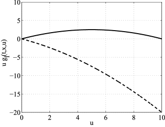
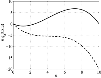
Figure 1: (a): profile of the growth rate $u\mapsto ug_{l}(t,x,u)$ inside the climate envelope ($x\in\mathcal{C}(t)$, solid line), and outside the climate envelope ($x\not\in\mathcal{C}(t)$ dashed line) in the logistic case. (b): profile of the growth rate $ug_{a}(t,x,u)$ inside the climate envelope (solid line), and outside the climate envelope (dashed line), in the case with strong Allee effect. We have set $r^{+}=1$, $r^{-}=2$, $K=10$, and $\rho=0.25$.

Throughout this paper, we make the hypothesis $r^{+}<r^{-}$.

Remark 1: In both cases, the environment’s carrying capacity is equal to $K$ inside the climate envelope. However, outside the envelope, the carrying capacity in the logistic case would be $\displaystyle{K\left(1-\frac{r^{-}}{r^{+}}\right)}$ for $r^{+}\geq r^{-}$. However, it is not defined when $r^{+}<r^{-}$. Indeed, in this last situation, the equation $ug_{l}(t,x,u)=0$ has no positive solution. Similarly, in the case with Allee effect, the equation $ug_{a}(t,x,u)=0$ has no positive solution outside the climate envelope as soon as $r^{+}<r^{-}$, since $\displaystyle{\max_{u\in(0,K),x\in\mathcal{C}(t)}g_{a}(t,x,u)=\max_{u\in(0,K),x\in\mathcal{C}(t)}g_{l}(t,x,u)=r^{+}}$. This means that the environment is not suitable for persistence outside the climate envelope.

As explained in the introduction, we assume that the climate envelope $\mathcal{C}(t)\subset\Omega$ moves poleward, according to the climate change. Assuming we are in the Northern hemisphere, we consider this move to be of constant speed $v>0$, in the second variable direction (to the “North”). Furthermore, we assume $\mathcal{C}(t)$ to be of constant thickness $L>0$:

$$\mathcal{C}(t):=\{x=(x_{1},x_{2})\in\Omega,\hbox{ such that }x_{2}\in[vt,L+vt]\}.$$

Remark 2: In this framework, the spreading speed of the population, if it survives, is constrained by the speed at which the climate envelope moves. Let us recall that, in an homogeneous one-dimensional environment, with a logistic growth rate $ur^{+}(1-u/K)$, the spreading speed is $c^{*}_{l}=2\sqrt{r^{+}D}$ (see e.g., Aronson and Weinberger 1978). In such an homogeneous environment, but with the growth rate, $4ur^{+}/(1-\rho)^{2}\left(1-u/K\right)\left(u/K-\rho\right)$, taking account of an Allee effect, the spreading speed becomes $c^{*}_{a}=2\sqrt{r^{+}D}\sqrt{2}(1/2-\rho)/(1-\rho)$ (see Lewis and Kareiva 1993). We observe that $c^{*}_{a}<c^{*}_{l}$, and that $c^{*}_{a}$ decreases with $\rho$. Thus, the spreading speed is slowed down by the Allee effect. The case $\rho=0$ corresponds to weak Allee effect: the per capita growth rate exhibits a maximum not at $u=0$, but remains positive at low densities. In that case $c^{*}_{a}[\rho=0]=c^{*}_{l}/\sqrt{2}$. The cases $\rho\geq 1/2$, corresponding to very strong Allee effects, lead to population extinction (see Lewis and Kareiva 1993).

Geometry of the environmental boundary

We work in piecewise $C^{1}$ bounded domains $\Omega$ of $\mathbb{R}^{2}$ of three different types:

1 A straight rectangle.

2 The union of two rectangles of same width by a narrow passage $\omega$.

3 The union of two rectangles of same width by a narrow passage $\omega$ followed by a trapezoidal region of height $h$.

These three domain types, and their position relatively to the origin, are depicted in Figure 2.

The domains are assumed to have a width of $20$ km (on the larger parts, for domains 2 and 3). In domains 2 and 3, the “Southern” rectangles are assumed to have a length of $40$ km. The width of the passage $\omega$ is assumed to be $2$ km, and its length $4$ km. The “Northern” environmental boundaries are situated far enough ($400$ km away from the “Southern” boundaries), so that they have no influence on the population. The climate envelope is assumed to have a latitudinal range $L=30$ km.

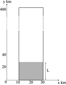
(a) Domain 1

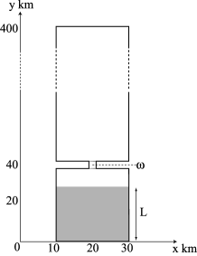
(b) Domain 2

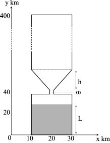
(c) Domain 3

Figure 2: Three types of domains $\Omega$. The shaded area corresponds to the climate envelope $\mathcal{C}(0)$ at $t=0$; it is represented here with a length $L=30$km. The narrow passage $\omega$ of domains 2 and 3 is separated by thin dotted lines, and is followed by a trapezoidal region of height $h$ in domain 3.

Initial condition

We assume that the population was at equilibrium, and that the climate envelope was stationary, before the considered period starting at a time $t=0$. This means that the initial condition $u(0,x)$ is a positive solution of the stationary equation:

$$-D\nabla^{2}p=p\ g(0,x,p),\ x\in\Omega\subset\mathbb{R}^{2},$$ (4)

with $\frac{\partial p}{\partial n}(x)=0$ over $\partial\Omega$. We place ourselves under the appropriate conditions for existence of such positive stationary solutions, in the logistic and Allee effect cases (see the Appendix for more details).

Results

Using a second order finite elements method, we computed the solution $u(t,x)$ of the model (1) with the growth functions and initial conditions discussed above. We focus here on the population size,

$$P(t):=\int_{\Omega}u(t,x)dx,$$

which was computed over $30$ years in various situations.

Unless otherwise mentioned, we set $r^{+}=1$ year^-1 for the intrinsic growth rate coefficient inside the climate envelope, and we assumed that the per capita growth rate was decreased by $2$ outside the climate envelope: $r^{-}=2$ year^-1. We assumed that $K=10$ individuals/km². In our computations, the diffusion coefficient $D$ varied between $1$ km²/year, corresponding to populations with low mobility, e.g., some insects species, and 50 km²/year, corresponding to populations with high mobility (see Shigesada and Kawasaki 1997, for some observed values of $D$, for different species). We first chose $\rho=0.25$, so that the Allee threshold $\rho K$ is $2.5$ individuals/km². The speeds used for the climate envelope shift varied between $v=1$ km/year and $v=6$ km/year.

Population size over time

In order to get a first insight into the general behaviour of the population size $P(t)$ for $t\in[0,30]$, we first computed it with the fixed values $v=2.5$ km/year, and $D=10$ km²/year. The results are presented in Figure 3.

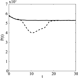
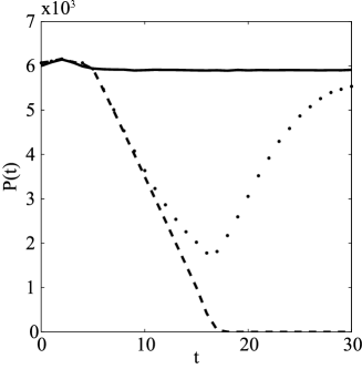
Figure 3: Computation of the populations size $P(t)$ in function of time $t$. (a) Case of the logistic growth rate $ug_{l}(t,x,u)$, in domain 1 (solid line), and in domain 2 (dashed line). (b) Case of the growth rate $ug_{a}(t,x,u)$ with Allee effect, in domains 1 (solid line), 2 (dashed line) and 3 (dotted line). For these computation, we fixed $D=10$, $v=2.5$, $r^{+}=1$, $r^{-}=2$, $K=10$, $\rho=0.25$ and $h=25$.

First notice that, as expected by our choice of growth functions, the initial population sizes, $P(0)$, are almost the same with both growth functions (2) and (3): $5800$ and $6000$ respectively in the logistic case and Allee effect case. A slight transient increase or decrease of $P(t)$, probably due to the initial effect of the Southern boundary, vanishes after $5$ years.

In domain 1, for both growth functions (2) and (3), after this short period of $5$ years, the population sizes remain stable around their initial values.

On the contrary, the populations react very differently in the domain 2, depending on the type of their growth rate. In the logistic case (Fig. 3a), the population size recovers its initial value, after a transient decrease that lasts as long as the corridor is included in the climate envelope. In the case with Allee effect (Fig. 3b), the population size declines to $0$ after $20$ years.

The behaviour of the population with Allee effect in domain 3, with $h=25$ km (Fig. 3b), leads, as in domain 2 with logistic growth, to the recovery of the initial level of population.

As a preliminary conclusion of this first step, it comes that the fate of the population will be driven by the interaction between environmental parameters ($v$ and the type of domain) and biological parameters ($D$, $r^{+}$, $r^{-}$, $K$, $\rho$, and the type of growth function).

Intertwined effects of mobility and environmental parameters

We computed the “final” population size $P(30)$, for the range of parameters $(v,D)\in(1,6)\times(1,50)$. We define the “extinction region” as the portion of the parameter space leading to $P(30)<1$.

Logistic case

The extinction region is very similar in domains 1 and 2 (Fig. 4), and corresponds to high values of $v$, and low $D$ values. In those cases, the population mobility ($D$) is not sufficient to follow the climate envelope (moving at speed $v$). In domain 1, for each value of $D$, $P(30)$ is decreasing with respect to $v$, while in domain 2, $P(30)$ is decreasing in $v$ for $v\geq 1.5$ (whenever $v<1.5$, the climate envelope has not totally crossed the corridor $\omega$ at $t=30$). As already proved in the one-dimensional case Berestycki et al. (2007), and for the same reasons recalled in the introduction section, we here observe that population sizes $P(30)$ are not monotonically linked with the parameter $D$.

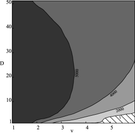
(a) domain 1

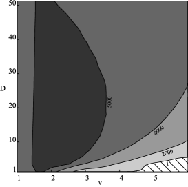
(b) domain 2

Figure 4: Logistic growth rate $ug_{l}(t,x,u)$. Contour lines of $P(30)$ in function of the speed of climate change $v$ and of the diffusion coefficient $D$, in domains 1 (a) and 2 (b). The hatched areas correspond to the extinction regions. We fixed $r^{+}=1$, $r^{-}=2$ and $K=10$.

Case with Allee effect

In domain 1 (Fig. 5a), $P(30)$ is decreasing with respect to $v$ and increasing with $D$. The extinction region again corresponds to high values of $v$, and low $D$ values. However, the extinction region is wider than in the logistic case. In domain 2 (Fig. 5b), the population does not survive as soon as $v>1.8$. The extinction region is therefore very wide compared to the one of domain 1.

Contrarily to the logistic case, a marked difference between the fate of populations in domains 1 and 2 does exist. This reflects the sensitivity to environmental boundary geometry, of populations subject to an Allee effect. In domain 3, with $h=25$, where the opening at the exit of the corridor is more progressive than in domain 2, we observe that the extinction region is reduced (Fig. 5c). It remains however larger than in domain 1, especially for large values of $D$.

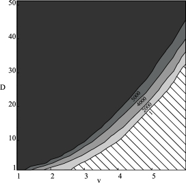
(a) domain 1

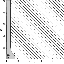
(b) domain 2

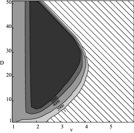
(c) domain 3

Figure 5: Case with Allee effect. (a), (b) and (c): contour lines of $P(30)$ in function of $v$ and $D$ in domains 1, 2 and 3, respectively. The hatched areas correspond to the extinction regions. For these computations, we fixed $r^{+}=1$, $r^{-}=2$, $K=10$, $\rho=0.25$ and $h=25$.

Allee effect and boundary geometry

Effect of gradual boundary change at the exit of the corridor

We have seen, in the case of population subject to an Allee effect, that domain 3, with $h=25$, gives population persistence more chances than domain 2 (which corresponds to domain 3, with $h=0$). Let us fix $v=2.5$, and see how persistence depends on $h$ and $D$. The results of the computation of $P(30)$, for $(h,D)\in[0,30]\times(1,50)$ are presented in Figure 6.

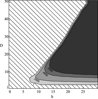
Figure 6: Case with Allee effect. Contour lines of $P(30)$ in domain 3, in function of $D$ and of the height $h$ of the trapezoidal region. The hatched area corresponds to the extinction region. The other parameters values were $r^{+}=1$, $r^{-}=2$, $K=10$, $\rho=0.25$ and $v=2.5$.

For each value of $D$, $P(30)$ increases with $h$; thus higher $h$ values give population persistence more chances. Furthermore, for each $D\geq 3$, we observe that we can define a real number $h^{*}$ such that the population goes to extinction if $h<h^{*}$, and the population survives if $h>h^{*}$. Remarkably, $h^{*}$ defines two types of geometry, characterised by the progressiveness of the opening at the exit of the corridor $\omega$, which lead to extinction or survival, respectively. For most values of $D$ ($D\geq 5$), $h^{*}$ linearly increases with $D$. For small values of $D$ ($D<3$), extinction occurs independently of the value $h$, which simply means that, as in domain 1, the population cannot follow the climate envelope shift.

These results indicate that the increased extinction risk in domain 2, compared to domain 1, may not be caused by the shrinking of the climate envelope and its fragmentation in two parts, but by the lack of progressiveness of the opening at the exit of the corridor.

Population density at the exit of the corridor governs the fate of the population

Let us focus on what happens at the exit of the corridor $\omega$. We considered the region $\Omega_{1}=\Omega\cap\{y\in(44,48)\}$, corresponding to the four kilometres following the corridor. We computed the number $P_{1}(t)=\displaystyle{\int_{\Omega_{1}}u(t,x)dx}$ of individuals in this region, and the population density $u(t,c)$ at the “centre” $\mathbf{x}_{c}$ of $\Omega_{1}$, of coordinates $(10;46)$. We compared domains 2 and 3, with the fixed parameters values $v=2.5$, $D=10$, $\rho=0.25$, and $h=25$ (which is larger than $h^{*}=10$ in this case, see Fig. 6). The results are presented in Figure 7.

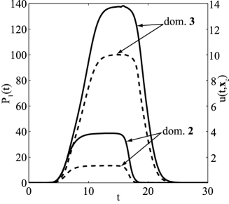
Figure 7: Case with Allee effect. Solid lines: Number of individuals $P_{1}(t)$ in the region $\Omega_{1}=\Omega\cap\{y\in(44,48)\}$, corresponding to the four kilometres following the corridor, in domains 2 and 3. Dashed lines: population density $u(t,c)$ at the “centre” $\mathbf{x}_{c}=(10;46)$ of $\Omega_{1}$. For this computation, we fixed $D=10$, $r^{+}=1$, $r^{-}=2$, $K=10$, $\rho=0.25$ and $v=2.5$.

We observe that, at the beginning of the invasion of $\Omega_{1}$, for $t\in[4,7]$, the populations $P_{1}(t)$ are almost identical in the two domains. Thus, the boundary geometry after the corridor has no effect on the number of individuals which first invade the region $\Omega_{1}$. On the contrary, during the same period of time, the population density at $\mathbf{x}_{c}$, which is situated at the exit of the corridor, remains lower in domain 2, and never reaches the Allee threshold $\rho K=2.5$. Thus, in domain 2, the dispersion of the few invaders into an open wide space, after the corridor, leads to a low population density, and therefore to a negative value of the per capita growth rate $g_{a}(t,x,u)$ (it would be false for a logistic growth function). The higher density in domain 3, for $h>h^{*}$, results from the progressiveness of the domain width offered to population development. Even if the individuals are scarce in $\Omega_{1}$, the population density at $\mathbf{x}_{c}$ exceeds the Allee threshold at $t=7$. That makes the population increase, leading to survival (survival can indeed be observed in Fig. 5c). Thus, the fate of the population seems to depend on whether or not the population density at the exit of the corridor reaches the Allee threshold.

This leads us to analyse the effect of the Allee threshold. For the same values $v=2.5$ and $D=10$, the function $\rho\mapsto h^{*}$ is presented in Fig. 8. For small values of $\rho$ ($\rho\leq 0.16$), we observe that $h^{*}=0$, i.e., the population even survives in domain 2. Then, $h^{*}$ increases with $\rho$. For higher values of $\rho$, the population never persists, at least when $h\leq 30$ (see also the end of remark 2). Finally, the stronger the Allee effect, the more progressive must be the opening at the exit of the corridor $\omega$.

On the contrary, the degree of hostility outside $\mathcal{C}(t)$, quantified by $r^{-}$, does not seem to affect much $h^{*}$. Indeed, computing $h^{*}$, for $v=2.5$, $D=10$ and $\rho=0.25$, we always obtained $h^{*}=10$, for $r^{-}\in(1,2)$ (remember that, in this work, it is assumed that $r^{-}>r^{+}$, see remark 1).

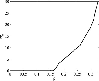
Figure 8: Case with Allee effect. Minimal value $h^{*}$ of $h$ required for persistence, in terms of the parameter $\rho$. The other parameters values were $D=10$, $r^{+}=1$, $r^{-}=2$, $K=10$ and $v=2.5$.

Discussion

Using a two-dimensional reaction-diffusion model, we have studied the fate of populations with different mobility and growth characteristics, facing environmental changes: a shift of their climate envelope, the shape of which can be modified by environmental boundary geometry.

The growth functions we considered were of two types, logistic, with a per capita growth rate modelled by (2) or taking account of a strong Allee effect (3). Boundary geometry diversity has been summarised into three schematic domain shapes (Fig. 2).

In the logistic case, the other biological parameters being fixed, the response (survival or extinction) to a climate envelope shift at speed $v$ is simply determined by the mobility of the population, which is measured by the diffusion parameter $D$. The minimum required mobility for survival increases with the speed $v$. This response is independent of the environmental boundary geometry. This clearly appeared comparing domains 1 and 2. In fact, we conjecture that it is true for any local perturbation of the boundary (it could be proved using the methods of Berestycki and Rossi, in press).

In the case with Allee effect, we observed a more complex pattern of interactions among biological and environmental parameters. In the straight domain 1, similarly to the logistic case, the higher the climate envelope shift speed, the higher the required mobility for survival. Additionally, this required mobility, at any $v$, is always higher than in the logistic case.

Facing a local narrowing of the environment, as in domain 2, contrarily to the logistic case, the chances of survival dramatically decrease in the presence of an Allee effect. In that case, high mobility is not sufficient to face climate envelope shifting at high speeds. Indeed, the population density drop at the exit of the corridor exhibits the sensitivity of this type of populations to low densities. This drop can be attenuated by a progressive opening of the available space at the exit of the corridor, as in domain 3. Even though this geometry transiently leads to a diminished area of the climate envelope, it finally results in higher chances of survival. The opening has to be all the more progressive since the Allee threshold and the species mobility are high.

Thus, a population subject to an Allee effect should have a mobility which is neither too low, in order to be able to follow the climate envelope, nor too high, in order to overcome various changes of the shape of the climate envelope. For this reason, species having an increasing dependence of their mobility with respect to their density should be more robust to climate change (see Okubo and Levin 2002, for a survey of reaction-diffusion models with density-dependent dispersal terms). On the other hand, under the environmental changes considered in this paper, populations with negatively density-dependent dispersal, such as in the model proposed by King and McCabe (2003) for the dispersal of early Palaeoindian people in North America, should have high probabilities of extinction, if an Allee effect was assumed.

The reflective boundary conditions that we used throughout this paper mean that individuals encountering the environmental boundary are reflected inside the domain. These boundary conditions can be encountered in many real-world situations, corresponding to cliffs, rivers or coasts (Shigesada and Kawasaki 1997; Jaeger and Fahrig 2004). Other boundary conditions could have been considered. With Robin boundary conditions for instance, a part of the individuals crosses the boundary. These boundary conditions write $\partial u/\partial n+\varepsilon u=0$ (see e.g., Cantrell and Cosner 2003, for some details on this type of boundary conditions). Preliminary numerical computations have shown that our results still hold in such a case, at least for small positive values of $\varepsilon$, corresponding to few individuals crossing the environmental boundary.

It was stated in Parmesan (2006), on the basis of empirical studies, that range-restricted species, like polar and mountain-top species, were at high risk of extinction induced by warming. Our study suggests that some other species may fail to expand poleward and that their capacity to expand is linked to the geometry of the geographical limits. Apart from laboratory tests under controlled conditions, the diversity of arrangements of the Alpine valleys could allow us to see whether the results of this paper can be observed in natural conditions. Indeed, insects such as pine processionary moth, the present range expansion of which is undoubtedly related to climate change (Robinet et al. 2007a), may allow us to test statistically the relationships between insect progression and the geometry of the Alpine corridors.

In this paper, a southern retraction of the climate envelope was assumed. This can be directly linked, for some species, to the fact that they are sensitive to high temperatures. This can also be caused indirectly by competition with other species, the range of which is shifting to the North. For some species, however, this retraction does not occur, leading to an expansion of the species range. This could be easily integrated in our model, by setting

$$\mathcal{C}(t):=\{x=(x_{1},x_{2})\in\Omega,\hbox{ such that }x_{2}\in[0,L+vt]\}.$$

In this case, comparable results should be obtained, with stagnation instead of extinction.

Appendix: initial conditions

When the growth rate is of logistic type, with $g=g_{l}$ satisfying (2), a sufficient condition for the existence of a positive solution $p_{l}$ of (4) can be derived by finding an appropriate sub-solution of (4) (see e.g., Amann 1976); indeed, the constant $K$ is readily a super-solution. With our choices of $\Omega$, $\mathcal{C}(0)$ and boundary conditions, for $\alpha>0$ small enough, the function

$$\phi(x,y)=\alpha\sin\left(\frac{\pi}{2}+\frac{\pi y}{2L}\right)\hbox{ for }y<L,\hbox{ and }\phi(x,y)=0\hbox{ for }y\geq L,$$

is such a sub-solution, as soon as $\frac{D\pi^{2}}{4L^{2}}<r^{+}.$ Under this condition, the function $p_{l}$ is then the unique positive and bounded solution of (4) (it can be proved as in Berestycki at al. 2005). In the logistic case, we assume that $u(0,x)=p_{l}$.

In the case (3) with Allee effect, the condition for the existence of a solution of (4), with $g=g_{a}$ is more complex, and multiple solutions may exist. However, the existence of a positive and bounded solution of (4) is still granted when $\mathcal{C}(0)$ contains a sufficiently large ball $B_{R}$. Indeed, for $R$ large enough, there exists a positive solution $\psi$ of (4) on $B_{R}$, with Dirichlet boundary conditions (Berestycki and Lions 1980). The function $\psi$, extended by $0$ to $\Omega$, is then a sub-solution of (4); the constant $K$ is again a super-solution; this implies the existence of a solution $p_{a}$ of (4) on $\Omega$. We can assume in this case that $u(0,x)=p_{a}$.

For our computations, $p_{l}$ was obtained by numerically solving (4) thanks to a second order finite elements method with triangular mesh elements. In the case with Allee effect, $p_{a}$ was computed as the limit of the solution $w(T,x)$, as $T\to+\infty$ of the initial-value problem

$$\frac{\partial w}{\partial t}-D\nabla^{2}w=w\ g(0,x,w),\ t>0,\ x\in\Omega,$$

with $w(0,x)=2K$ and $\frac{\partial w}{\partial n}(t,x)=0$ over $\partial\Omega$. The solution $w(T,x)$ was also obtained thanks to a finite elements method. The convergence of $w(T,x)$ to a positive equilibrium, as $T\to+\infty$, ensures that the condition for the existence of $p_{a}$ is fulfilled.

References

- Allee (1938) Allee WC (1938) The social life of animals. Norton, New York
- Amann (1976) Amann H (1976) Supersolution, monotone iteration and stability. J Differ Equations 21:367-377
- Aronson and Weinberger (1978) Aronson DG, Weinberger HF (1978) Multidimensional nonlinear diffusions arising in population genetics. Adv Math 30:33-76
- Berec et al. (2007) Berec L, Angulo E, Courchamp F (2007) Multiple Allee effects and population management. Trends Ecol Evol 22:185-191
- Berestycki and Hamel (2006) Berestycki H, Hamel F (2006) Fronts and invasions in general domains. C R Acad Sci Paris Ser I 343:711-716
- Berestycki and Lions (1980) Berestycki H, Lions P-L (1980) Une méthode locale pour l’éxistence de solutions positives de prolèmes semi-linéaires elliptiques. J Analyse Math 38:144-187
- Berestycki and Rossi (2008) Berestycki H, Rossi L (2008) Reaction-diffusion equations for population dynamics with forced speed I - The case of the whole space. Discret Contin Dyn S, in press
- Berestycki at al. (2005) Berestycki H, Hamel F, Roques L (2005) Analysis of the periodically fragmented environment model : I - Species persistence. J Math Biol 51:75-113
- Berestycki et al. (2007) Berestycki H, Diekmann O, Nagelkerke CJ, Zegeling PA (2007) Can a species keep pace with a shifting climate? Bull Math Biol, submitted
- Cantrell and Cosner (2003) Cantrell RS, Cosner C (2003) Spatial ecology via reaction-diffusion equations. Series In Mathematical and Computational Biology, John Wiley and Sons, Chichester, Sussex, UK
- Chapuisat and Grenier (2005) Chapuisat G, Grenier E (2005) Existence and nonexistence of traveling wave solutions for a bistable reaction-diffusion equation in an infinite cylinder whose diameter is suddenly increased. Commun Part Differ Eq 30:1805-1816
- Deasi and Nelson (2005) Deasi MN, Nelson DR (2005) A quasispecies on a moving oasis. Theor Popul Biol 67:33-45
- Dennis (1989) Dennis B (1989) Allee effects: population growth, critical density, and the chance of extinction. Natural Resource Modeling 3:481-538
- Jaeger and Fahrig (2004) Jaeger JAG, Fahrig L (2004) Effects of road fencing on population persistence. Conserv Biol 18:1651-1657
- Fife (1979) Fife PC (1979) Long-time behavior of solutions of bistable non-linear diffusion equations. Arch Ration Mech An 70:31-46
- Fisher (1937) Fisher RA (1937) The wave of advance of advantageous genes. Ann Eugenics 7:355-369
- Groom (1998) Groom MJ (1998) Allee effects limit population viability of an annual plant. Am Nat 151:487-496
- Hilker et al. (2005) Hilker FM, Lewis MA, Seno H, Langlais M, Malchow H (2005) Pathogens can slow down or reverse invasion fronts of their hosts. Biol Invasions 7:817-832
- Hurford et al. (2006) Hurford A, Hebblewhite M, Lewis MA (2006) A spatially-explicit model for the Allee effect: Why wolves recolonize so slowly in Greater Yellowstone. Theor Popul Biol 70:244-254
- IPCC (2007) Intergorvernmental Panel on Climate Change (2007) Climate change 2007: The physical science basis. Contribution of working group I to the fourth assessment report of the intergorvernmental panel on climate change. Summary for policymakers
- Keitt et al. (2001) Keitt TH, Lewis MA, Holt RD (2001) Allee effects, invasion pinning, and species’ borders. Am Nat 157:203-216
- King and McCabe (2003) King JR, McCabe PM (2003) On the Fisher-KPP equation with fast nonlinear diffusion. Proc R Soc A Math Phys Eng Sci 459:2529-2546
- Kolmogorov et al. (1937) Kolmogorov AN, Petrovsky IG, Piskunov NS (1937) Etude de l’équation de la diffusion avec croissance de la quantité de matière et son application à un problème biologique. Bull Univ Etat Moscou, Série Internationale A1:1-26
- Lewis and Kareiva (1993) Lewis MA, Kareiva P (1993) Allee dynamics and the speed of invading organisms. Theor Popul Biol 43:141-158
- Lutscher et al. (2006) Lutscher F, Lewis MA, McCauley E (2006) Effects of heterogeneity on spread and persistence in rivers. Bull Math Biol 68:2129-2160
- Matano et al. (2006) Matano H, Nakamura K-I, Lou B (2006) Periodic traveling waves in a two-dimensional cylinder with saw-toothed boundary and their homogenization limit. Networks and Heterogeneous Media 1:537-568
- McCarthy (1997) McCarthy MA (1997) The Allee effect, finding mates and theoretical models. Ecol Model 103:99-102
- Okubo and Levin (2002) Okubo A, Levin SA (2002) Diffusion and ecological problems - modern perspectives, Second edition, Springer-Verlag
- Owen and Lewis (2001) Owen MR, Lewis MA (2001) How predation can slow, stop or reverse a prey invasion. Bull Math Biol 63:655-684
- Pachepsky et al. (2005) Pachepsky E, Lutscher F, Nisbet RM, Lewis MA (2005) Persistence, spread and the drift paradox. Theor Popul Biol 67:61-73
- Parmesan (2006) Parmesan C (2006) Ecological and evolutionary responses to recent climate change. Annu Rev Ecol Evol Syst 37:637-669
- Parmesan and Yohe (2003) Parmesan C, Yohe G (2003) A globally coherent fingerprint of climate change impacts across natural systems. Nature 421:37-42
- Potapov and Lewis (2004) Potapov A, Lewis MA (2004) Climate and competition: the effect of moving range boundaries on habitat invisibility. Bull Math Biol 66:975-1008
- Robinet et al. (2007a) Robinet C, Baier P, Pennerstorfer J, Schopf A, Roques A (2007a) Modelling the effects of climate change on the potential feeding activity of Thaumetopoea pityocampa (Den. & Schiff.) (Lep., Notodontidae) in France. Global Ecol Biogeogr 16:460-471
- Robinet et al. (2007b) Robinet C, Liebhold A, Gray D (2007b) Variation in developmental time affects mating success and Allee effects. Oikos 116:1227-1237
- Shi and Shivaji (2006) Shi J, Shivaji R (2006) Persistence in diffusion models with weak Allee effect. J Math Biol 52:807-829
- Shigesada and Kawasaki (1997) Shigesada N, Kawasaki, K. (1997) Biological invasions: theory and practice. Oxford Series in Ecology and Evolution, Oxford University Press, Oxford
- Stephens and Sutherland (1999) Stephens PA, Sutherland WJ (1999) Consequences of the Allee effect for behaviour, ecology and conservation. Trends Ecol Evol 14:401-405
- Thomas et al. (2004) Thomas CD, Cameron A, Green RE, Bakkenes M, Beaumont LJ, Collingham YC, Erasmus BFN, de Siqueira MF, GraingerA, HannahL, Hughes L, Huntley B, Jaarsveld AS, Midgley GF, MilesL, Ortega-Huerta MA, Peterson AT, Phillips OL, Williams SE (2004) Extinction risk from climate change. Nature 427:145-148
- Tobin et al. (2007) Tobin PC, Whitmire SL, Johnson DM, Bjornstad ON, Liebhold AM (2007) Invasion speed is affected by geographic variation in the strength of Allee effects. Ecol Lett 10:36-43
- Turchin (1998) Turchin P (1998) Quantitative analysis of movement: measuring and modeling population redistribution in animals and plants, Sinauer Associates, Sunderland, MA
- Veit and Lewis (1996) Veit RR, Lewis MA (1996) Dispersal, population growth, and the Allee effect: dynamics of the house finch invasion of eastern North America. Am Nat 148:255-274
- Walther et al. (2002) Walther GR, Post E, Convey P, Menzel A, Parmesan C, Beebee TJC, Fromentin J-M, Hoegh-Guldberg O, Bairlein F (2002) Ecological responses to recent climate change. Nature 416:389-395