Local description of the two-dimensional flow of foam through a contraction

Abstract

The 2D flow of a foam confined in a Hele-Shaw cell through a contraction is investigated. Its rheological features are quantified using image analysis, with measurements of the elastic stress, rate of plasticity, and velocity. The behavior of the velocity strongly differs at the contraction entrance, where the flow is purely convergent, and at the contraction exit, where a velocity undershoot and a re-focussing of the streamlines are unraveled. The yielded region, characterized by a significant rate of plasticity and a maximal stress amplitude, is concentrated close to the contraction. These qualitative generic trends do not vary significantly with the flow rate, bubble area and contraction geometry, which is characteristic of a robust quasistatic regime. Using surfactants with a high surface viscoelasticity, a marked dependence of the elastic stress on the velocity is exhibited. The results show that the rate of plasticity does not only depend on the local magnitude of the deformation rate, but also crucially on the orientation of both elastic stresses and deformation rate. It is also discussed how the viscous friction controls the departure from the quasistatic regime.

1 Introduction

Liquid foams are used in many industrial and domestic applications, such as ore flotation, enhanced oil recovery or personal care. Many of these uses take advantage of the rich mechanical behavior of foams (Höhler and Cohen-Addad, 2005): under low applied strain or stress, they are elastic solids, whereas under high strain or stress, they undergo plastic flow, resulting of many elementary plastic events, the so-called T1s (Weaire and Hutzler, 1999), characterized by the topological rearrangement of four neighboring bubbles. Therefore, foams belong to the wide class of the complex fluids. Since their constitutive items, the bubbles, are of convenient size (typically $10^{-4}$ to $10^{-2}$ m) for observation, they are particularly suited to relate a macroscopic mechanical response, measured for instance by rheometry, to the microstructural behavior, which is of paramount importance to inspire or test constitutive rheological models.

Since bubbles are very efficient light scatterers, experiments on 3D foams require techniques such as Diffusive-Wave Spectroscopy (Durian et al., 1991; Gopal and Durian, 1995; Earnshaw and Wilson, 1995; Höhler et al., 1997; Vera et al., 2001) or X-ray tomography (Lambert et al., 2007). The former technique does not give precisely the bubble shape, and the latter is up to now limited by its long acquisition time. To overcome these difficulties, many experiments have been performed on bubble monolayers, the so-called quasi-2D foams (Vaz and Cox, 2005), where all bubbles can be easily imaged up to high frame rates. Since the seminal study of Debrégeas et al. (2001), many features of the flow of quasi-2D foams have been quantified, including elastic (Asipauskas et al., 2003) and plastic aspects (Dennin, 2004; Dollet and Graner, 2007), and viscous stresses (Katgert et al., 2008, 2009). This has enabled to better understand simple shear phenomena, like localization or shear-banding (Wang et al., 2006; Janiaud et al., 2006; Katgert et al., 2008; Langlois et al., 2008), although there are still open issues, such as the role of disorder (Katgert et al., 2008, 2009) and that of bubble-bubble interactions (Denkov et al., 2009). Moreover, bubble monolayers are usually confined by solid plates, except bubble rafts, and the viscous friction between bubbles and walls can drastically affect the flow profiles (Wang et al., 2006). This specificity of quasi-2D foams is a limitation for direct comparison with 3D foam flows.

Recently, tensorial constitutive models for foams, or more generally viscoelastoplastic materials (Saramito, 2007; Bénito et al., 2008; Cheddadi et al., 2008; Saramito, 2009), have been proposed in order to extend predictions of foam flows beyond pure shear (Marmottant et al., 2008). They essentially rely on a local coupling between the local magnitude and orientation of T1s, the deformation rate, and the elastic strain or stress. Therefore, to assess the validity of these tensorial models, local measurements of the elasticity, plasticity and flow profiles of foams flowing in complex geometries is required. However, such flows have been less investigated than simple rheometric flows: some experiments have focused on flows past obstacles either in 3D (Cantat and Pitois, 2006) or in 2D (Dollet et al., 2005, 2006), and some studies have reported on foam flows through contractions (Earnshaw and Wilson, 1995, 1996; Asipauskas et al., 2003; Bertho et al., 2006). Earnshaw and Wilson (1995, 1996) have shown that the rate of plastic events is globally proportional to the local rate of strain, consistently with pure shear configurations (Gopal and Durian, 1995), but in the absence of in-situ measurements of bubble deformation, the role of the elastic stress remains unclear. Hence, the existing studies have not provided a complete enough description of the flow to constitute stringent tests for the models.

To help filling this gap, in this paper, a characterization of the rheological response of a quasi-2D foam flowing towards, through, and out a contraction is proposed. We introduce the experimental setup and the methods of image analysis in Sec. 2. We then describe in details a “reference” experiment, quantifying the elastic and plastic behaviors of the foam, and its flow profile (Sec. 3). Several control parameters are then investigated, such as the flow rate, bubble size, contraction geometry and interfacial properties of the used surfactants (Sec. 4). We finally discuss and explain the complex interplays between elasticity, plasticity and flow, and between surface and bulk rheologies (Sec. 5), which make this configuration suited to shed insight on foam rheology.

2 Materials and methods

2.1 Experimental setup

We have used the foam channel fully described in Cantat et al. (2006). It is a Hele–Shaw cell, made of two horizontal glass plates of length 170 cm and width 32 cm, separated by a gap $h=2$ mm thin enough that the foam is confined as a bubble monolayer (Fig. 1a). To make the contraction, home-made plastic plates were designed. They are long, narrow plates with a central wider part, which constitutes the contraction itself (Fig. 1b). Three pairs were made, with different contraction lengths $\ell_{c}$ (2, 5 and 15 cm; the corresponding lengths $L$ are 35, 33.5 and 28.5 cm). These plates are inserted in the channel through its open end, such that the distance between the contraction and the channel exits is 30 cm. This enables to change easily the contraction width $w$. Its maximal value is 4.4 cm when the plates are in contact with the channel side walls, and we studied also widths of 3.2, 2.1 and 1.0 cm, for which a small gap remains between the channel side walls and the plates (Fig. 1b). The corresponding aspect ratios $W/w$, with $W$ the channel width upstream and downstream the contraction, are 4.6, 6.0, 8.6 and 19. The dimensions and the alignment of the two plates of a given pair are within 1.5 mm, as can be seen in Fig. 1c.

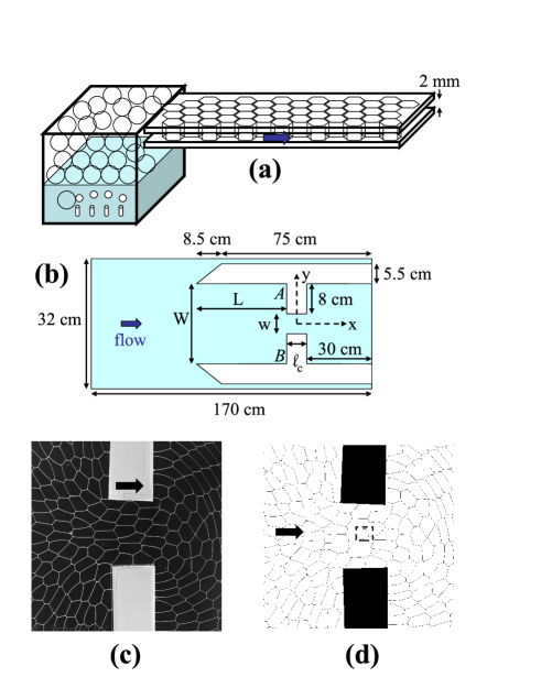
Figure 1: (a) Side view of the setup (without the contraction plates). (b) Top view (not to scale) of the foam channel and the contraction plates. Only the invariant dimensions have been indicated. The streamwise axis $x$, and the spanwise axis $y$, originating from the contraction center, are also drawn in dashed lines. (c) Snapshot of a foam flowing through a contraction of length 2.0 cm and width 3.2 cm. (d) Skeletonized version of snapshot (c), used for image analysis. The dashed rectangle is one of the boxes over which velocity, elastic stresses and plastic events are counted (see Sec. 2.2). The flow direction is depicted by the bold arrows in each subfigure.

The channel is connected upstream to a vertical chamber (Fig. 1a) in which a given amount of soap solution is introduced thanks to a peristaltic pump. Nitrogen is continuously blown through injectors at the bottom of this chamber, producing rather monodisperse bubbles (Fig. 1c) in the flow rate operating range of the paper (less than 150 ml/min per injector). The flow rate in each injector is independently controlled with an electronic flow-rate controller (Brooks). The resulting foam accumulates on top of the chamber, over a vertical distance where it drains, then is pushed through the channel. The transit time through the whole channel is less than 10 minutes in all experiments; we did not observe significant change of bubble size during this time, hence coarsening is negligible. The level of the foam/solution interface in the chamber was kept constant (within 2 mm) in all experiments to minimize the variations of liquid fraction. The latter is very low (Fig. 1c) and difficult to measure with precision. We can only give a rough estimate based on the decrease of the level of the foam/solution interface, which gives the volume of solution evacuated from the vertical chamber within the flowing foam. Comparing this volume with the gas flow rate, we get a liquid fraction between 0.2% and 0.4% for the experiments presented in this paper.

In order to change the surface rheology, two different solutions were used. Most of the experiments were done with a solution of SDS (Sigma-Aldrich; purity $>99.0\%$) dissolved in ultra-pure water (Millipore) at a concentration of 10 g/l, above the critical micellar concentration (cmc) of 2.3 g/l. Its surface static and dynamic properties were measured with a tensiometer (Teclis). We measured by the rising bubble method a the surface tension $\gamma=36.8\pm 0.3$ mN/m. Using the oscillating bubble method, we measured a total dilatational surface modulus, defined as $E_{S}=|\mathrm{d}\gamma/\mathrm{d}\ln A|$ with $A$ the bubble area, below the noise level, hence lower than 1 mN/m: as expected, pure SDS interfaces have a negligible viscoelasticity and can be considered as fully “mobile” (Denkov et al., 2005). All SDS solutions were used within a day from fabrication. Conversely, to study the case highly viscoelastic or “rigid” interfaces, we used a mixture of SLES, CAPB and myristic acid (MAc), following the protocol described in Golemanov et al. (2008): we prepare a concentrated solution of 6.6% wt of SLES and 3.4% of CAPB in ultra-pure water, we dissolve 0.4% wt of MAc by continuously stirring and heating at 60^∘C for about one hour, and we dilute 20 times in ultra-pure water. The solution has a surface tension of $22.0\pm 0.5$ mN/m, and a surface modulus of 216 mN/m for a frequency of 0.2 Hz and a relative area variation $\delta S/S_{0}=1.0\%$. Although it fully ensures that the interfaces are in the “rigid” limit (Denkov et al., 2005), this value is somewhat lower than that measured by Golemanov et al. (2008), which is $E_{S}=305$ mN/m. This likely comes from the fact that these authors have used a piezoelectric control of the bubble oscillations, which was shown to be of better accuracy to impose sinusoidal area variations than our syringe-driven control, especially for interfaces of high surface modulus (Russev et al., 2008). As Golemanov et al. (2008), we measured a significant decrease of the surface modulus with increasing relative area variation (data not shown). Both solutions have a bulk viscosity equal to that of water, $\mu=10^{-3}$ Pa s.

The contraction region is lit by a circular neon tube of diameter 40 cm, placed just below the channel on a black board. It gives an isotropic and nearly homogeneous illumination over a diameter of about 20 cm. Movies of the foam flow are recorded with the high-speed camera APX-RS (Photron) at a frame rate of 60 or 125 frames per second, with a short shutter speed of 1 ms, so that even the fastest bubbles (more than 10 cm/s) remain sharp. For all experiments except the ones with varying width (Sec. 4.2) and surfactants (Sec. 4.3), we have recorded two movies, one upstream and one downstream the contraction, to record the flow far enough the contraction. The movies are constituted of 1000 images constituted by $1024\times 1024$ pixels.

2.2 Image analysis

To extract the relevant rheological information from the movies, we follow a procedure very similar to that presented in Dollet and Graner (2007). First, each image of the movie is thresholded and skeletonized with a custom ImageJ macro. Since the foam is very dry and therefore the liquid films are thin, the shape of the bubbles is well preserved (Fig. 1d), contrary to wet foams (Dollet and Graner, 2007). As an important consequence, the elastic stress, based on the network of bubble edges, can be precisely estimated. The bubbles touching the contraction plates (sketched in white in Fig. 1b) are less well preserved, because of the uncertainty on the location of these plates; notably, their area is often underestimated. Therefore, we will discard most of the information close to the contraction plates. Second, the skeletonized movie is analyzed by a custom Delphi program fully described in Dollet and Graner (2007); based on individual bubble, edge and vertex tracking, it enables to compute the velocity, elastic stress and plastic events over a rectangular mesh of $30\times 30$ boxes covering each image. The area of each box is comparable with the bubble area (Fig. 1d), but the average over the 1000 images of each movie ensures that the fields are smooth at such a length scale. For the sake of clarity, the maps of the various fields presented in this paper are recomputed and displayed at a coarser scale.

The velocity is computed by averaging every bubble displacement over consecutive images. We will plot it both as a vector field $\vec{v}$, and as a streamline plot. We also compute the deformation rate tensor $\bar{\bar{D}}=(\overline{\overline{\nabla v}}+{{}^{t}}\overline{\overline{\nabla v}})/2$, where ^t designs matrix transpose.

To compute the elastic stress (Batchelor, 1970), we use the specific definition valid for 2D foams (Janiaud and Graner, 2005):

$$\bar{\bar{\sigma}}=\lambda\rho\left\langle\frac{\vec{\ell}\otimes\vec{\ell}}{\ell}\right\rangle,$$ (1)

with $\lambda$ the effective line tension (i.e. the pulling force exerted by each bubble edge), $\rho$ the areal bubble edge density, $\vec{\ell}$ the notation for the vector joining two neighboring vertices (the edge curvature is neglected in the above expression of the elastic stress), and $\otimes$ the tensorial product: in components $\alpha,\beta=x,y$, Eq. (1) can be rewritten as $\sigma_{\alpha\beta}=\lambda\rho\langle\ell_{\alpha}\ell_{\beta}/\ell\rangle$. Each bubble edge is constituted of a thin liquid film separated by two parallel vertical interfaces, between two Plateau borders in contact with the top and bottom walls. Since the foam is dry, the Plateau borders are of much smaller size than the gap, so we take the approximation: $\lambda\simeq 2\gamma h$. Concerning the edge density, since in average a bubble has six edges, we take $\rho=3/A$ with $A$ the average bubble area. The elastic stress, a purely mechanical notion, is strongly correlated to the purely geometrical notion of bubble (elastic) deformation, as was proposed in Aubouy et al. (2003) and shown in various experimental cases (Asipauskas et al., 2003; Janiaud and Graner, 2005; Marmottant et al., 2008); hence, we may hereafter interpret some features of the elastic stress in terms of bubble deformation. By definition, the elastic stress is a symmetric tensor with positive eigenvalues; hence, it is represented as an ellipse which major (minor) axis is proportional to the highest (lowest) eigenvalues and oriented along the corresponding eigenvectors.

The T1s are tracked as described in Dollet and Graner (2007). For the four bubbles concerned by a T1, we denote $\vec{r}_{d}$ the vector linking the centers of the two bubbles that lose contact, and $\vec{r}_{a}$ the vector linking the centers of the two bubbles that come into contact, and we ascribe this information to the box where the event takes place. In our routine, the research of appearing and disappearing contacts are run independently; therefore, to ensure that it is a relevant way to characterize T1s, we have checked that the number of disappearing ($N_{d}$) and appearing ($N_{a}$) edges is equal (within 10%) in each box. We thus compute the scalar field of the frequency of T1s per unit time and area:

$$f_{T1}=\frac{N_{a}+N_{d}}{2A_{\mathrm{box}}t_{\mathrm{movie}}},$$

where $A_{\mathrm{box}}$ is the area of a box and $t_{\mathrm{movie}}$ the duration of a movie.

As a limitation of our approach, we cannot measure the pressure field. Laplace law, which states that the pressure differences between two neighboring bubbles is proportional to the curvature of their common edge, cannot be used here: it requires to know the full 3D geometry of the bubbles, whereas the out-of-plane edge curvature is lost during our purely 2D image analysis. Furthermore, Laplace law is strictly valid only at equilibrium, and its applicability to flow situations is questionable. Nevertheless, we verified in the reference experiment that the flow rate across various cross-sections remains constant (within 4%), which is a signature of an incompressible flow. Since the trace of the deformation rate tensor, $\vec{\nabla}\cdot\vec{v}$, is zero for such a flow, the deformation rate is a symmetric and (almost) traceless tensor, hence it has a positive and a negative eigenvalue: we represent two orthogonal lines, a thick (thin) one in the direction of the eigenvector associated to the positive (negative) eigenvalue, i.e in the direction of local elongation (compression) rate, as in Dollet and Graner (2007).

3 Study of a reference experiment

We now study in detail a reference experiment. It is a flow of a SDS foam, at flow rate 150 ml/min, in a contraction of length 2 cm and width 3.2 cm. The average bubble area is 39 mm², and the polydispersity index, defined as the standard deviation of the list of individual bubble areas, is 22%, but 90% of the bubbles are within 3% from the average area, the rest being constituted mainly of much smaller bubbles. Hence, the foam is rather monodisperse (Fig. 1c).

We describe the main features of each field (velocity, Sec. 3.1; elastic stress, Sec. 3.2 and T1s, Sec. 3.3) on the maps, and we report the evolution of the different components of each field along different axes: the central axis $y=0$; an off-centered, spanwise axis located half-way between the central axis and the side walls, i.e. at $|y|=4.8$ cm, with an average over the axes $y=-4.8;$ cm and $y=4.8$ cm; a spanwise axis across the flow upstream the contraction, at $x=-9.6$ cm; and the symmetric spanwise axis downstream the contraction, at $x=9.6$ cm. For the two latter axes, since $y=0$ is an axis of symmetry, the fields will be plotted for $|y|\geq 0$, with an average over $-y$ and $y$.

3.1 Velocity

The velocity field and the streamlines are plotted in Fig. 2 and the velocity components along the different axes are plotted in Fig. 3. The foam tends towards a plug flow far from the contraction, and is faster close to the contraction, as can be seen from the velocity variation along the central axis (Fig. 3a). We do not evidence any dead zones, nor vortices, in the corners at the entrance side (denoted by letters A and B in Fig. 1b); the bubbles keep flowing towards the contraction even in the corners. This is a qualitative difference with pure viscoplastic fluids, where dead zones or vortices are observed in the corners at the entrance side (Abdali et al., 1992; Jay et al., 2002). Moreover, several features show that the flow displays a strong fore-aft asymmetry with respect to the contraction center. First, the flow along the channel walls $y=1$ cm is faster than along the channel walls $y=-1$ cm. Second, whereas the flow is purely convergent towards the contraction at the entrance zone, i.e. $v_{y}$ has always the opposite sign as $y$ (Fig. 3c), it is not purely divergent at the exit: Fig. 2 shows that any streamline passes by a maximum distance from the central axis, before converging again towards the center. This reversal of the spanwise velocity component is clearly seen in both on an off-centered streamwise axis (Fig. 3b) and across a spanwise axis in the exit region (Fig. 3d). Third, whereas the streamwise component of velocity along the central axis continuously increases towards the contraction in the entrance region, it passes through an undershoot (at $x=10$ cm) in the exit region (Fig. 3a); at this point, $v_{x}$ is 20% lower than the plug flow velocity. Furthermore, whereas the streamwise velocity component decreases from the central axis to the sides in the entrance region (Fig. 3c), it increases in the exit region and almost doubles from the central axis to the sides (Fig. 3d). We finally notice that along the central axis, $v_{y}$ slightly deviates from the zero value expected from symmetry. This is likely due the small geometric imperfections of the contraction (Sec. 2.1 and Fig. 1c).

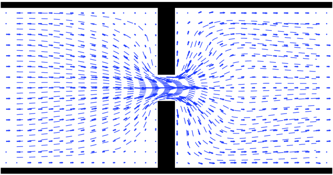
Figure 2: Velocity field and streamlines for the reference experiment. The points where the velocity could not be reliably evaluated are left in blank. The streamlines starting close to the contraction plates are interrupted in zones where the velocity could not be reliably evaluated.

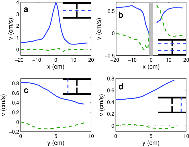
Figure 3: Plots of the velocity components $v_{x}$ (plain curve) and $v_{y}$ (dashed curve) along (a) the central axis $y=0$, (b) the off-centered axis $y=4.8$ cm, (c) upstream the contraction, along the axis $y=-9.6$ cm, and (d) downstream the contraction, along the axis $y=9.6$ cm.

3.2 Elastic stress

The map of elastic stress is presented in Fig. 4a. Not surprisingly, the maximal stress is directed towards the contraction at the entrance region, because the bubbles tend to be deformed by the converging flow. The situation is more complex at the exit region: the bubbles relax and revert their elastic stress very abruptly just at the contraction exit, and they are strongly stressed along the orthoradial direction (from the contraction center) up to a few centimeters downstream the contraction, before experiencing a gradual elastic relaxation towards equilibrium, which is not finished as they are advected away from the observation window. As a specific feature of the setup, Fig. 4b shows that the foam is prestressed at the upstream end of the observation window; indeed, the foam has passed a first contraction from the main foam channel (of width 32 cm) to the channel of width $W$ (Fig. 1) 15 cm only before the upstream end of the observation window, hence it probably did not relax completely before arriving in the field of view.

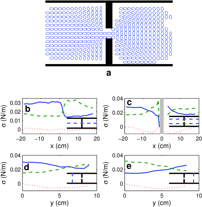
Figure 4: (a) Elastic stress field for the reference experiment. The major (minor) axis represents the local direction and magnitude of maximal (minimal) stress, see Sec. 2.2. The points where the elastic stress could not be reliably evaluated are left in blank. Plots of the elastic stress components $\sigma_{xx}$ (plain curve), $\sigma_{xy}$ (dotted curve) and $\sigma_{yy}$ (dashed curve) along (b) the central axis $y=0$, (c) the off-centered axis $y=4.8$ cm, (d) upstream the contraction, along the axis $y=-9.6$ cm, and (e) downstream the contraction, along the axis $y=9.6$ cm.

3.3 T1s

We now turn to the plastic rearrangements T1s. The spatial distribution of their frequency is plotted in Fig. 5a. It shows that plasticity occurs rather close to the contraction, within a radius of 7 cm. This is confirmed by Figs. 5b, c, d and e: there are about 5 times less T1s along the off-centered streamwise axis than along the central axis, and more than 10 times less across the spanwise axes located 9.6 cm from the contraction center. As an immediate consequence, the foam behaves as a viscoelastic medium outside this zone, which confirms that the features reported farther downstream (re-focussing of the streamlines towards the central axis, velocity undershoot) are likely due to the elastic nature of the foam. Fig. 5a and b show that there are more T1s at the entrance than at the exit of the contraction; however, this may be a specific result of the setup due to the prestress of the foam arriving in the contraction, which facilitates the occurrence of T1s. The distribution of T1s displays more generic fore-aft asymmetries: there are significant secondary maxima close to the corners in the exit region, and not in those of the entrance region; and, remarkably, there is a small zone of negligible plasticity just at the exit of the contraction (Fig. 5a and b), which we will describe further in Sec. 5.

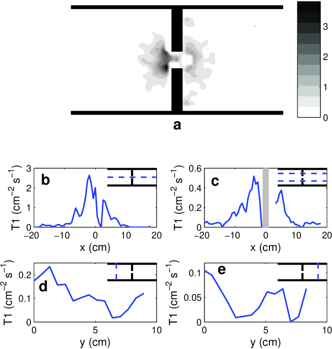
Figure 5: (a) Spatial distribution of the frequency of T1s, $f_{T1}$, expressed in cm${}^{-2}\cdot$s^-1, for the reference experiments. Plots of the frequency of T1s along (b) the central axis $y=0$, (c) the off-centered axis $y=4.8$ cm, (d) upstream the contraction, along the axis $y=-9.6$ cm, and (e) downstream the contraction, along the axis $y=9.6$ cm.

4 Influence of control parameters

We now study the influence of several control parameters on the flow of foam through a contraction. Starting from the reference experiment studied in Sec. 3, we show that a change in flow rate and in bubble area does not modify the velocity and elastic stress, up to a rescaling by the flow rate and bubble area, respectively (Sec. 4.1). We then study the influence of the length and width of the contraction (Sec. 4.2). We finally show how the physico-chemistry, i.e. the used surfactants, can affect the foam response in velocity and elastic stress (Sec. 4.3). A summary of the various experiments, and their main characteristics: applied flow rate, maximal velocity, soap solution, mean bubble area, polydispersity, contraction width $w$ and length $\ell_{c}$, is displayed in Tab. 1.

Sec.	flow rate	maximal	solution	mean bubble	polydispersity	$w$	$\ell_{c}$
	(ml/min)	velocity (cm/s)		area (mm2)	index (%)	(cm)	(cm)
3	150	3.97	SDS	39	22	2.0	3.2
4.1	75	2.01	SDS	28	36	2.0	3.2
4.1	$2\times 150$	7.38	SDS	38	25	2.0	3.2
4.1	$2\times 75$	3.90	SDS	29	44	2.0	3.2
4.2	150	7.00	SDS	33	23	2.0	1.0
4.2	150	5.35	SDS	31	38	2.0	2.1
4.2	150	3.09	SDS	35	34	2.0	4.4
4.2	150	3.90	SDS	33	15	5.0	3.2
4.2	$3\times 150$	9.84	SDS	34	36	15.0	3.2
4.3	20	0.26	*	19	36	2.0	3.2
4.3	40	0.58	*	19	36	2.0	3.2
4.3	70	1.02	*	19	36	2.0	3.2

Table 1: Summary of the main characteristics of the experiments presented in this paper. The star designs the SLES/CAPB/MAc solution described in Sec. 2.1. The fluid fraction is comprised between 0.2% and 0.4% in all experiments (Sec. 2.1).

4.1 Flow rate and bubble area: flow rescaling

To study the influence of the applied flow rate starting from the reference experiment of Sec. 3, for which the gas was injected through a single injector at a flow rate of 150 ml/min, we used a second injector through which gas is injected at the same flow rate, independently controlled by a second flow-rate controller. To study the influence of the bubble area at the reference flow rate of 150 ml/min, since the flow rate per injector is the key parameter to tune the bubble size, we blow gas through the two injectors at 75 ml/min each. We also performed an experiment with a single injector blowing at 75 ml/min. Note that we were limited to a narrow range of parameters by the number of injectors bubbling identically.

To compare these four experiments, we focus on the variations on the central axis of the relevant components of the fields, properly rescaled. For the velocity, we take $v_{x}/v_{0}$, where $v_{0}$ is the entrance velocity, i.e. the velocity averaged over a cross-stream section at the upstream end of the field of view. For the 75, 150, $2\times 75$ and $2\times 150$ experiments, we found respectively entrance velocities of 0.29, 0.58, 0.62 and 1.15 cm/s. For the elastic stress, the relevant components are the normal components $\sigma_{xx}$ and $\sigma_{yy}$. We will consider the normal stress difference $\sigma_{xx}-\sigma_{yy}$. Since the elastic stress scales as a bubble characteristic length, we rescale the normal stress difference by the trace $\sigma_{xx}+\sigma_{yy}$, to compare different bubble areas.

We thus plot along the central axis $v_{x}/v_{0}$, $(\sigma_{xx}-\sigma_{yy})/(\sigma_{xx}+\sigma_{yy})$ and the T1 frequency for the four experiments, in Fig. 6. Fig. 6a shows that all data for the rescaled velocity collapse on a single master curve; notably, the velocity undershoot at $x=10$ cm is a robust observation. Fig. 6b shows that the rescaling is good also for the dimensionless normal stress difference, within slightly larger, but apparently random, deviations from the main trend. Since the elastic stress depends on individual bubble sizes, this may be due to the small variations of polydispersity between the different runs. However, we consistently observe the same variations of the dimensionless normal stress difference along the central axis: a small increase, then a plateau close to the contraction entrance, followed by a quick reversal just at the contraction exit followed by an elastic relaxation. Finally, the T1 frequency shows consistently two peaks, one higher at the entrance and one smaller at the exit, separated by a narrow zone with negligible plasticity just at the exit of the contraction (Fig. 6c). The T1 frequency for the $2\times 75$ and $2\times 150$ experiments is about the same, and is then lower for the 150 experiment, and even lower for the 75 experiment. This suggests that the T1 frequency increases as the velocity increases and the bubble size decreases, and dimensionally, we could expect that $f_{T1}\propto v/A^{3/2}$. But if this relation holded, the ratio of the T1 frequency of the $2\times 150$ and $2\times 75$ experiments would equal 2, whereas Fig. 6c shows that they are almost equal. Hence, there is no obvious scaling for the T1 frequency.

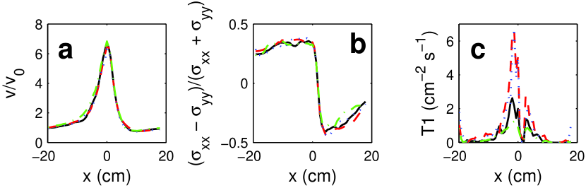
Figure 6: Comparison between different flow rates and bubble areas: in terms of number of injectors times the flow rate per injector (which specifies see bubble area, see text for details) 150 ml/min (reference experiment, plain curve), $2\times 150$ ml/min (dashed curve), $2\times 75$ ml/min (dotted curve), and $75$ ml/min (dash-dotted curve). Plots along the central axis $x=0$, of (a) the streamwise velocity component rescaled by the entrance velocity (see text for details), $v_{x}/v_{0}$, (b) the normal stress difference rescaled by the total elastic stress, $(\sigma_{xx}-\sigma_{yy})/(\sigma_{xx}+\sigma_{yy})$, and (c) the frequency of T1s.

4.2 Geometric parameters

We now describe the influence of the geometric parameters of the contraction itself, i.e. its width and length. First of all, starting from the reference experiment of Sec. 3, we have changed only the width, and studied four values of it: 1.0, 2.1, 3.2 (reference case) and 4.4 cm. As in the reference experiment, we have used one injector at 150 ml/min.

As in Sec. 4.1, a proper rescaling is useful to compare data on the velocity and elastic stress. A reference velocity based on the common flow rate of 150 ml/min is irrelevant, since as the contraction width changes, there is a varying gap between the contraction plates and the channel side walls (Fig. 1) hence a varying “leakage” flow rate through this gap. Moreover, for these experiments, we have recorded only one movie each, centered on the contraction, hence we resolve the flow on a narrower range up- and downstream the contraction ($|x|<9$ cm) and we cannot estimate an entrance velocity in a plug flow regime as in Sec. 4.1. Therefore, we take as reference velocity the maximal velocity (see Tab. 1 for values), which is reached at the contraction center for these four experiments. Since the average area varies between the different runs (Tab. 1), we also rescale the stress as in Sec. 4.1. From the results of last Section, we expect differences between the four experiments to be purely due to the width variation. Hence, we plot $v_{x}/v(x=0)$, $(\sigma_{xx}-\sigma_{yy})/(\sigma_{xx}+\sigma_{yy})$ and the T1 frequency along the central axis for the four experiments, in Fig. 7.

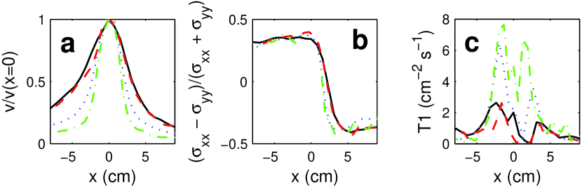
Figure 7: Comparison between different contraction widths, at the reference flow rate and bubble area: 1.0 cm (dashed curve), 2.1 cm (dotted curve), 3.2 cm (reference case, plain curve) and 4.4 cm (dash-dotted curve). Plots along the central axis $x=0$, of (a) the streamwise velocity component rescaled by the maximal velocity, $v_{x}/v(x=0)$, (b) the normal stress difference rescaled by the total elastic stress, $(\sigma_{xx}-\sigma_{yy})/(\sigma_{xx}+\sigma_{yy})$, and (c) the frequency of T1s.

The modification of the width does not alter the qualitative trends of the fields. As before, the velocity passes by a maximum in the contraction (and we miss here the undershoot, too far away downstream), the stress reverses in the contraction, and the T1 frequency shows two peaks at the entrance and at the exit, the former being slightly higher than the latter. Basically, the smaller the width, the more abrupt the velocity and stress variations across the contraction, and the higher the maxima in the T1 frequency distribution, which is coherent since the deformation rate increases.

Second, using different pairs of plates, we have varied the length of the contraction: from 2 cm (reference case), to 5 and 15 cm. The width is maintained at the reference value of 3.2 cm. As for the different widths, we choose to rescale the velocity by $v(x=0)$, equal to 3.97, 3.90 and 9.84 cm/s respectively for the lengths 2, 5 and 15 cm, and we plot $v_{x}/v(x=0)$, $(\sigma_{xx}-\sigma_{yy})/(\sigma_{xx}+\sigma_{yy})$ and the T1 frequency along the central axis for the three experiments, in Fig. 8.

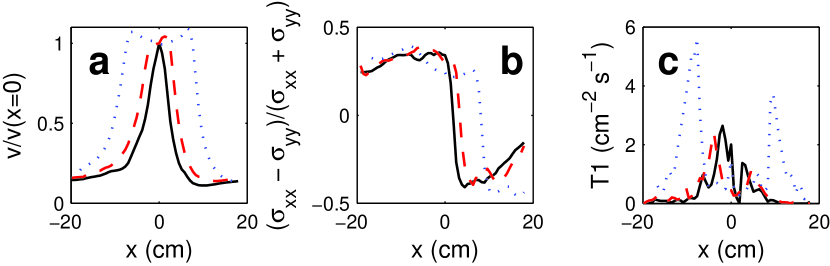
Figure 8: Comparison between different contraction lengths, at the reference flow rate, bubble area and width: 2 cm (reference case, plain curve), 5 cm (dashed curve) and 15 cm (dotted curve). Plots along the central axis $x=0$, of (a) the streamwise velocity component rescaled by the velocity at the middle of the contraction, $v_{x}/v(x=0)$, (b) the normal stress difference rescaled by the total elastic stress, $(\sigma_{xx}-\sigma_{yy})/(\sigma_{xx}+\sigma_{yy})$, and (c) the frequency of T1s.

Fig. 8a shows a new interesting feature: for long enough contractions, the velocity is not maximum anymore at the center of the contraction, as was the case up to now for the “short” contraction of 2 cm. Namely, for a contraction length of 5 cm, the velocity is maximum at $x=1.3$ cm, close to the contraction exit. For a contraction length of 15 cm, two velocity overshoots appears, at the entrance ($x=-6.0$ cm) and exit ($x=6.4$ cm) of the contraction; these two overshoots are respectively 7% and 9% higher than $v(x=0)$. Let us notice also that the velocity inside the contraction does not reach a plateau, even in the longest contraction, hence its length/width ratio (equal to 4.7) is not high enough for a plug flow to be fully established.

Concerning the stress, Fig. 8b shows that there is a slow relaxation in the two longest contractions, but not big enough to come back to equilibrium. For the contraction length of 15 cm, there is also a small overshoot of $(\sigma_{xx}-\sigma_{yy})/(\sigma_{xx}+\sigma_{yy})$ before its fast reversal, which remains a very robust feature of all the studied flows. The two maxima for the T1s, one stronger at the entrance and one slightly lower at the exit, remain for the contraction lengths of 5 and 15 cm; moreover, there is in both cases a bit of plasticity also within the contraction, associated to the small stress relaxation.

4.3 Surfactants

Up to now, all presented experiments have been performed with a SDS solution, with a negligible dilatational surface viscoelasticity. We now study a solution of the surfactant mixture SLES/CAPB/MAc (see Sec. 2.1), with a high dilatational surface viscoelasticity, to quantify the interplay between surface and bulk rheologies. The geometry of the contraction is that of the reference experiment: length 2 cm, and width 3.2 cm. Since we expect the velocity to be the key parameter, we have tried to vary the applied flow rate at given bubble area. To do so, we have prepared a foam in the whole channel at a given flow rate of 70 ml/min, and we have changed the flow rate just before recording; thanks to the big length of the whole foam channel, the recorded flow is still made of bubbles generated with the flow rate of 70 ml/min. We have performed three experiments, with maximal velocity (always reached at the contraction center): 0.26, 0.58 and 1.02 cm/s. We could not reach higher velocities, because the foam then collapses according to a process which will be described in subsequent studies. Since we want to track small structural changes, we have zoomed into the contraction, to get a better resolution of the bubble shape at the expense of a smaller field of view (about $7\times 7$ cm² centered on the contraction). In order to compare these experiments with the reference experiment of Sec. 3, we plot the streamwise component of velocity rescaled by the maximal velocity, $v_{x}/v(x=0)$, and the dimensionless stress difference $(\sigma_{xx}-\sigma_{yy})/(\sigma_{xx}+\sigma_{yy})$, along the central axis. In the narrow window of observation considered here, the statistics of plastic events becomes too poor to be studied here.

Fig. 9a shows that the rescaled velocity does not vary much between the different experiments, and that the deviations from the reference experiment remains small. On the contrary, Fig. 9b shows a strong and systematic behavior difference between the SDS solution and the SLES/CAPB/MAc mixture: with the latter, higher values of the dimensionless stress difference $(\sigma_{xx}-\sigma_{yy})/(\sigma_{xx}+\sigma_{yy})$ are reached, and the variation amplitude of this parameter increases with increasing velocity. As stated in Sec. 2.2, this is correlated with a bigger bubble deformation, which is readily seen by comparison between Figs. 9c and d.

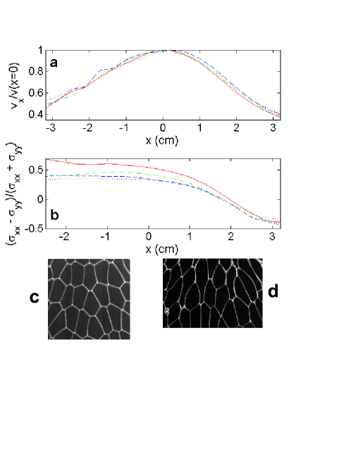
Figure 9: Effect of the surfactant. Plot of (a) the streamwise velocity component rescaled by the velocity at the middle of the contraction, $v_{x}/v(x=0)$, and (b) the normal stress difference rescaled by the total elastic stress, $(\sigma_{xx}-\sigma_{yy})/(\sigma_{xx}+\sigma_{yy})$, for four experiments: the reference experiment with a SDS solution (dotted curve), and three experiments with the SLES/CAPB/MAc mixture, with maximal velocity 0.26 (dashed curve), 0.58 (dash-dotted curve) and 1.02 cm/s (plain curve). To illustrate the change of bubble deformation, snapshots of (c) the reference experiments and (d) the fastest experiment with the SLES/CAPB/MAc mixture, taken just at the entrance of the contraction ($-3~{}\mathrm{cm}<x<-1.5~{}\mathrm{cm}$), are displayed.

5 Discussion

5.1 Interplay between elasticity, plasticity and flow

In Sec. 3 and 4, we have described separately the behavior of the velocity, elastic stress and T1 fields. We now discuss the coupling between these quantities. First, the modification of various control parameters, notably flow rate, bubble area and contraction geometry (Sec. 4.1 and 4.2), has been shown not to change the qualitative features of the flow of foam through a contraction. The effect of the foam disorder on the flow pattern remains an open question, as was pointed out by Katgert et al. (2008). We have worked with rather monodisperse foams (Fig. 1c), but our polydispersity indices are not negligible, and they vary significantly between various experiments (Tab. 1). Hence, the qualitative trends of the flow of foam through a contraction are not modified when a moderate amount of disorder is present. Consequently, the main features of the foam flow are direct consequences of the interplay of elasticity, plasticity and flow, that we can study on the reference experiment without much loss of generality.

Experiments in pure shear (Gopal and Durian, 1995) and contraction flows (Earnshaw and Wilson, 1995) have shown that the rate of plasticity is globally proportional to the rate of strain. Contrary to these studies, we have access to the local values of the deformation rate, which is displayed in Fig. 10. From these local values, we can check whether we recover a proportionality between the rate of plasticity and the deformation rate, by plotting for each box the frequency of T1s versus the norm of the deformation rate tensor, $|\bar{\bar{D}}|=\sqrt{(\bar{\bar{D}}:\bar{\bar{D}})/2}=\sqrt{(D_{xx}^{2}+2D_{xy}^{2}+D_{yy}^{2})/2}$, in Fig. 11. It shows that there is a proportionality between the rates of plasticity and deformation when these are not too large, but that there is a huge scatter at large rates of plasticity and deformation. Notably, several points at high deformation rate show very little plasticity; actually, they correspond to the small zone just at the contraction exit, where a sharp minimum of plasticity was already pinpointed in Sec. 3.3. Hence, the proportionality between rates of plasticity and deformation is not valid everywhere.

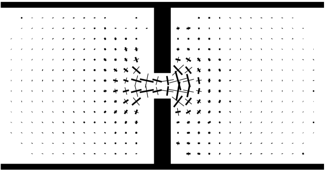
Figure 10: Deformation rate for the reference experiment. The thick (thin) lines represent the local maximal elongation (compression) rate, see Sec. 2.2.

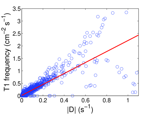
Figure 11: Frequency of T1s versus deformation rate. Each box gives one data point. The straight line is the best linear fit through all data.

We now test a more advanced coupling between elasticity, plasticity and deformation rate proposed by Marmottant et al. (2008). These authors used a plastic tensor defined as (Graner et al., 2008):

$$\bar{\bar{P}}=\frac{1}{2}f_{T1}\{(\langle\vec{r}_{d}\otimes\vec{r}_{d}\rangle-\langle\vec{r}_{a}\otimes\vec{r}_{a}\rangle)\cdot\bar{\bar{M}}^{-1}+{{}^{t}}[(\langle\vec{r}_{d}\otimes\vec{r}_{d}\rangle-\langle\vec{r}_{a}\otimes\vec{r}_{a}\rangle)\cdot\bar{\bar{M}}^{-1}]\},$$ (2)

where $\bar{\bar{M}}=\langle\vec{r}\otimes\vec{r}\rangle$ is the texture tensor (Aubouy et al., 2003), defined on the network of the vectors $\vec{r}$ linking centers of neighboring bubbles. The plastic tensor encompasses not only the frequency of T1s, but also there direction; namely, the positive (negative) eigenvalue of this (almost) traceless tensor is the preferential direction of bubble separation (attachment). As the deformation rate, we represent the plastic tensor by a pair of orthogonal lines, the thick (thin) one in the direction of the positive (negative) eigenvalue (Fig. 12). As a constitutive relation, Marmottant et al. (2008) conjectured that the plastic tensor $\bar{\bar{P}}$, the deviator of the elastic stress tensor,

$$\bar{\bar{\sigma}}_{d}=\bar{\bar{\sigma}}-\frac{1}{2}(\mathrm{tr}~{}\bar{\bar{\sigma}})\bar{\bar{I}},$$ (3)

where $\bar{\bar{I}}$ is the identity tensor, and the deformation rate $\bar{\bar{D}}$ are related through:

$$\bar{\bar{P}}=\left\{\begin{array}[]{l}\bar{\bar{0}}~{}\mathrm{if}~{}\bar{\bar{D}}:\bar{\bar{\sigma}}_{d}\leq 0\\ h(\bar{\bar{\sigma}}_{d})\dfrac{\bar{\bar{D}}:\bar{\bar{\sigma}}_{d}}{2|\bar{\bar{\sigma}}_{d}|^{2}}\bar{\bar{\sigma}}_{d}~{}\mathrm{if}~{}\bar{\bar{D}}:\bar{\bar{\sigma}}_{d}\geq 0\\ \end{array}\right.,$$ (4)

where $h$, a function varying between 0 and 1, would be the Heaviside function if the foam showed no plasticity below a yield stress $\sigma_{Y}$ and yielded abruptly at that yield stress. Notice that Eq. (4) slightly differs from the original version of Marmottant et al. (2008), where an elastic strain $\bar{\bar{U}}$ was used instead of $\bar{\bar{\sigma}}$; but since the deviators $\bar{\bar{\sigma}}_{d}$ and $\bar{\bar{U}}_{d}$ have been shown to be proportional (Asipauskas et al., 2003; Janiaud and Graner, 2005; Marmottant et al., 2008), it is equivalent to use $\bar{\bar{U}}_{d}$ or $\bar{\bar{\sigma}}_{d}$ in Eq. (4).

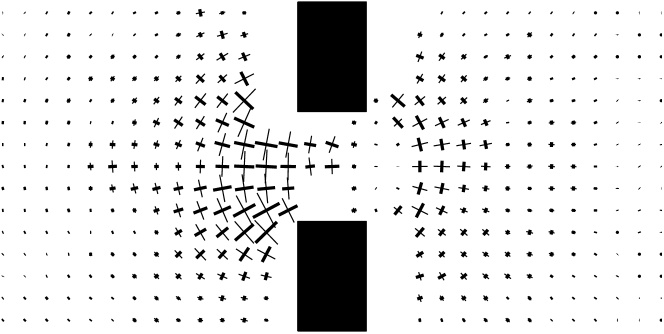
Figure 12: Plastic tensor $\bar{\bar{P}}$ for the reference experiment. The thick (thin) lines represent the direction of the eigenvector associated to the positive (negative) eigenvalues, and the line lengths are proportional to the absolute value of the eigenvalues. The points where the plastic tensor could not be reliably evaluated are left in blank.

The quantity $\bar{\bar{D}}:\bar{\bar{\sigma}}_{d}$ is proportional to $\cos 2\theta$, with $0\leq\theta\leq\pi/2$ the angle between the major axes of elastic stress and deformation rate; it is positive if $\theta\leq\pi/4$, e.g. if the two axes are aligned, and negative if $\theta\geq\pi/4$, e.g. if the two axes are proportional. If the two axes are aligned, $\bar{\bar{D}}:\bar{\bar{\sigma}}_{d}=2|\bar{\bar{D}}||\bar{\bar{\sigma}}_{d}|$, hence Eq. (4) predicts that the rate of plasticity should be proportional to the deformation rate. Since in most regions of the flow the major axes of elastic stress and deformation rate are indeed well aligned (Fig. 10 and 4a), it likely explains why there is in average a good correlation between the frequency of T1s and the deformation rate. On the contrary, the relation (4) implies that no plasticity should occur if the elastic stress and the deformation rate tend to act along opposite directions; Fig. 10 and 4a show that this is the case just at the contraction exit, and indeed this corresponds to the area with a marked minimum of plasticity. In this zone, the spanwise elongation rate serves not to trigger plastic events, but to reverse the elastic stress from streamwise to spanwise.

There is no model yet for the function $h$ entering Eq. (4), hence it is difficult to test the full relation. On the other hand, it predicts that $\bar{\bar{P}}$ should be aligned with $\bar{\bar{\sigma}}_{d}$ rather than $\bar{\bar{D}}$, which we test: we compute, for each box, the angle between the major axes of the plastic tensor and elastic stress, $\theta(P,\sigma)$, and, for comparison, the corresponding angle for the plastic tensor and deformation rate, $\theta(P,D)$, and we plot the histograms of distribution of these two angles in Fig. 13. It shows that the plastic tensor is indeed in average well aligned with the elastic stress than with the deformation rate; we have $\langle\theta(P,\sigma)\rangle=0.280~{}\mathrm{rad}=16^{\circ}$, and $\langle\theta(P,D)\rangle=0.383~{}\mathrm{rad}=22^{\circ}$. This result is a strong indication that the plasticity rate is not only related to the deformation rate, but also to the elastic stress. We do not proceed here with the discussion of the interplay of elasticity, plasticity and flow and with tests of the models. The next step would be to compare the full elastic, plastic and velocity fields in our experiments with simulations and ab initio predictions of the flow, but this is beyond the scope of this paper and will be pursued in future studies.

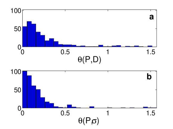
Figure 13: (a) Histogram of the angle between the major axes of the plastic tensor and elastic stress, $\theta(P,\sigma)$. (b) Histogram of the angle between the major axes of the plastic tensor and deformation rate, $\theta(P,D)$. Angles are expressed in radians and are defined in the range $[0,\pi/2]$.

At about 7 cm away from the contraction, plasticity vanishes, hence the foam behaves as a viscoelastic medium. Therefore, the velocity undershoot (reached in a zone where almost no T1s occur, see Figs. 3a and 5b) and the re-focussing of the streamlines appear as elastic effects. Indeed, the velocity undershoot is reminiscent of the negative wake phenomenon (Hassager, 1979) previously reported also in foams (Dollet and Graner, 2007), and attributed to elastic effects; at the location of the velocity undershoot, the bubbles are very elongated spanwise, and they then elastically recoil streamwise (Figs. 4a and b). Similarly, the re-focussing of streamlines may be attributed to an elastic recoil of the bubbles.

On the other hand, the velocity overshoots observed at the entrance and exit of long enough contractions (Fig. 8a) appear in yielded regions with a strong plasticity rate (Fig. 8c), hence they do not originate purely from foam elasticity. This is confirmed by the recent first observation of a velocity overshoot at the entrance of a contraction for a viscoplastic fluid, by Rabideau et al. . There does not seem to be obvious qualitative explanations for these velocity overshoots.

5.2 Interplay between surface and bulk rheologies

We have shown in Sec. 4.3 that the elastic stress depends significantly on the velocity, in the case of the SLES/CAPB/MAc mixture. This interesting observation shows that when the friction in liquid films, either between neighboring bubbles or between bubbles and walls, becomes strong enough, a dynamic parameter (here, the local value of the velocity or of the deformation rate) can influence the structure. This dynamically-induced deviation from a quasistatic foam structure (such as that fully characterized in Sec. 3, which was shown in Sec. 4.1 indeed not to depend on the flow rate) has been predicted theoretically by Kraynik and Hansen (1987) and observed in other contexts, e.g. by the deviation from the equilibrium laws governing the angles at which a film meets a wall (Drenckhan et al., 2005). Actually, this also occurs here: Fig. 9d shows that some liquid films with the SLES/CAPB/MAc mixture seem thick, seen from above. This apparent increased thickness is nothing but the larger horizontal section of the films that exhibit a strong curvature across the gap between the two plates; this is also related to deviations from the equilibrium laws, because a liquid film between two bubbles at equilibrium is straight and perpendicular to the walls.

It would be interesting then to compare our experimental snapshots with shape predictions from the viscous froth model (Kern et al., 2004), which is already used to study the morphology of single films and bubbles (Grassia et al., 2008; Cox et al., 2009) under the effect of friction acting on Plateau borders, where a liquid film meets a wall. However, we have here two sources of friction: between bubbles and walls, or between neighboring bubbles. When the latter dominates, which is usually the case in 3D foams, it has been observed that the yield strain, i.e. the applied strain at the onset of plasticity, is an increasing function of the applied strain rate (Rouyer et al., 2003). This was indeed interpreted as a consequence of the internal viscous stresses. Work is in progress to study the influence of one or the other on dynamical modification of the foam structure, in simpler geometries.

Finally, let us stress that such a variation of the elastic stress is a priori possible also for the SDS solution. However, its surface viscoelasticity is two orders of magnitude lower than that of the SLES/CAPB/MAc mixture, hence deviations from the quasistatic regime are not expected under velocities of order 1 m/s, which is beyond the range of flow rates that we can produce with our setup.

6 Conclusions

We have experimentally investigated the two-dimensional flow of foam through a contraction. Thanks to image analysis, we could extract a rather complete information on the foam behavior, in terms of elastic stresses, plastic events, and flow. The flow exhibits a strong fore-aft asymmetry (with respect to the contraction center) and some striking features, such as a velocity undershoot at the contraction exit. The qualitative features of the flow are rather insensitive to control parameters such as the bubble size and contraction width and length, as well as the flow rate, provided it is low enough (quasistatic regime). Conversely, as friction within the liquid films becomes significant, for instance using surfactants with a strong surface viscoelasticity, the elastic stresses show a strong dependence on the flow velocity.

By comparing elastic and plastic local descriptors of the foam and its flow profile, we have been able to show that there is an essential coupling between elasticity, plasticity and flow. Notably, there is not everywhere a proportionality between the rates of plasticity and deformation, and the relative orientation of elastic stresses and deformation rate plays a fundamental role, which encourages to further develop and test tensorial viscoelastoplastic models for foam rheology. As another perspective of this work, the interesting coupling between surface and bulk rheologies deserves to be further investigated and understood, first in simple geometries (plug flow).

References

- Abdali et al. (1992) S. S. Abdali, E. Mitsoulis, and N. C. Markatos. Entry and exit flows of bingham fluids. J. Rheol., 36:389–407, 1992.
- Asipauskas et al. (2003) M. Asipauskas, M. Aubouy, J. A. Glazier, F. Graner, and Y. Jiang. A texture tensor to quantify deformations: the example of two-dimensional flowing foams. Granular Matter, 5:71–74, 2003.
- Aubouy et al. (2003) M. Aubouy, Y. Jiang, J. A. Glazier, and F. Graner. A texture tensor to quantify deformations. Granular Matter, 5:67–70, 2003.
- Batchelor (1970) G. K. Batchelor. The stress system in a suspension of force-free particules. J. Fluid Mech., 41:545–570, 1970.
- Bénito et al. (2008) S. Bénito, C. H. Bruneau, T. Colin, C. Gay, and F. Molino. An elasto-visco-plastic model for immortal foams or emulsions. Eur. Phys. J. E, 25:225–251, 2008.
- Bertho et al. (2006) Y. Bertho, C. Becco, and N. Vandewalle. Dense bubble flow in a silo: an unusual flow of a dispersed medium. Phys. Rev. E, 73:056309, 2006.
- Cantat and Pitois (2006) I. Cantat and O. Pitois. Stokes experiment in a liquid foam. Phys. Fluids, 18:083302, 2006.
- Cantat et al. (2006) I. Cantat, C. Poloni, and R. Delannay. Experimental evidence of flow destabilization in a two-dimensional bidisperse foam. Phys. Rev. E, 73:011505, 2006.
- Cheddadi et al. (2008) I. Cheddadi, P. Saramito, C. Raufaste, P. Marmottant, and F. Graner. Numerical modelling of foam couette flows. Eur. Phys. J. E, 27:123–133, 2008.
- Cox et al. (2009) S. J. Cox, D. Weaire, and G. Mishuris. The viscous froth model: steady states and the high-velocity limit. Proc. Roy. Soc. A, 465:2391–2405, 2009.
- Debrégeas et al. (2001) G. Debrégeas, H. Tabuteau, and J.-M. di Meglio. Deformation and flow of a two-dimensional foam under continuous shear. Phys. Rev. Lett., 87:178305, 2001.
- Denkov et al. (2005) N. D. Denkov, V. Subramanian, D. Gurovich, and A. Lips. Wall slip and viscous dissipation in sheared foams: Effect of surface mobility. Colloids Surf. A, 263:129–145, 2005.
- Denkov et al. (2009) N. D. Denkov, S. Tcholakova, K. Golemanov, and A. Lips. Jamming in sheared foams and emulsions, explained by critical instability of the films between neighboring bubbles and drops. Phys. Rev. Lett., 103:118302, 2009.
- Dennin (2004) M. Dennin. Statistics of bubble rearrangements in a slowly sheared two-dimensional foam. Phys. Rev. E, 70:041406, 2004.
- Dollet and Graner (2007) B. Dollet and F. Graner. Two-dimensional flow of foam around a circular obstacle: local measurements of elasticity, plasticity and flow. J. Fluid Mech., 585:181–211, 2007.
- Dollet et al. (2005) B. Dollet, M. Aubouy, and F. Graner. Anti-inertial lift in foams: A signature of the elasticity of complex fluids. Phys. Rev. Lett., 95:168303, 2005.
- Dollet et al. (2006) B. Dollet, M. Durth, and F. Graner. Flow of foam past an elliptical obstacle. Phys. Rev. E, 73:061404, 2006.
- Drenckhan et al. (2005) W. Drenckhan, S. J. Cox, G. Delaney, H. Holste, D. Weaire, and N. Kern. Rheology of ordered foams—on the way to discrete microfluidics. Colloids Surf. A, 263:52–64, 2005.
- Durian et al. (1991) D. J. Durian, D. A. Weitz, and D. J. Pine. Multiple light-scattering probes of foam structure and dynamics. Science, 252:686, 1991.
- Earnshaw and Wilson (1995) J. C. Earnshaw and M. Wilson. Strain-induced dynamics of flowing foam: an experimental study. J. Phys. Condens. Matter, 7:L49–L53, 1995.
- Earnshaw and Wilson (1996) J. C. Earnshaw and M. Wilson. A diffusing wave spectroscopy study of constrictive flow of foam. J. Phys. II France, 6:713–722, 1996.
- Golemanov et al. (2008) K. Golemanov, N. D. Denkov, S. Tcholakova, M. Vethamuthu, and A. Lips. Surfactant mixtures for control of bubble surface mobility in foam studies. Langmuir, 24:9956–9961, 2008.
- Gopal and Durian (1995) A. D. Gopal and D. J. Durian. Nonlinear bubble dynamics in a slowly driven foam. Phys. Rev. Lett., 75:2610–2613, 1995.
- Graner et al. (2008) F. Graner, B. Dollet, C. Raufaste, and P. Marmottant. Discrete rearranging disordered patterns, part i: Robust statistical tools in two or three dimensions. Eur. Phys. J. E, 25:349–369, 2008.
- Grassia et al. (2008) P. Grassia, G. Montes-Atenas, L. Lue, and T. E. Green. A foam film propagating in a confined geometry: Analysis via the viscous froth model. Eur. Phys. J. E, 25:39–49, 2008.
- Hassager (1979) O. Hassager. Negative wake behind bubbles in non-newtonian fluids. Nature, 279:402–403, 1979.
- Höhler and Cohen-Addad (2005) R. Höhler and S. Cohen-Addad. Rheology of liquid foams. J. Phys. Condens. Matter, 17:R1041–R1069, 2005.
- Höhler et al. (1997) R. Höhler, S. Cohen-Addad, and H. Hoballah. Periodic nonlinear bubble motion in aqueous foam under oscillating shear strain. Phys. Rev. Lett., 79:1154–1157, 1997.
- Janiaud and Graner (2005) É. Janiaud and F. Graner. Foam in a two-dimensional couette shear: a local measurement of bubble deformation. J. Fluid Mech., 532:243–267, 2005.
- Janiaud et al. (2006) É. Janiaud, D. Weaire, and S. Hutzler. Two-dimensional foam rheology with viscous drag. Phys. Rev. Lett., 97:038302, 2006.
- Jay et al. (2002) P. Jay, A. Magnin, and J. M. Piau. Numerical simulation of viscoplastic fluid flows through an axisymmetric contraction. J. Fluids Eng., 124:700–705, 2002.
- Katgert et al. (2008) G. Katgert, M. E. Möbius, and M. van Hecke. Rate dependence and role of disorder in linearly sheared two-dimensional foams. Phys. Rev. Lett., 101:058301, 2008.
- Katgert et al. (2009) G. Katgert, A. Latka, M. E. Möbius, and M. van Hecke. Flow in linearly sheared two-dimensional foams: From bubble to bulk scale. Phys. Rev. E, 79:066318, 2009.
- Kern et al. (2004) N. Kern, D. Weaire, A. Martin, S. Hutzler, and S. J. Cox. Two-dimensional viscous froth model for foam dynamics. Phys. Rev. E, 70:041411, 2004.
- Kraynik and Hansen (1987) A. M. Kraynik and M. G. Hansen. Foam rheology: A model of viscous phenomena. J. Rheol., 31:175–205, 1987.
- Lambert et al. (2007) J. Lambert, I. Cantat, R. Delannay, R. Mokso, P. Cloetens, J. A. Glazier, and F. Graner. Experimental growth law for bubbles in a moderately “wet” 3D liquid foam. Phys. Rev. Lett., 99:058304, 2007.
- Langlois et al. (2008) V. Langlois, S. Hutzler, and D. Weaire. Rheological properties of the soft-disk model of two-dimensional foams. Phys. Rev. E, 78:021401, 2008.
- Marmottant et al. (2008) P. Marmottant, C. Raufaste, and F. Graner. Discrete rearranging disordered patterns, part ii: 2d plasticity, elasticity and flow of a foam. Eur. Phys. J. E, 25:371–384, 2008.
- (39) B. D. Rabideau, P. Moucheront, F. Bertrand, S. Rodts, N. Roussel, C. Lanos, and P. Coussot. The extrusion of a model yield stress fluid imaged by mri velocimetry. J. Non-Newtonian Fluid Mech. submitted.
- Rouyer et al. (2003) F. Rouyer, S. Cohen-Addad, M. Vignes-Adler, and R. Höhler. Dynamics of yielding observed in a three-simensional aqueous dry foam. Phys. Rev. E, 267:021405, 2003.
- Russev et al. (2008) S. C. Russev, N. Alexandrov, K. G. Marinova, K. D. Danov, N. D. Denkov, L. Lyutov, V. Vulchev, and C. Bilke-Krause. Instruments and methods for surface dilatational rheology measurements. Rev. Sci. Instr., 79:104102, 2008.
- Saramito (2007) P. Saramito. A new constitutive equation for elastoviscoplastic fluid flows. J. Non-Newtonian Fluid Mech., 145:1–14, 2007.
- Saramito (2009) P. Saramito. A new elastoviscoplastic model based on the herschel- bulkley viscoplastic model. J. Non-Newtonian Fluid Mech., 158:154–161, 2009.
- Vaz and Cox (2005) M. F. Vaz and S. J. Cox. Two-bubble instabilities in quasi-two-dimensional foams. Phil. Mag. Lett., 85:415–425, 2005.
- Vera et al. (2001) M. U. Vera, A. Saint-Jalmes, and D. J. Durian. Scattering optics of foam. Appl. Opt., 40:4210–4214, 2001.
- Wang et al. (2006) Y. Wang, K. Krishan, and M. Dennin. Impact of boundaries on velocity profiles in bubble rafts. Phys. Rev. E, 73:031401, 2006.
- Weaire and Hutzler (1999) D. Weaire and S. Hutzler. The Physics of Foams. Oxford University Press, 1999.