Abstract

We present a model of electroweak symmetry breaking in a warped extra dimension where electroweak symmetry is broken at the UV (or Planck) scale. An underlying conformal symmetry is broken at the IR (or TeV) scale generating masses for the electroweak gauge bosons without invoking a Higgs mechanism. By the AdS/CFT correspondence the $W,Z$ bosons are identified as composite states of a strongly-coupled gauge theory, suggesting that electroweak symmetry breaking is an emergent phenomenon at the IR scale. The model satisfies electroweak precision tests with reasonable fits to the $S$ and $T$ parameter. In particular the $T$ parameter is sufficiently suppressed since the model naturally admits a custodial $SU(2)$ symmetry. The composite nature of the $W,Z$-bosons provide a novel possibility of unitarizing $WW$ scattering via form factor suppression. Constraints from LEP and the Tevatron as well as discovery opportunities at the LHC are discussed for these composite electroweak gauge bosons.

1 Introduction

A major goal of the Large Hadron Collider (LHC) is to unveil the origin of electroweak symmetry breaking (EWSB). In the Standard Model (SM) the Higgs mechanism provides a particularly attractive way to break electroweak symmetry and generate mass. It is most simply implemented by introducing the Higgs boson, a scalar field that spontaneously breaks the electroweak symmetry by obtaining a vacuum expectation value (VEV). If the Higgs boson is an elementary scalar field then its mass can be stabilized by low-energy supersymmetry. In this case supersymmetry breaking triggers the breaking of electroweak symmetry. Alternatively the Higgs boson may be composite and therefore can be stabilized with strong dynamics at the TeV scale [1]. A composite Higgs boson model was recently constructed using the holographic dual of a warped dimension [2]. But the presence of a Higgs boson is not obligatory. As is well-known by analogy with QCD, electroweak symmetry can also be broken by condensates in technicolor. In fact, via the AdS/CFT correspondence, a technicolor-like Higgsless model can be constructed in a warped extra dimension providing a more recent incarnation of this idea [3]. Nevertheless the underlying feature of all these models is that electroweak symmetry is broken at the electroweak scale where, in particular, the Standard Model gauge fields and fermions receive a mass by coupling to an external Higgs sector. To generate (not just stabilize) the TeV mass scale or gauge hierarchy in a natural way via dimensional transmutation, it seems inevitable to have strong dynamics in this external sector (whether it be associated with electroweak or supersymmetry breaking), together with the Standard Model gauge fields and fermions which do not directly partake in the underlying dynamics.

Yet there is another possibility for mass generation. Just like the hadron mass spectrum in QCD, there is no need to invoke the Higgs mechanism to generate a mass. Instead the fermions and $W,Z$-bosons could be composite states which directly obtain a mass from the underlying confining strong dynamics. This idea is not new [4], since QCD contains states which mimic the electroweak gauge bosons. Specifically it was noticed that low-energy QCD can be interpreted as a spontaneously broken gauge theory, where the SU(2) isospin triplet $\rho$ meson is the massive gauge field of a hidden local symmetry [5]. Interestingly this interpretation can effectively explain $\rho$-coupling universality, $\rho$-meson dominance, and the high-energy $\pi$-$\pi$ scattering cross section. This bears some resemblance with electroweak symmetry suggesting that the $W,Z$-bosons might be composite. Furthermore, unlike global symmetries, gauge symmetries do not lead to new conserved charges and merely remove the redundancy in our description of massless spin-1 particles with spacetime vector fields. This has led to the suggestion that gauge symmetries are not fundamental [6]. In fact this is supported by duality in four-dimensional (4D) supersymmetric theories which imply that gauge symmetries in the SM or even general relativity could be long-distance artifacts [7]. So the idea that electroweak gauge bosons are composite represents an intriguing although relatively unexplored possibility.

In this paper we examine this possibility by constructing an EWSB model with composite $W,Z$ bosons. Since the underlying theory is inherently strongly-coupled we use the AdS/CFT correspondence [8, 9] to construct a calculable five-dimensional (5D) model using a warped fifth dimension [10]. The electroweak symmetry will be assumed to be preserved on the IR brane and the bulk, while it will be broken on the UV brane. Hence in this model the IR brane is only used to break conformal symmetry and generate massive states. This is opposite from the original Randall-Sundrum model and all other warped models where EWSB is assumed to occur on the IR brane. This implies that in our model electroweak gauge symmetry is not a fundamental symmetry and merely emerges at the IR scale when the conformal symmetry is broken. Moreover even though our model is effectively Higgsless at low energies because EWSB occurs on the UV brane and the Higgs sector decouples, it still differs from the usual technicolor-like Higgsless model [3] where EWSB occurs at the IR scale and the $W,Z$-boson are elementary fields.

Brane kinetic terms are a crucial feature of our model. In order to identify the lightest Kaluza-Klein (KK) states with composite $W,Z$ bosons they are introduced to separate the lowest-lying KK mode from the rest of the KK tower. This guarantees that the heavier KK resonances of the $W,Z$ bosons are sufficiently heavy to evade direct experimental bounds. This leads to $W$ and $Z$ boson profiles that are effectively localized near the IR brane, rendering them composite states of the dual 4D theory. While the main focus of this work will be on the gauge boson sector we will make simplifying assumptions regarding the fermion sector. Since electroweak symmetry is broken on the UV brane, fermions must at least couple to the UV brane and have universal profiles in the bulk to ensure gauge coupling universality. This will be left for future work and for simplicity we will assume the fermions are localized on the IR brane.

The idea of composite weak gauge bosons has been previously explored in the literature [4] where attempts were made to construct the underlying preon models based on asymptotically-free QCD. Unlike these earlier attempts the AdS/CFT dictionary relates our composite gauge boson model to a dual 4D conformal field theory at large ‘t Hooft coupling. In addition the weakly-coupled 5D gravity dual improves calculability allowing a more quantitative analysis of the composite model. Consequently, a precision electroweak analysis can be performed leading to reasonable agreement with the $S,T$ parameters. In particular, the $T$ parameter is sufficiently suppressed due to a custodial SU(2) symmetry that naturally occurs in the model. Since the gauge bosons are composite there are also various interesting phenomenological aspects to study. In fact due to the strong coupling the underlying composite nature of the gauge bosons is much less partonic at moderate Bjorken $x$ compared to QCD hadrons. In particular the composite nature of the $W,Z$ boson provides a novel unitarization mechanism for $WW$ scattering based on form factor suppression, and suggests that deviations in the scattering amplitude may be measurable, giving rise to a distinctive signal at the LHC.

The organization of this paper is as follows. In Section 2 we present an overview of the model, outlining our various assumptions before presenting the full details of the 5D model in a warped dimension. The electroweak precision analysis is presented in Section 3 where it is shown how the model naturally admits a custodial SU(2) symmetry. The $S$ and $T$ parameter are both shown to be consistent with electroweak precision tests. Section 4 is devoted to a preliminary study on $WW$ scattering and unitarity. Various constraints and signatures of composite weak gauge bosons at LEP, Tevatron, and the LHC are discussed in Section 5. Finally in Appendix A we present an alternative derivation of how brane kinetic terms give rise to a light KK mode, while in Appendix B we present a form factor computation using the overlap integral.

2 Emergent EWSB

2.1 The 5D Model

We begin by defining our EWSB model using the Randall-Sundrum framework [10]. Consider a slice of AdS₅ with 5D metric

$$ds^{2}=\frac{1}{(kz)^{2}}(\eta_{\mu\nu}dx^{\mu}dx^{\nu}+dz^{2})\equiv g_{MN}dx^{M}dx^{N}~{},$$ (1)

where $k$ is the AdS curvature scale. The 5D spacetime indices are written as $M=(\mu,5)$, with $\mu=0,1,2,3$, and $\eta_{\mu\nu}={\rm diag}(-+++)$ is the Minkowski metric. The fifth dimension $z$ is compactified on a $Z_{2}$ orbifold, with a UV (IR) brane located at the fixed point $z^{*}=z_{UV}(z_{IR})$. The $z$ coordinate is related to the 4D energy scale, and the scale of the UV (IR) brane is chosen to be $z_{UV}=k^{-1},(z_{IR}={\cal O}({\rm TeV}^{-1}))$ respectively, where $k\simeq M_{P}=2.4\times 10^{18}$ GeV is the reduced Planck scale.

The 5D bulk is assumed to have an electroweak symmetry, $SU(2)_{L}\times U(1)_{Y}$, while on the boundaries the electroweak symmetry is preserved on the IR brane but broken on the UV brane. This is to ensure that the $W,Z$ bosons are identified with the lowest-lying KK modes peaking towards the IR brane, so that by the AdS/CFT correspondence they are interpreted as composite states. On the UV brane the symmetry is broken by imposing Dirichlet boundary conditions that realizes the SM symmetry breaking pattern $SU(2)_{L}\times U(1)_{Y}\rightarrow U(1)_{Q}$. As pointed out in [3] EWSB via Dirichlet boundary conditions can be more naturally understood as the limit of a Higgs mechanism on the boundary with a very large VEV. Since the breaking is on the UV brane, the Higgs sector decouples and the model is effectively Higgsless at low energies. The unbroken electromagnetic group $U(1)_{Q}$ on the UV brane leads to a massless photon. In addition, even though the strong force is irrelevant for our discussion, there are massless gluons from the unbroken $SU(3)$ color symmetry. So in our setup, the massive $W,Z$ gauge fields are mostly composite, while the massless gauge fields are mostly elementary.

There is an immediate problem with identifying the lowest-lying KK states with the $W,Z$ bosons. Since in the warped dimension the KK modes are essentially evenly spaced, the next-heaviest KK states will have masses at approximately 200 GeV. This obviously contradicts direct searches and electroweak precision data that require additional electroweak gauge bosons $(i.e.\,W^{\prime},Z^{\prime})$ to be heavier than about $1\,\rm TeV$ [11]. Hence to obtain a desirable mass spectrum we will introduce brane-localized kinetic terms [12, 13]. We will see that this leads to very light lowest-lying KK modes for the $W,Z$ bosons, while the remaining heavier KK modes of the $W,Z$-boson and photon will appear at the TeV scale. Brane kinetic terms will be added on both branes consistent with the brane symmetry. This includes mass-dimension $-1$ brane kinetic term coefficients $\zeta_{Q}$ for $U(1)_{Q}$ on the UV brane, and $\zeta_{L},\zeta_{Y}$ for $SU(2)_{L}$ and $U(1)_{Y}$ on the IR brane, respectively. Thus the 5D action of our model is given by

$$S=\int d^{4}x\,dz\sqrt{-g}\left[-\frac{1}{4}(F^{La}_{MN})^{2}-\frac{1}{4}(F^{Y}_{MN})^{2}-\frac{1}{2}(kz)\delta{(z-z_{UV})}\frac{\zeta_{Q}}{g_{Y5}^{2}+g^{2}_{L5}}(g_{Y5}F^{L3}_{\mu\nu}+g_{L5}F^{Y}_{\mu\nu})^{2}\right.$$

$$\left.-\frac{1}{2}(kz)\delta{(z-z_{IR})}\left(\zeta_{L}(F^{La}_{\mu\nu})^{2}+\zeta_{Y}(F^{Y}_{\mu\nu})^{2}\right)\right],$$ (2)

where the 5D field strengths $F^{L}_{MN},F^{Y}_{MN}$ with associated gauge fields $A^{L}_{M},B_{M}$, and 5D gauge couplings $g_{L5},g_{Y5}$, are for $SU(2)_{L},U(1)_{Y}$, respectively. Since only the UV boundary is Higgsed, the fifth components of the gauge fields are unphysical [14]. This ensures that our model contains no $A_{5}$-like holographic Higgs bosons.

Note that the brane kinetic terms in (2) are crucial ingredients in our model. They are always allowed on the branes at tree level by the breaking of 5D Poincare symmetry. But more importantly in any 5D theory with bulk gauge fields, as well as charged bulk matter subject to orbifold boundary conditions [12] or confined to the branes [15], the divergent radiative corrections to the gauge propagator requires that brane kinetic terms be included as counterterms. Therefore from the effective field theory perspective the coefficients of the brane kinetic terms are free parameters of the theory with their exact values depending on the UV completion. Although naive dimensional analysis (NDA) estimates the size of the coefficients to be of order the compactification scale of the fifth dimension [16, 17, 18], large brane kinetic terms are perturbatively consistent [19]. Thus, just like previous analyses in [17, 13], we will assume the brane kinetic term coefficients to be free parameters that are fixed by experimental data, and do not constrain them to be of their NDA size.

2.1.1 The gauge boson mass spectrum

The boundary conditions that realize the symmetry breaking pattern and include the brane kinetic terms are

$$z=z_{UV}:\left\{\begin{array}[]{l}\hbox{$\partial_{z}(g_{Y5}A^{L3}_{\mu}+g_{L5}B_{\mu})+\zeta_{Q}kz_{IR}\Box(g_{Y5}A^{L3}_{\mu}+g_{L5}B_{\mu})=0,$}\\ \hbox{$g_{L5}A^{L3}_{\mu}-g_{Y5}B_{\mu}=0,$}\\ \hbox{$A^{L1,2}_{\mu}=0,$}\end{array}\right.$$ (6)

$$z=z_{IR}:\left\{\begin{array}[]{l}\hbox{$\partial_{z}A_{\mu}^{La}-\zeta_{L}kz_{IR}\Box A_{\mu}^{La}=0,$}\\ \hbox{$\partial_{z}B_{\mu}-\zeta_{Y}kz_{IR}\Box B_{\mu}=0,$}\end{array}\right.$$ (9)

where $\Box=\eta_{\mu\nu}\partial^{\mu}\partial^{\nu}$ is the 4D Laplacian. Imposing these boundary conditions on the bulk solutions will lead to the mass spectrum and is similar to that performed in Refs. [17, 20, 13]. Gauge fields which are mixed by the boundary conditions share the same KK mass spectrum (although with a different 5D profile for the same KK mode). In particular this is the KK tower containing both $A_{\mu}^{L3}$ and $B_{\mu}$. When $B_{\mu}$ is dominant, it is identified as the KK photon tower, while when $A_{\mu}^{L3}$ is dominant, it is identified as the KK $Z$-boson tower. For the other tower, $A_{\mu}^{L\pm}$ is identified as the KK $W$-boson tower where $A_{\mu}^{L\pm}$ denotes the linear combination $\frac{1}{\sqrt{2}}(A_{\mu}^{L1}\mp iA_{\mu}^{L2}$). The KK decomposition is therefore given by

$$A_{\mu}^{L3}(x,z) = f_{0}^{L3}(z)\gamma_{\mu}(x)+\displaystyle\sum_{n=1}^{\infty}f^{L3}_{n}(z)Z_{\mu}^{(n)}(x),$$ (10)

$$B_{\mu}(x,z) = f^{B}_{0}(z)\gamma_{\mu}(x)+\displaystyle\sum_{n=1}^{\infty}f^{B}_{n}(z)Z_{\mu}^{(n)}(x),$$ (11)

$$A_{\mu}^{L\pm}(x,z) = \displaystyle\sum_{n=1}^{\infty}f^{L\pm}_{n}(z)W_{\mu}^{(n)\pm}(x).$$ (12)

We have separated out the photon $\gamma_{\mu}$ in the decomposition of $A_{\mu}^{L3},B_{\mu}$ since later we will show that there is a massless flat zero mode in this KK tower. Substituting these decompositions into the boundary conditions (6) and (9), leads to the explicit boundary conditions for the 5D profile functions:

$$z=z_{UV}:\left\{\begin{array}[]{l}\hbox{$\partial_{z}(g_{Y5}f^{L3}_{n}(z)+g_{L5}f^{B}_{n}(z))+\zeta_{Q}\,kz_{IR}\,m_{Z_{n}}^{2}(g_{Y5}f^{L3}_{n}(z)+g_{L5}f^{B}_{n}(z))=0,$}\\ \hbox{$g_{L5}f^{L3}_{n}(z)-g_{Y5}f^{B}_{n}(z)=0,$}\\ \hbox{$f^{L\pm}_{n}(z)=0,$}\\ \end{array}\right.$$ (16)

$$z=z_{IR}:\left\{\begin{array}[]{l}\hbox{$\partial_{z}(f^{L3}_{n}(z))-\zeta_{L}\,kz_{IR}\,m_{Z_{n}}^{2}f^{L3}_{n}(z)=0,$}\\ \hbox{$\partial_{z}(f^{L\pm}_{n}(z))-\zeta_{L}\,kz_{IR}\,m_{W_{n}}^{2}f^{L\pm}_{n}(z)=0,$}\\ \hbox{$\partial_{z}(f^{B}_{n}(z))-\zeta_{Y}\,kz_{IR}\,m_{Z_{n}}^{2}f^{B}_{n}(z)=0,$}\end{array}\right.$$ (20)

where $\Box Z_{\mu}^{(n)}(x)=m_{Z_{n}}^{2}Z_{\mu}^{(n)}(x)$ and $\Box W_{\mu}^{(n)\pm}(x)=m_{W_{n}}^{2}W_{\mu}^{(n)\pm}(x)$. The equation of motion for the gauge field 5D profiles $f_{n}(z)$ is

$$\left(\partial_{z}^{2}-\frac{1}{z}\partial_{z}+m_{n}^{2}\right)f_{n}=0.$$ (21)

The general solution for the massless zero mode ($m_{0}=0$) is given by

$$f_{0}(z)=N_{0}+b_{0}z^{2},$$ (22)

while for the massive mode the general solution is

$$f_{n}(z)=N_{n}z(J_{1}(m_{n}z)+b_{n}Y_{1}(m_{n}z)),$$ (23)

where the coefficients $N_{n},b_{n}$ are fixed by the boundary conditions and normalization condition.

We first check whether the zero mode solution (22) satisfies the boundary conditions (16) and (20). We find that no zero mode exists for $f_{0}^{L\pm}$, while for $f_{0}^{L3},f_{0}^{B}$ there is a constant zero mode solution

$$f^{L3}_{0}(z)=\frac{N_{0}}{g_{L5}};\qquad f^{B}_{0}(z)=\frac{N_{0}}{g_{Y5}},$$ (24)

where $N_{0}$ is fixed by the normalization condition. The photon wavefunction is $f_{\gamma}(z)=\sqrt{(f_{0}^{L3})^{2}+(f_{0}^{B})^{2}}$.

Next we check the massive mode solutions, $f^{L\pm}_{n}(z)$, $f^{L3}_{n}(z)$ and $f^{B}_{n}(z)$. The boundary conditions determine $m_{n}$ and $b_{n}$, while the overall prefactors $N_{n}$ are fixed by the normalization condition (which we will do later). To simplify the expressions, it is also useful to define new variables: $\beta_{5}\equiv g_{L5}/g_{Y5},x_{n}\equiv m_{n}z_{IR},t\equiv z_{UV}/z_{IR}$. Due to the nontrivial boundary conditions and Bessel function properties, numerical techniques are normally required to solve fo $m_{n}$ and $b_{n}$. However, since we expect there are ultra-light lowest-lying KK modes satisfying $m_{1}z_{UV}\ll m_{1}z_{IR}\ll 1$, corresponding to the $W/Z$-bosons, we can use a small argument expansion for the Bessel functions to obtain a good analytic approximation for the $W/Z$-boson masses. This also provides an extra check for the existence of light lowest-lying KK modes.

Consider first the analytic solution for the $W$-boson tower wavefunctions ($f^{L\pm}_{n}$). The coefficients $b_{n}^{L\pm}$ are given by

$$b_{n}^{L\pm}=-\frac{J_{1}(x_{n}t)}{Y_{1}(x_{n}t)},$$ (25)

and the KK masses are the zeroes of the algebraic equation

$$Y_{1}(x_{n}t)[J_{0}(x_{n})-k\zeta_{L}x_{n}J_{1}(x_{n})]-J_{1}(x_{n}t)[Y_{0}(x_{n})-k\zeta_{L}x_{n}Y_{1}(x_{n})]=0.$$ (26)

The $W$-boson is identified with the lowest-lying KK mode and an approximate expression is given by

$$m_{W}\simeq\sqrt{\frac{2}{\zeta_{L}k}}\,z_{IR}^{-1}.$$ (27)

Therefore to obtain the observed value $m_{W}=80.4$ GeV, assuming $z_{IR}^{-1}=1$ TeV, we need $\zeta_{L}k\simeq 310$. Using $b_{1}^{L\pm}\simeq(\pi t^{2})/(2k\zeta_{L})$ the $W$-boson 5D profile to leading order becomes

$${\tilde{f}}_{W}(z)=\frac{1}{2}m_{W}z^{2}.$$ (28)

where $f_{W}(z)\equiv f_{1}^{L\pm}(z)$ and we write $f_{W}(z)\equiv N_{W}{\tilde{f}}_{W}(z)$ with $N_{W}$ a normalization constant. Thus, with respect to a flat metric the profile is peaked towards the IR brane.

Due to the nontrivial boundary conditions, the solution for the $Z$-boson tower is not as simple. The expressions for the wavefunction coefficients are

$$b_{n}^{L3,B} = \frac{\zeta_{L,Y}kx_{n}J_{1}(x_{n})-J_{0}(x_{n})}{Y_{0}(x_{n})-\zeta_{L,Y}kx_{n}Y_{1}(x_{n})}\stackrel{{\scriptstyle n=1}}{{\simeq}}\frac{(\frac{1}{2}\zeta_{L,Y}kx_{1}^{2}-1)\frac{\pi}{2}}{\log(\frac{x_{1}}{2})+\gamma_{E}+\zeta_{L,Y}k},$$ (29)

$$\frac{N_{n}^{B}}{N_{n}^{L3}} = \beta_{5}\frac{J_{1}(x_{n}t)+b_{n}^{L3}Y_{1}(x_{n}t)}{J_{1}(x_{n}t)+b_{n}^{B}Y_{1}(x_{n}t)}\stackrel{{\scriptstyle n=1}}{{\simeq}}\beta_{5}\frac{b_{n}^{L3}}{b_{n}^{B}},$$ (30)

where $\gamma_{E}\simeq 0.577$ is the Euler-Macheroni constant. Substituting the 5D profiles into the first line of the boundary condition (16), gives the $Z$-boson mass equation:

$$J_{0}(x_{n}t)+b_{n}^{L3}Y_{0}(x_{n}t)+\beta_{5}\frac{N_{n}^{B}}{N_{n}^{L3}}(J_{0}(x_{n}t)+b_{n}^{B}Y_{0}(x_{n}t))+\zeta_{Q}k(1+\beta_{5}^{2})x_{n}t(J_{1}(x_{n}t)+b_{n}^{L3}Y_{1}(x_{n}t))=0.$$ (31)

Using the expressions (29) and (30), an approximate solution of (31) can be obtained in the limit of vanishing $\zeta_{Y}$ and large $\zeta_{Q}$ (i.e. $\zeta_{Q}\gg\log t$), with $\beta_{5}\sim{\cal O}(1)$ (as we will see this limit also helps to obtain a good fit to the $T$ parameter). This leads to the $Z$-boson mass:

$$m_{Z}\simeq\sqrt{\frac{2}{\zeta_{L}k}+\frac{2}{\zeta_{Q}k(1+\beta_{5}^{2})}}\,z_{IR}^{-1}~{}.$$ (32)

Assuming $z_{IR}^{-1}=1$ TeV, the observed $Z$-boson mass, $m_{Z}=91.2$ GeV, is obtained for $\zeta_{Q}k\simeq 500$. Note that in the large $\zeta_{Q}$ or large $\beta_{5}$ limit, $m_{Z}=m_{W}$, suggesting that there is a custodial symmetry in our model, as we will show later. An approximate analytic expression for the 5D $Z$-boson profile can also be obtained in the above limit from $f_{1}^{L3}$ and $f_{1}^{B}$, giving rise to

$${\tilde{f}}^{L3}_{1}(z) = \frac{1}{2}m_{Z}z^{2}-\frac{m_{Z}^{-1}}{\zeta_{Q}k(1+\beta_{5}^{2})},$$ (33)

$${\tilde{f}}^{B}_{1}(z) = -\frac{\beta_{5}\log(m_{Z}z_{IR})}{2\zeta_{Q}k(1+\beta_{5}^{2})}m_{Z}z^{2}-\frac{\beta_{5}m_{Z}^{-1}}{\zeta_{Q}k(1+\beta_{5}^{2})},$$ (34)

where $f_{1}^{L3,B}\equiv N_{Z}{\tilde{f}}_{1}^{L3,B}$ and $N_{Z}$ is a normalization constant. The $Z$-boson profile is then given by $f_{Z}(z)=\sqrt{(f_{1}^{L3})^{2}+(f_{1}^{B})^{2}}$ and the $W/Z$-boson profiles are plotted in Figure 1. Thus we again see that with respect to a flat metric, just like the $W$-boson, the $Z$-boson is localized near the IR brane.

Figure 1: The $W$-boson (solid) and $Z$-boson (dashed) profiles in units of $\sqrt{k}$.

It is important to note that the bulk profiles (28), (33), and (34), plotted in Figure 1 do not depict the complete localization information. Recall that the profile density $|f(z)|^{2}$ represents the probability of finding a particular mode in the AdS slice (including the branes). The canonical normalization of the profile ensures a unit probability of locating the mode somewhere in the AdS slice. However the bulk profiles depicted in Figure 1 do not give rise to a unit probability distribution, in fact they only contribute a small fraction to the whole normalization. This is because the contributions from the boundary kinetic terms are not shown. They actually give rise to a large contribution to the normalization which together with the bulk contribution leads to a unit probability distribution.

Since the boundary kinetic terms are given in terms of a singular $\delta$-function their contribution cannot be depicted in Figure 1. This is related to the assumption that the branes are infinitely thin, which is just a mathematical approximation in the low energy EFT. However we know that physically branes must have a finite thickness, related to the 5D cutoff scale $M_{5}$, where the brane-generating dynamics becomes important. The origin of the 3-branes can be field theory domain walls [21, 16, 22], or effectively arising from warped throats in string theory [23]. Consequently, assuming a finite brane thickness, the $\delta$-function localized boundary kinetic term should actually be represented by a smoothed-out profile within the brane thickness. For the $W,Z$ profiles this gives rise to a much sharper but finite peak around the IR brane than is naively depicted in Figure 1. Even though the profile within the brane thickness cannot be determined in our EFT approach, we know that the integral over the profile density within the IR brane should match $\zeta(f(z_{IR}))^{2}$, where $f(z_{IR})$ is the bulk solution evaluated at the IR brane. As we will see later, the brane thickness has a nontrivial influence for matching to the Standard Model.

Although we have focused on the ultra-light first KK modes, which are identified with the $W/Z$ bosons, it is necessary to check whether the higher KK modes are compatible with experimental constraints. Numerically we find that the second KK $W/Z$-boson is typically around 4 TeV. However if $\zeta_{Y}$ is large, the first KK photon (recall that the photon KK tower has a massless zero mode) can be much lighter than the TeV scale, since as we have seen, a large brane kinetic term is responsible for an ultra-light KK mode. Such a light KK photon conflicts with the known bounds on the $Z^{\prime}$ boson mass [11], although it can be partly compensated by the reduced coupling arising from the brane kinetic terms which suppress the KK wavefunctions on the boundary [17, 20]. Nevertheless to be safely within experimental bounds we choose small $\zeta_{Y}\sim 0.1k^{-1}$ so that the first photon KK state has a mass around 2 TeV. Its coupling to fermions is similar to that of the zero-mode photon although it depends on the details of the fermion localization. In the next section, we will see that a small $\zeta_{Y}$ is also necessary to ensure a custodial protection for the $T$ parameter of the model.

Therefore we see that to obtain the correct $W,Z$-boson masses while maintaining compatibility with other constraints the brane kinetic term coefficients cannot all be of the same order, and there must be a small hierarchy between $\zeta_{Y}$ and $\zeta_{L},\zeta_{Q}$, of approximately $10^{-3}$. However as argued earlier, brane kinetic term coefficients are free parameters determined by unknown strong dynamics, and all the chosen values are ‘reasonable’ from an effective field theory point of view, so there should be no problem with the small hierarchy between $\zeta_{Y}$ and $\zeta_{L},\zeta_{Q}$.

2.1.2 Fermions

As mentioned earlier, we are focusing on composite weak gauge bosons in this paper. Nevertheless it behooves us to comment on the fermions since they are an integral part of a complete mass generation framework for the SM. If fermions are to obtain their masses from EWSB on the UV brane then they should have a nonzero coupling there. The simplest solution would be to confine them on the UV brane. However this is not a realistic solution because it would lead to vanishing gauge couplings since the $W,Z$-bosons have Dirichlet boundary conditions there. Instead the fermions must be bulk fields with the same profile for all flavors. This is because the non-flat electroweak gauge boson profiles (see Fig. 1) require the fermion profiles to be universal in order to ensure a universal gauge coupling. Unlike models with flat gauge-boson profiles where gauge coupling universality is automatic once fermion profiles are canonically normalized, a non-flat gauge boson profile causes the gauge-boson-fermion-fermion overlap integral (corresponding to the 4D gauge coupling) to be very different for different fermion profiles. Moreover requiring a universal fermion profile no longer allows the fermion mass hierarchy to be explained by the “geography” in the warped dimension [24, 25].

There is an alternative possibility which is to introduce fermion mass terms on the UV brane. With Planck-scale boundary masses and IR localization a common but $\cal O$(TeV) mass scale can be obtained for the zero mode fermions. To distinguish between the flavors, a new flavor symmetry that is broken on the UV brane can be introduced. The fermion mass hierarchy can then be explained by a Froggatt-Nielsen mechanism on the UV brane with different charge assignments when the flavor symmetry is broken. Assuming a universal bulk fermion profile (ensured with a universal bulk mass term), approximate universal gauge couplings are then preserved as long as the fermions are light compared to the IR scale, $z_{IR}^{-1}$. Interestingly, the slight deviations from universality of the heaviest fermions could have a palliative effect on small strains among the $Z\to b\bar{b}$ observables. We postpone a detailed study of the fermion sector since it is outside the scope of the present work. But for concreteness we assume that the fermions are confined to the IR brane in order to perform an electroweak precision analysis of the gauge-boson sector. This approximates a bulk fermion profile that is peaked near the IR brane.

2.2 EWSB and the dual 4D interpretation

In order to facilitate a deeper understanding of the 5D model we discuss in more detail how electroweak symmetry is broken and present the 4D dual interpretation via the AdS/CFT correspondence. This will also help to understand some aspects of precision electroweak tests in the next section. The underlying physics of our 5D model is different from other existing models of EWSB in warped space. In the 5D model EWSB occurs on the UV brane via Dirichlet boundary conditions. This leads to $W/Z$-bosons appearing as ultra-light first KK mode states that arise from introducing brane kinetic terms, while higher KK modes are of order the TeV scale, consistent with experimental constraints and can possibly be seen at the LHC.

It is interesting to compare our model with the technicolor-like 5D Higgsless model [3]. In the Higgsless model EWSB occurs on the IR brane via Dirichlet boundary conditions, and the $W/Z$-bosons are identified with the first KK modes that are light due to a suppression from the logarithmn of the warp factor. At first glance it appears that our model is just the Higgsless model where the UV and IR boundary conditions have been interchanged, together with the addition of brane kinetic terms. However the underlying physics is quite different, which is made clearer by describing the model in the 4D dual picture. As noted in [3], a Dirichlet boundary condition for a gauge field is equivalent to a modified Neumann boundary condition where the gauge field is coupled to a brane Higgs field in the large VEV limit (which decouples the Higgs boson rendering the low-energy theory “Higgsless”). Therefore an intuitive way to see how the $W/Z$-bosons obtain a mass is to vary the VEV of the brane Higgs field.

When the 4D electroweak symmetry is restored by a zero VEV in the technicolor-like 5D Higgsless model, the bulk gauge fields have exact massless zero modes that are identified with the $W/Z$-bosons. The higher $W/Z$ KK modes are massive and degenerate, obtaining their mass from the breakdown of conformal symmetry (due to the presence of the IR brane). When the VEV is switched on and the electroweak symmetry is broken, the mass spectrum gets deformed. The original massless zero modes obtain an electroweak scale boundary mass that arises entirely from the gauge coupling to the IR Higgs. In contrast, the higher KK masses are only slightly shifted (not ‘generated’) due to the coupling to the IR Higgs, with the major portion of their mass still due to the breaking of conformal symmetry. In the Higgsless limit, only the Higgs field itself decouples, while the original gauge field zero modes remain in the spectrum as the lowest-lying KK state (which are identified as the massive $W/Z$-bosons via the usual Higgs mechanism).

Thus, the point we would like to stress is that in the Higgsless model, and other existing EWSB models in warped space, the contribution to the $W/Z$-boson mass is entirely from the boundary Higgs mechanism. Alternatively, in the 4D dual description, the $W/Z$-bosons are elementary gauge fields, that are ‘external’ to the strongly coupled CFT. The breaking of conformal symmetry at the TeV scale triggers EWSB and generates the $W/Z$-boson masses through the electroweak gauge interaction between the $W/Z$-bosons and some Higgs-like field (or in technicolor language, the techni-pions). All of the mass is due to electroweak symmetry breaking via a Higgs mechanism.

By contrast in our model EWSB occurs by imposing Dirichlet boundary conditions on the UV brane. Again these boundary conditions can be interpreted as modified Neumann conditions with a UV brane Higgs and Planck scale VEV. To see the role played by a UV Higgs we can compare the mass spectrum with that obtained when electroweak symmetry is restored. For simplicity consider just the $W$-boson and change the UV Dirichlet boundary conditions in (6) to be pure Neumann, while still allowing nonzero brane kinetic terms. As expected the mass spectrum now contains a massless mode and a light first KK mode due to the brane kinetic term with mass $m_{1}\simeq\sqrt{2/(\zeta_{L}k)+2/(\pi kR)}z_{IR}^{-1}\sim 3\,m_{W}$, where $m_{W}$ is the $W$-boson mass given in (27), while the higher KK modes masses just get shifted at the $1\%$ level.

To study how the mass spectrum in the electroweak symmetric limit changes we consider a UV brane Higgs with a VEV. The mass spectrum will change depending on how the KK modes couple to the UV brane. Let the profile of the massless mode and first KK mode be denoted by $f_{0}^{W}(z),f_{1}^{W}(z)$, respectively. The $f_{0}^{W}$ profile is constant, while the profile $f_{1}^{W}$ peaks towards the UV brane with boundary value $f_{1}^{W}(z_{UV})\sim 3f_{0}^{W}(z_{UV})$. The localization of the first KK mode near the UV brane is due to the IR brane kinetic term. The remaining KK modes are peaked towards the IR brane. Since only the massless zero mode and first KK mode largely overlap with the UV brane it is a reasonable approximation to consider this two-state system coupling to the UV brane Higgs. Suppose that the UV Higgs boson has a VEV $v$, then the $2\times 2$ mass-squared matrix is

$$\mathcal{M}^{2}\simeq\left(\begin{array}[]{cc}0+g_{L5}^{2}v^{2}f_{0}^{2}(z_{UV})&g_{L5}^{2}v^{2}f_{0}(z_{UV})f_{1}(z_{UV})\\ g_{L5}^{2}v^{2}f_{0}(z_{UV})f_{1}(z_{UV})&m_{1}^{2}+g_{L5}^{2}v^{2}f_{1}^{2}(z_{UV})\\ \end{array}\right)=\left(\begin{array}[]{cc}\epsilon_{0}^{2}{\hat{v}}^{2}&\epsilon_{0}\epsilon_{1}{\hat{v}}^{2}\\ \epsilon_{0}\epsilon_{1}{\hat{v}}^{2}&m_{1}^{2}+\epsilon_{1}^{2}{\hat{v}}^{2}\\ \end{array}\right),$$ (35)

where $f_{0}(z_{UV})=\epsilon_{0}\sqrt{k}$ with $\epsilon_{0}\simeq 1/\sqrt{\zeta_{L}k+\pi kR}$, $f_{1}(z_{UV})=\epsilon_{1}\sqrt{k}$ with $\epsilon_{1}\simeq 1/\sqrt{\pi kR}$ and ${\hat{v}}^{2}=g_{L5}^{2}k\,v^{2}$. After diagonalization, in the limit $v\gg m_{1}$ and $m_{1}/v\ll\epsilon_{0,1}$, the two mass eigenvalues are

$$\widetilde{m}_{0}^{2} = (\epsilon_{0}^{2}+\epsilon_{1}^{2}){\hat{v}}^{2}+{\cal O}(m_{1}^{2})\simeq\frac{g_{L5}^{2}}{\pi R}v^{2},$$ (36)

$$\widetilde{m}_{1}^{2} = \frac{\epsilon_{0}^{2}}{\epsilon_{0}^{2}+\epsilon_{1}^{2}}m_{1}^{2}+{\cal O}\left(\frac{m_{1}^{4}}{v^{2}}\right)\simeq\frac{\pi R}{\zeta_{L}}m_{1}^{2}.$$ (37)

We see that in the limit $v\rightarrow\infty$, where the UV Dirichlet boundary conditions are restored, there is one heavy mode that decouples from the low-energy 4D theory, while a light KK mode remains in the spectrum (which is identified as the $W$-boson). Note that in (36) the heavy mode $\tilde{m}_{0}$ obtains a mass proportional to $v$ via the usual Higgs mechanism associated with the UV Higgs. It is the counterpart of the $W/Z$-boson in the 5D Higgsless model – they both originate from the zero mode before EWSB, although strictly speaking it is not precise to correlate the new massive mode with just the original zero mode or the first KK mode since both original states are highly mixed due to the UV Higgs. Nevertheless the main difference is that the original zero modes in our model eventually decouple and become irrelevant to the low-energy SM since they receive a Planck scale mass from the UV Higgs, while the original zero modes in the 5D Higgsless model [3] remain in the low-energy theory as the $W/Z$-bosons since they obtain an electroweak scale mass from an IR Higgs.

Instead in our model the $W/Z$-bosons are identified with the light mode whose mass $\tilde{m}_{1}$ originates from the previous first KK mode. In fact from (37), $\tilde{m}_{1}$ depends on $m_{1}$ which is determined by the IR scale and the brane kinetic term coefficients. The actual contribution from the UV Higgs is sub-leading and highly suppressed. So the major difference is that unlike most existing EWSB models, the $W/Z$-bosons in our model do not obtain a mass from the Higgs mechanism, which breaks electroweak symmetry on the boundary. Instead, except for a reduced mass due to the brane kinetic terms, they are just like the usual KK modes whose mass originates from the CFT breaking scale regardless of the existence of the EWSB Higgs at the boundaries. Thus the novel feature of our model is that the $W/Z$-bosons obtain their mass from two different 5D locations: a dominant contribution from conformal symmetry breaking at the IR brane and a sub-dominant contribution from EWSB on the UV brane. The actual mass difference between the $W$ and $Z$-boson arises from the mixing on the UV brane introduced by finite values of $g_{Y5}$ and $\zeta_{Q}$.

Our model can also be understood from the dual 4D interpretation. Using the AdS/CFT dictionary [26], the bulk 5D gauge symmetry corresponds to a global symmetry in the 4D CFT. The unbroken gauge symmetry on the UV brane weakly gauges that particular subgroup of the global symmetry. Therefore the 4D dual of our model is a strongly-coupled CFT with an $SU(2)_{L}\times U(1)_{Y}$ global symmetry, whose $U(1)_{Q}$ subgroup is weakly gauged. This suggests that electroweak symmetry is not a fundamental gauge symmetry. The $W/Z$-bosons are CFT bound states created by the global current associated with the electroweak global symmetry. The dominant contribution to their masses arises from the IR conformal symmetry breaking scale, while their mass difference results from EWSB in an elementary sector at the UV scale. To explain their universal coupling to matter as experimentally observed, we can interpret them as gauge fields of some hidden local symmetry by promoting the previous global electroweak symmetry to be local, as was similarly done for the $\rho$ meson in QCD – this is just the usual Standard Model Yang-Mills theory, which has been proved to be a very successful effective low-energy description.

If we want to further explore the strong dynamics which ‘possibly’ underlies the SM or its 5D dual, we may ask: what kind of ‘special dynamics’ gives rise to large brane kinetic terms or their 4D dual counterpart? Why does this introduce an additional light collective mode? As mentioned in the introduction, in 5D models with orbifold compactification or bulk fields interacting with brane fields, brane kinetic terms necessarily emerge as counterterms for loop corrections of the gauge field propagator. Also as demonstrated in [19], there is no problem with having a larger brane kinetic term compared to NDA as needed in our model. In fact the existence of large brane kinetic terms is consistent with our model where a large number of matter fields are localized on the IR brane assuming that brane kinetic terms originate from interactions with brane localized matter [15]. Similarly, on the UV brane a large brane kinetic term could result from integrating out a large number of string states. The 4D dual description of brane kinetic terms are bare kinetic terms emerging at the appropriate cutoff scales. According to the AdS/CFT correspondence, the 4D dual description of obtaining an IR brane kinetic term from a one-loop counter-term is related to sub-leading large-$N$ effects for the corresponding operator correlation function in the CFT [27]. Of course, there could be other possibilities leading to large brane kinetic terms, including large volume effects at the brane locations, or possibilities related to the physics of stabilizing the radion [19]. In Appendix A we use the 4D KK modes to demonstrate more clearly how an ultra-light mode generically arises with a large brane kinetic term compared to directly solving the 5D equations of motion. By introducing a brane kinetic term, the 4D KK spectrum changes due to kinetic mixing and mass mixing induced by the boundary kinetic term.

At this point it is instructive to comment on the relation of our model to the original RS1 model with the Standard Model confined on the IR brane [10]. We have seen that for fixed $z_{IR}$, specific values of $\zeta_{L},\zeta_{Q}$ can give rise to realistic non-zero $W,Z$-boson masses. It is interesting to study the limit of large brane kinetic terms (with $z_{IR}$ fixed). The $W,Z$-bosons in our model then become increasingly confined to the IR brane. They are also becoming lighter, while the remaining Kaluza-Klein modes are becoming increasingly heavier. Eventually as the brane kinetic terms become infinite the remaining Kaluza-Klein modes decouple and we are left with massless $W,Z$ bosons confined on the IR brane. This can be seen in more detail by considering, for example, the $W$-boson. Naively we would expect the limit $\zeta_{L}\rightarrow\infty$ to be singular. However, from Eq.(2) the normalization of the $W$-boson profile is given by

$$N_{W}^{2}\left[\int\frac{dz}{kz}({\tilde{f}}_{W}(z))^{2}+\zeta_{L}({\tilde{f}}_{W}(z_{IR}))^{2}\right]=1.$$ (38)

Substituting the expressions for the $W$-boson mass (27) and profile (28), we find that when $\zeta_{L}\rightarrow\infty$, the bulk integral part of (38) vanishes, while the boundary kinetic term part is finite and can be normalized to one. This means that a massless $W$-boson is completely localized on the IR brane. This is similar to RS1 when the gauge bosons are massless, except that our photon is an elementary field with a large localization on the UV brane whereas in RS1 the photon is also confined to the IR brane. Of course the major difference between our model and RS1 is the way in which the $W,Z$-bosons obtain a mass. In RS1 there is an associated Higgs sector also confined on the IR brane to give mass to the electroweak gauge bosons. By contrast in our model the $W,Z$-bosons obtain a mass from finite boundary kinetic terms that allows the $W,Z$-bosons to obtain a bulk profile with a corresponding KK mass. Therefore we see that brane kinetic terms generalize the usual setup, providing a way to interpolate between the localized bulk profile and the boundary fields.

Finally we briefly comment on the interesting possibility that our scenario admits an ‘effective’ dual description in terms of a Higgs mechanism implemented with a non-linear $\sigma-$model, where $\zeta_{L}^{-1},\zeta_{Q}^{-1}$ play a role similar to the VEV (see (27) and (32)). This is analogous to the dual description that can be made when interpreting the QCD $\rho$ meson as a massive gauge boson of spontaneously broken hidden local symmetry [5]. In more ‘modern’ language, this suggests that our composite 4D model could be a non-supersymmetric example of Seiberg duality [28, 29], where the underlying strong confining gauge theory has a low-energy dual description as a weakly-coupled gauge theory in the Higgs phase, and the emergent composites are effective degrees of freedom. However to understand this better requires a detailed knowledge of the constituent gauge theory.

3 Electroweak Precision Analysis

Just like any new physics beyond the SM, our model needs to be consistent with a precision electroweak analysis. As in [30] we focus on oblique corrections, characterized by the $S$ and $T$ parameters, and briefly discuss the $V$ parameter. Although both a light Higgs boson theory like the SM and technicolor-like Higgsless EWSB models are well-motivated theoretically, the Higgsless models are disfavored compared to models with a light Higgs boson. The major reason being that the $S$ parameter in the technicolor-like Higgsless models is typically large and positive, which is ruled out by precision electroweak measurements. Instead, we find that our emergent model can give a reasonable fit to the $S$ parameter. Furthermore, there is also a built-in custodial symmetry, so that the $T$ parameter is compatible with experimental constraints. The better agreement of our model with electroweak precision tests, especially the $S$ parameter, compared to the usual Higgsless models originates from their essential differences in the underlying physics discussed in the previous section.

To calculate the $S$ and $T$ parameters we will use the same matching scheme as in [30]. For simplicity the fermions are assumed to be localized on the IR brane where they obtain a nonzero coupling with the gauge bosons. The radiative corrections will be oblique by requiring that the couplings of the IR-localized fermions give exactly the leading order coupling relations. When there are no boundary kinetic terms the matching of 4D couplings with 5D couplings is simply given by $g_{4}=g_{5}f_{A}(z_{IR})$ where $f_{A}(z)$ is the bulk gauge field profile. This is the case that has been considered in the literature. However with boundary kinetic terms there is a $\delta$-function contribution to the profile as mentioned in Section 2.1.1. Its contribution can be incorporated into the matching by including the physical brane thickness $\Delta\simeq(0.01-0.1)z_{IR}^{-1}$, as mentioned earlier. The matching now becomes

$$g_{4}=g_{5}\int^{z_{IR}}_{z_{IR}-\Delta}\frac{dz}{(kz)^{4}}\,f_{\psi}(z)f_{\psi}(z)\bar{f}_{A}(z),$$ (39)

where $f_{\psi}$ is the fermion profile, and $\bar{f}_{A}$ is the modified IR profile of the gauge field satisfying

$$\int^{z_{IR}}_{z_{IR}-\Delta}\frac{dz}{kz}\,(\bar{f}_{A}(z))^{2}=\zeta(f_{A}(z_{IR}))^{2},$$ (40)

for a brane kinetic term coefficient $\zeta$. This effectively means that the bulk gauge field profile at the IR brane, $f_{A}(z_{IR})$, is scaled by a factor $\sqrt{1+\delta}$, where $\delta\simeq 10-100$ depends on the specific profile within the brane thickness and the brane kinetic term coefficient. In our EFT approach it is an undetermined parameter that regulates the underlying dynamics associated with the $\delta$-function singularity of the IR brane. In order to respect the bulk and brane symmetries we find that this regulator needs to be universal for all gauge field profiles.

The couplings of an $SU(2)_{L}$ doublet fermion to gauge bosons can then be obtained from the bulk covariant derivative on the IR brane.

$$\left(g_{L5}T_{3}A_{\mu}^{L3}+g_{L5}T_{\pm}A_{\mu}^{L\mp}+\frac{Y}{2}g_{Y5}B_{\mu}\right)\Bigg{|}_{z=z_{IR}}$$ (41)

$$= \sqrt{1+\delta}\left\{N_{0}Q\gamma_{\mu}+g_{L5}f_{1}^{L\mp}(z_{IR})T_{\pm}W^{\mp}_{\mu}+g_{L5}f_{1}^{L3}(z_{IR})\left(T_{3}+\frac{g_{Y5}f_{1}^{B}(z_{IR})}{g_{L5}f_{1}^{L3}(z_{IR})}\frac{Y}{2}\right)Z_{\mu}\right\},\quad$$

where we have used the KK decompositions (10)-(12) and the photon profile (24). Note that in (41) the scaling factor is mostly effective for the photon and $W,Z$-bosons, since the normalization of the higher KK modes is primarily from the bulk integral and not the boundary kinetic terms. The SM fermion hypercharge is denoted by $Y$, the electric charge by $Q=T_{3}+Y/2$ and $T_{\pm}$ denote the weak isospin charge. Note that the universal nature of the scaling factor $\sqrt{1+\delta}$ is crucial in order to obtain the correct electric charge. To match to the SM, we require that (41) reproduce the SM fermion couplings in terms of the 4D gauge couplings $g,g^{\prime}$. We first write down two relations that determines the matching between the 5D and 4D gauge couplings which are independent of the wavefunction normalizations:

$$\frac{g^{\prime 2}}{g^{2}} = -\frac{g_{Y5}f_{1}^{B}(z_{IR})}{g_{L5}f_{1}^{L3}(z_{IR})}\equiv-\frac{f_{1}^{B}(z_{IR})}{\beta_{5}f_{1}^{L3}(z_{IR})},$$ (42)

$$\frac{1}{e^{2}} = \frac{1}{g^{2}}+\frac{1}{g^{\prime 2}}\equiv\frac{1}{(1+\delta)N_{0}^{2}}.$$ (43)

The normalization $N_{0}$ can be easily fixed using the fact that $U(1)_{Q}$ is unbroken, so the photon kinetic term, with kinetic term coefficient $Z_{\gamma}$, should always be canonically normalized:

$$Z_{\gamma} = \int^{z_{IR}}_{z_{UV}}\frac{dz}{kz}\left[(f_{0}^{B}(z))^{2}+(f_{0}^{L3}(z))^{2}\right]+\frac{\zeta_{Q}}{g_{Y5}^{2}+g_{L5}^{2}}\left[g_{Y5}f_{0}^{L3}(z_{UV})+g_{L5}f_{0}^{B}(z_{UV})\right]^{2}$$ (44)

$$\qquad+\zeta_{L}(f_{0}^{L3}(z_{IR}))^{2}+\zeta_{Y}(f_{0}^{B}(z_{IR}))^{2},$$

$$= \frac{N_{0}^{2}}{g_{L5}^{2}k}\left[(1+\beta_{5}^{2})\log\left(\frac{z_{IR}}{z_{UV}}\right)+\zeta_{Q}k(1+\beta_{5}^{2})+\zeta_{L}k+\zeta_{Y}k\beta_{5}^{2}\right]=1.$$

Therefore the full matching between the 4D and 5D gauge couplings is determined by (42), (43) and (44) to be:

$$g^{2}=g_{L5}^{2}k(1+\delta)\left(1-\frac{\beta_{5}f^{L3}_{1}(z_{IR})}{f^{B}_{1}(z_{IR})}\right)\left[(1+\beta_{5}^{2})\log\left(\frac{z_{IR}}{z_{UV}}\right)+\zeta_{Q}k(1+\beta_{5}^{2})+\zeta_{L}k+\zeta_{Y}k\beta_{5}^{2}\right]^{-1},$$ (45)

$$g^{\prime 2}=-g^{2}\frac{f^{B}_{1}(z_{IR})}{\beta_{5}f^{L3}_{1}(z_{IR})}.$$ (46)

These matching relations can be used to fix the normalization factors for $f^{B}_{1}(z),f^{L3}_{1}(z)$ together with the following relations obtained by matching (41) to the SM result:

$$g_{L5}\sqrt{1+\delta}f_{1}^{L\pm}(z_{IR}) = g,$$ (47)

$$g_{L5}\sqrt{1+\delta}f_{1}^{L3}(z_{IR}) = g\cos\theta_{w}\equiv\frac{g^{2}}{\sqrt{g^{2}+g^{\prime 2}}},$$ (48)

where $\theta_{w}$ is the weak mixing angle. Note that in (47) the universal scaling factor associated with the brane thickness does not cancel and leads to the estimate $g_{L5}^{2}k\simeq 132/(1+\delta)$ for the parameters used in Section 2.1.1. Thus for $\delta\sim 10$ the 5D coupling remains perturbative although clearly without the brane thickness the 5D theory would be strongly-coupled.

Using the definitions (33) and (34) the normalization factor $N_{Z}$ from (48) is given by:

$$N_{Z} = \frac{1}{\sqrt{1+\delta}}\frac{g}{g_{L5}}\frac{1}{\sqrt{1+g^{\prime 2}/g^{2}}}\frac{1}{{\tilde{f}}_{1}^{L3}(z_{IR})},$$ (49)

$$= \sqrt{-\frac{\beta_{5}k}{{\tilde{f}}_{1}^{L3}(z_{IR}){\tilde{f}}_{1}^{B}(z_{IR})}}\left[(1+\beta_{5}^{2})\log\left(\frac{z_{IR}}{z_{UV}}\right)+\zeta_{Q}k(1+\beta_{5}^{2})+\zeta_{L}k+\zeta_{Y}k\beta_{5}^{2}\right]^{-\frac{1}{2}}.$$

As expected the normalization $N_{Z}$ does not depend on the rescaling factor $\sqrt{1+\delta}$. Having set up the matching and normalization for our model, we are now ready to begin the precision electroweak analysis.

3.1 Custodial symmetry and the $T$-parameter

As is well known, a major criteria for realistic EWSB model-building is to ensure that the tree-level mass ratio between the $W$-boson and $Z$-boson satisfies the relation:

$$\rho\equiv\frac{m_{W}^{2}}{m_{Z}^{2}\cos^{2}\theta_{w}}=1.$$ (50)

The deviation from this tree-level prediction due to new physics is well constrained by precision electroweak data [31] in terms of the $T$ parameter, defined by [32]

$$T\equiv\frac{\rho^{*}(0)-1}{\alpha}=\frac{4\pi}{\sin^{2}\theta_{w}\cos^{2}\theta_{w}m_{Z}^{2}}(\Pi_{11}(0)-\Pi_{33}(0)),$$ (51)

where $\rho^{*}$ is the theory prediction, and $\alpha=1/128.9$ is the fine structure constant at the $Z$-pole. An automatic way to ensure that $\rho=1$ at leading order and is well protected from radiative corrections is to introduce a custodial $SU(2)$ symmetry which ensures that the triplet $A^{L1,2,3}$ masses are degenerate in the $A^{L3}-B$ decoupling limit when EWSB occurs [33].

In the usual models where the $W/Z$-bosons obtain their mass from an elementary Higgs doublet, a custodial $SU(2)$ symmetry naturally appears due to the larger global symmetry of the Higgs potential $SO(4)\simeq SU(2)_{L}\times SU(2)_{R}$, whose diagonal subgroup $SU(2)_{D}$ remains unbroken. However in other models like the Little Higgs model, and the technicolor-like Higgsless model, custodial $SU(2)$ does not automatically appear, and needs to be introduced to the simplest scenarios. Similarly, in our model it appears that there is no custodial symmetry, since the maximal symmetry group is just the SM electroweak group $SU(2)_{L}\times U(1)_{Y}$. However, there is a special custodial mechanism already built into our simple model in the small $\zeta_{Y}$ limit. The custodial symmetry is just the $SU(2)_{L}$ itself!

To see how this comes about, consider the limit where $\zeta_{Y}=0$. It would appear that when the bulk $SU(2)_{L}\times U(1)_{Y}$ symmetry is broken to $U(1)_{Q}$, the broken $SU(2)_{L}$ cannot survive as the custodial symmetry. However recall that the $W,Z$-bosons do not originate from the zero modes. Instead they are true KK modes which obtain a mass from the presence of an IR brane (or the breaking of conformal symmetry) even in the absence of electroweak symmetry breaking at the boundaries. At each KK level there is an $SU(2)$ triplet of massive vector bosons. By contrast in usual models the zero-mode $SU(2)$ triplet becomes the massive SM triplet $W^{1,2,3}$ when symmetry-breaking boundary conditions are added. However without an additional bulk custodial symmetry there is no guarantee that the $T$ parameter is small for these boundary-generated masses. Although a SM-like EWSB with custodial symmetry can be implemented by Higgsing at the IR boundary to ensure $\rho=1$ at leading order, there is typically a large $\log(z_{IR}/z_{UV})$ enhanced contribution to the $T$ parameter from the bulk integral without a bulk custodial symmetry [34, 35]. Instead in our case the triplet KK modes, $W^{1,2,3}$ are guaranteed to be degenerate in mass due to the bulk $SU(2)_{L}$ symmetry which acts as a custodial symmetry. This is similar to the isospin symmetry in QCD which is an approximate symmetry of the $\rho$-meson spectrum.

This is no longer the case if $\zeta_{Y}$ is nonzero. The UV mixing between $A^{L3}$ and $B$ causes them to have a common KK mass $m_{Z_{n}}$ in Eq.(20). When $\zeta_{Y}=0$, the IR boundary condition of $f^{B}$ is independent of $f^{L3}$, so there is no additional mixing between $A^{L3}$ and $B$. However, with nonzero $\zeta_{Y}$, additional non-SM-like mixing occurs between $A^{L3}$ and $B$, parameterized by the same $m_{Z_{n}}$. This means that nonzero $\zeta_{Y}$ causes the $\rho$ parameter to deviate away from one, and therefore in a realistic model $\zeta_{Y}$ should stay small relative to $\zeta_{Q}$ and $\zeta_{L}$. It cannot be simply set to zero because no symmetry forbids such a term. Thus, we rely on a small hierarchy between the different brane kinetic term coefficients which can be due to some underlying strong dynamics, and is consistent from the EFT point of view.

To explicitly check the custodial symmetry and compute the $T$ parameter in our model we use Eq.(51). In 5D models the expressions for the various $\Pi$’s can be obtained directly from the bulk integrals [14]

$$g^{2}\Pi_{11}(0) = \int\frac{dz}{kz}\,|\partial_{z}f_{W}(z)|^{2},$$ (52)

$$(g^{2}+g^{\prime 2})\Pi_{33}(0) = \int\frac{dz}{kz}\left[|\partial_{z}f^{L3}_{1}(z)|^{2}+|\partial_{z}f^{B}_{1}(z)|^{2}\right].$$ (53)

An analytic expression can be obtained but cannot be given in a simple form with sufficient precision due to the complexity of the expression. However an analytical fit can be done numerically and leads to an analytic approximation for the $T$ parameter

$$T\propto\frac{1}{\alpha}(m_{Z}z_{IR})^{2}.$$ (54)

We can can see that there is no large $\log$ enhancement and depends quadratically on $m_{Z}z_{IR}$. Furthermore, the adjustable large brane kinetic term or small hierarchy between $m_{W},m_{Z}$ and the higher KK scale $\simeq z_{IR}^{-1}$ can give enough suppression for the $T$ parameter to be compatible with the LEP bound. A benchmark point will be given numerically later which fits both $S$ and $T$.

3.2 $S$-parameter

The oblique correction parameter $S$ is defined as

$$S\equiv 16\pi(\Pi^{\prime}_{33}-\Pi^{\prime}_{3Q}),$$ (55)

and is directly related to the wavefunction normalization of $Z$:

$$Z_{Z}=1-\Pi^{\prime}_{ZZ}=1-(g^{2}+g^{\prime 2})(\Pi^{\prime}_{33}-2\sin^{2}\theta_{w}\Pi^{\prime}_{3Q}+\sin^{4}\theta_{w}\Pi^{\prime}_{QQ}),$$ (56)

where $\Pi^{\prime}_{\gamma\gamma}=e^{2}\Pi^{\prime}_{QQ}$ and $\Pi^{\prime}_{\gamma Z}=gg^{\prime}(\Pi^{\prime}_{3Q}-\sin^{2}\theta_{w}\Pi^{\prime}_{QQ})$. Since the photon wavefunction is already canonically normalized, $\Pi^{\prime}_{QQ}=0$. Furthermore $\Pi^{\prime}_{3Q}=0$, since we are doing a tree-level calculation in 5D (corresponding to loop level in 4D), and there is no $Z-\gamma$ mixing. Thus we obtain:

$$S=\frac{16\pi}{g^{2}+g^{\prime 2}}(1-Z_{Z}),$$ (57)

where $Z_{Z}=1-(g^{2}+g^{\prime 2})\Pi^{\prime}_{33}$. The wavefunction normalization, $Z_{Z}$ is calculated by integrating the bulk gauge profiles, as well as including the boundary kinetic term contributions:

$$Z_{Z} = N_{Z}^{2}\left\{\int\frac{dz}{kz}\left[({\tilde{f}}^{L3}_{1}(z))^{2}+({\tilde{f}}^{B}_{1}(z))^{2}\right]+\frac{\zeta_{Q}}{1+\beta_{5}^{2}}\left[{\tilde{f}}^{L3}_{1}(z_{UV})+\beta_{5}{\tilde{f}}^{B}_{1}(z_{UV})\right]^{2}\right.$$ (58)

$$\qquad\qquad\left.+\zeta_{L}({\tilde{f}}^{L3}_{1}(z_{IR}))^{2}+\zeta_{Y}({\tilde{f}}^{B}_{1}(z_{IR}))^{2}\right\},$$

$$\simeq 1+{\cal O}(10)(m_{Z}z_{IR})^{2}.$$

where the analytic expression is to leading order in $m_{Z}z_{IR}$. Again the analytical fit is done by numerical evaluation. Using (57), the analytic expression for the $S$ parameter thus becomes:

$$S\propto\frac{16\pi}{g^{2}+g^{\prime 2}}(m_{Z}z_{IR})^{2}.$$ (59)

This expression reveals several important features of $S$ in our model: $S$ is always positive and lowering $m_{Z}z_{IR}$ is the most efficient way to obtain a small $S$. This can be intuitively understood using the 4D dual interpretation. The $S$ parameter shift arises from the self-energy diagram where the $Z$-boson mixes with the KK modes below the cutoff scale which then couples to a fermion loop. With larger KK masses–scaling like $z_{IR}^{-1}$–this shift is suppressed by $m_{KK}^{2}$. Therefore, as the mass difference between the $Z$-boson (which is a special light KK mode) and the higher KK mode gets larger, the contribution from higher KK modes to $S$ tends to decouple due to the mass suppression.

It should be emphasized that our model and technicolor-like Higgsless models face a common challenge to obtain a sufficiently adequate $S$ parameter. This arises from the sum over KK modes below the cutoff scale, which gives a factor $N$–the number of KK modes below the cutoff scale, proportional to the number of colors in the 4D dual theory. For the AdS/CFT duality to be valid, $N$ has to be large which implies a large $S$ in general. So additional suppression is always required. In our model the extra suppression factor comes from the small hierarchy between $m_{Z}$ and the IR scale (higher KK mass), which is realized by introducing brane kinetic terms – an ingredient already built into the model. Another possibility is to reduce the fermion couplings to KK modes by considering fermions with a flat profile [36]. This approach is not taken in our EWSB scenario because fermions should have profiles which are peaked towards the IR brane.

Let us now numerically compare our result for the $S$ parameter with experiment. Assuming $z_{IR}^{-1}=1\,{\rm TeV}$, we find that $S=0.3$, which when compared to the LEP bound [31], suggests a higher IR scale is needed to fit precision tests. A benchmark point which fits the $T-S$ $68\%$ probability contour according to LEP data [31] is obtained with the input parameter set: $z_{IR}^{-1}=1.8\,{\rm TeV},\zeta_{L}k\simeq 1000,\zeta_{Q}k\simeq 1700,\zeta_{Y}k\simeq 0.2$. This gives the correct $W,Z$-boson masses and $S\simeq 0.1,T\simeq 0.05$. Note that when comparing with the LEP contour, we subtracted the contribution from $m_{H}=114$ GeV, which together with $m_{t}=178$ GeV defines the reference point at the origin. This differs from how this contribution is treated in technicolor-like Higgsless models. In these models the $W/Z$-bosons obtain a mass from the Higgs mechanism even though the theory becomes ‘Higgsless’. This means that an extra TeV-scale heavy Higgs contribution must be added to the $S,T$ values which causes a preference for a slightly negative $S$ and positive $T$ [36]. However, in our model we do not need to add such a contribution from a heavy Higgs. As discussed in Section 2, the $W/Z$-boson masses in our model do not arise from the Higgs mechanism. Instead their mass originates from the IR scale, or the conformal symmetry breaking scale in the 4D dual interpretation. There is a usual Higgs mechanism on the UV brane which gives a UV scale mass to the original zero mode gauge field causing it to decouple. But the UV Higgs mechansim is not responsible for generating the $W/Z$-boson masses. Therefore a small positive $S$ is sufficient to satisfy the precision tests in our model.

Note that even though a higher IR scale, $z_{IR}^{-1}=1.8\,{\rm TeV}$ was needed to obtain reasonable agreement with precision tests there is a drawback of increasing the IR scale. It diminishes the chances of discovering new states such as heavy KK gauge bosons at the LHC–for example, the next lightest $W$ and $Z$-boson KK mode masses are increased to $\sim 7$ TeV, although there is still a lighter KK photon with mass 3.6 TeV, which might be seen at the LHC [37]. Moreover, note that the IR scale was obtained by fitting the 68% CL contour. Using the less restrictive 95% CL contour can result in a lower IR scale and therefore increase the chances of detecting KK resonances at the LHC. The idea of suppressing the $S$-parameter by adding brane kinetic terms and increasing the KK scale has also been considered in technicolor-like Higgsless models [36]. However the effect was of limited use in these models because KK modes were required to be lower than 1.8 TeV in order to ensure tree-level unitarity and calculability. Interestingly, this is not a concern for our model. As we will demonstrate in the next section, $WW$ scattering has a very different story in our model: due to the composite nature of the $W$-boson, tree-level unitarity may break down earlier than the SM prediction, and we expect an overall form factor suppression to restore unitarity of $W,Z$ boson scattering non-perturbatively. We never rely on KK modes to help maintain perturbative unitarity, so there is no worry about them being heavy. These issues will be explained in detail in the following section.

Finally we briefly comment on another electroweak precision test–the $V$ parameter which measures the correction to the Fermi coupling constant $G_{F}$ via a four-fermion operator associated with $\mu$ decay: $G_{F}=G_{F,W}(1+V)$. The $V$ parameter can lead to stringent constraints in RS1-type models with fermions localized on the IR brane because the exchanged KK modes are universally strongly coupled to the IR brane [34]. However, in our model we expect a negligible shift of the $V$ parameter from $W$-boson KK modes. As mentioned earlier large brane kinetic terms suppress higher KK modes near the IR brane (recall that as $\zeta\rightarrow\infty$ we obtain an RS1-like scenario where only the lowest KK mode is confined on the IR brane, while higher modes completely decouple). To estimate the $V$ parameter consider the next-heaviest KK mode above the $W$-boson, which is the dominant contribution since higher KK modes are more decoupled. Numerically we find that for the next-heaviest KK mode $f_{2}^{L\pm}(z_{IR})\simeq 10^{-2}f_{1}^{L\pm}(z_{IR})$. This does not include an enhancement from boundary kinetic terms to the normalization of the lightest KK mode at the IR brane, which can be up to ${\cal O}(10)$. In addition there is a suppression in the propagator from the relatively large KK mass difference: $(m_{W}/m_{W}^{(2)})^{2}\simeq 10^{-4}$. Combining all these factors leads to the rough estimate $V\lesssim 10^{-8}$. This is below the upper experimental constraint but note that our estimate is crude and clearly will depend on the fermion details. Furthermore neutral current processes which involve KK photons could lead to more stringent constraints since these KK modes may not be sufficiently suppressed at the IR brane. Again the details depends on the fermions and will be postponed for a future analysis.

4 $WW$ Scattering

4.1 Form factors

One particular type of process within the Standard Model that calls for new physics at the TeV scale is longitudinal $W$ (or $Z$)-boson scattering. The tree-level perturbative amplitude $\cal A$ of an individual graph of such processes involves divergences up to $E^{4}$, (where $E$ is the center-of-mass energy): ${\cal A}=A(E/m_{W})^{4}+B(E/m_{W})^{2}+C$, where $A,B,C$ are constants. In a true gauge theory like the SM where the $W$-boson is an elementary gauge field, the $E^{4}$ divergence vanishes due to gauge cancelation between the contact graph and $s,t$ channel $\gamma,Z$ exchanges. But the next leading divergence, $E^{2}$ does not vanish within the SM alone, and tree-level unitarity breaks down at 1.2 TeV, requiring new non-perturbative physics to restore unitarity. However, due to the difficulty with quantitatively describing physics involving strong dynamics, there has always been a strong preference to preserve tree-level unitarity or perturbative calculability up to high energy scales. This preference makes introducing an elementary Higgs boson to the SM a desirable scenario. In particular, adding graphs involving the Higgs boson cancels the $E^{2}$ divergence [38], while the remaining constant piece can be perturbative with a Higgs boson lighter than 700 GeV [39]. Similarly in alternative EWSB scenarios like 5D Higgsless models, preserving tree-level unitarity has been strongly preferred, where summing over KK modes plays a similar role as a Higgs boson and cannot be too heavy.

However, it should be emphasized that as a foundation of quantum field theory unitarity itself is never jeopardized by $WW$ scattering concerns. Preserving tree-level unitarity is a theoretical preference that avoids having to deal with strongly-coupled theories. It is by no means the choice that has to be taken by Nature. In fact almost equally importantly, current experimental constraints on the behavior of $WW$ scattering are rather moderate due to the energy scale and luminosity reach of colliders. As will be shown in the next section LEP and Tevatron data only constrains the trilinear gauge boson coupling to be SM-like up to energies not much beyond the $WW$ production threshold. So this allows enough room for theoretical model building and the LHC to test for possible deviations from the Standard Model predictions at high energy.

Based on these considerations the breakdown of tree-level $WW$ unitarity at lower energy scales is not sufficient to veto a theory, especially if it can also give quantitative insights into how unitarity is restored by the strong dynamics. This is the case for our emergent model where energy-dependent form factors of trilinear and quartic gauge boson self-interactions are naturally associated with composite $W,Z$ bosons which can lead to a distinctive explanation of $WW$ scattering and its unitarization. In particular the AdS/CFT correspondence can be used to study form factors and their influence on $WW$ scattering. One way to compute the form factor is based on the overlap integral of onshell and offshell profiles of the states involved in the interaction. This technique has been successfully used in AdS/QCD models [40, 41], although [41] suggests that this approach may not give trustworthy results at high energy since expected results based on conformal scaling cannot be reproduced. Furthermore, unlike previous applications, large brane kinetic terms in our model can cause considerable deviation at low energy where the profile distribution within the IR brane thickness is important.

Nonetheless let us consider the form factors obtained from the profile overlap integral with the details of the derivation given in Appendix B. By performing this simpler computation a preliminary phenomenological analysis of possible deviations from the Standard Model can be studied. At high energy we find that the $E^{4}$ divergence in amplitudes of the $s,t$-channel $Z,\gamma$ exchange graphs are sufficiently suppressed, as can be seen in the $WWZ$ form factors depicted in Figs. 3 and 4 (see Appendix B). This is because they involve a three-point vertex $WWZ$, $WW\gamma$ with an offshell $Z,\gamma$ giving rise to a form factor which falls off as $\sim q^{-2}$ at high energy, where $q$ is the transferred momentum carried by the intermediate $Z,\gamma$. Concretely, we find that a good analytic approximation for the $WWZ,WW\gamma$ form factor at low energy is

$$F(q^{2})\simeq\frac{m_{Z}^{2}}{m_{Z}^{2}+q^{2}}.$$ (60)

This behavior agrees well with ‘vector-meson pole dominance’ which follows as a general result of a confining gauge theory with a gravity dual (although large brane kinetic terms, as in our case, are not assumed) and is also compatible with QCD data [40, 41].

However as we will see in the next section, LEP and Tevatron bounds on the trilinear gauge boson vertex requires the form factor to be constant for a larger energy range than the naive prediction (60) based on the overlap integral method. As mentioned above this caveat exists because the overlap integral method does not include the effects of the brane thickness which should give a large correction to this prediction at low $q$ and give a larger constant region well above $m_{Z}$. While an exact calculation needs to be done we expect this behavior to follow from the fact that although in the 4D description the $W,Z$-bosons are special resonances much lighter than the IR scale, they are still composites of constituents confined at $\sim z_{IR}^{-1}$. So a large deviation from point-like behavior should not occur well below $z_{IR}^{-1}$. As discussed earlier from the 5D gravity perspective the $W,Z$-bosons are similar to those in the original RS1 model–they are mostly localized on the IR brane with a small profile that leaks into the bulk. Therefore well below $z_{IR}^{-1}$ the bulk effect should be negligible and the gauge theory on the IR brane should be a good effective description.

Furthermore using the overlap integral method the contact interaction does not obtain a $q$-dependent form factor suppression because there is no offshell transferred momentum involved. However a $q$-dependent form factor is in general expected from the effective Lagrangian for composite vector boson interactions. This suggests that a more comprehensive method to compute the three-point and four-point form factors is to use 5D propagators to compute the three-point and four-point correlation functions. This is, of course, a more involved calculation although related results exist in the literature [42, 43]. A detailed calculation will be postponed for a separate study.

4.2 Unitarity of WW scattering

As we noted in the last subsection the sum over both the contact and $s,t$-channel graphs in our simplified computation (using the overlap integral method) is approximately equivalent to the contact graph contribution alone with leading divergence $E^{4}$ , since the $s,t$-channel graphs are suppressed. In fact this failure to cancel the $E^{4}$ term is expected because gauge invariance is not exact in our composite model. Compositeness induces energy-dependent form factors in the vertices and therefore introduces terms forbidden by a fundamental gauge symmetry, ruining the usual gauge cancelation mechanism. The cancelation is maximally violated using the overlap integral method since it is not sensitive to energy-dependence in the contact interaction. It therefore can be used to obtain a lower bound on the scale where tree-level unitarity breaks down. Consider the leading divergence term for the contact graph amplitude:

$$i\mathcal{A}^{(4)}(s,\cos\theta)=\frac{ig^{2}}{8m_{W}^{4}}(3-\cos^{2}\theta)s^{2},$$ (61)

which leads to the $J=0$ partial wave amplitude

$$a_{0}=\frac{1}{32\pi}\int^{1}_{-1}d(\cos\theta)\,\mathcal{A}^{(4)}(s,\cos\theta)=\frac{g^{2}}{48\pi m_{W}^{4}}s^{2}.$$ (62)

Tree-level unitarity gives a bound on $a_{0}$ via the optical theorem, namely: $|{\rm Re}~{}a_{0}|\leq\frac{1}{2}~{}$[39]. Using this, we estimate the scale of tree-level unitarity breakdown to be $\sim 300$ GeV. Again this bound assumes that the $E^{4}$ term from the contact interaction is not suppressed compared to the $s,t$ channel graphs near 300 GeV which are negligible–a drawback of the overlap integral method. It is expected that a more accurate method which is sensitive to the energy dependence in the contact interaction can delay the unitarity breakdown scale to be near the ${\cal O}(\rm TeV)$ confinement scale. A form factor suppression may cause a significant deviation from the SM model prediction, where a faster growth of the $WW\rightarrow WW$ amplitude at low energy can lead to distinctive signals at the LHC, as we will consider in the next section.

A natural question that remains to be answered is what happens at high energy to eventually help restore unitarity? In analogy to hadron scattering in QCD, we expect two types of processes as the energy grows: hard elastic scattering and deep inelastic scattering (DIS). High energy scattering of composite states depends on the physics of the underlying constituents. Even though at present we are unable to exactly specify the dual 4D gauge theory, some behavior of the underlying constituents (or ‘partons’) of the $W,Z$-boson composite states (or ‘hadrons’) and their influence on composite scattering at high energy can be ascertained based on the gauge/string duality.

As shown in [44], elastic scattering amplitudes for vector hadrons at large ‘t Hooft coupling fall as $E^{-2}$. This form factor suppression can be intuitively understood by noting that at large momentum transfer $q$, the entire hadron must shrink to a smaller size $\sim q^{-1}$ to scatter elastically, leading to a power-law suppression determined by the scaling of the wavefunction. This suggests that $W$-bosons in our emergent model undergo a similar process in the elastic scattering region where they shrink to a size $q^{-1}$ and obtain a similar suppression. From the effective field theory point of view, below the IR cutoff scale where only massless string states are relevant, such a form factor should be calculable based on the 5D gravity model via three-point and four-point correlation functions of 5D massless gauge fields (massless string states). Again we postpone a detailed study to future work.

In the DIS region the $WW$ scattering amplitude becomes sensitive to short-distance physics associated with the underlying constituents. Analogous to QCD, two factors are relevant in this region to determine the scattering amplitude: the constituent-level scattering amplitude, and the structure function characterizing the distribution of hadron constituents. The UV behavior of scattering constituent partons is expected to be soft both from the analogy with quark/gluon scattering in an asymptotically-free theory like QCD and the behavior of gluon scattering amplitudes in strongly-coupled CFTs [45, 46]. However there is a substantial difference from QCD as shown in Ref. [47]: due to the large ‘t Hooft coupling, parton splitting is quite substantial for partons carrying a moderate Bjorken $x$. This means that there are no partons inside hadrons and causes the scattering to be dominated by color-neutral objects, which are the hadrons themselves. Partonic scattering eventually occurs below exponentially small $x\sim e^{-\sqrt{gN}}$ where the structure function becomes $q^{2}$ independent. Hence in the moderate $x$ region the whole hadron can only scatter ‘coherently’. One way this can occur is when the parent hadron splits into two pieces with each sub-hadron shrinking to a size of order $q^{-1}$, which eventually scatter and then rejoin to form the parent hadron. Therefore for moderate $x$ the effective ‘constituent’ or ‘scattering unit’ is sub-hadron whose structure function is suppressed at high $q$ due to the shrinking effect, similar to the form factor in the elastic region.

Although a careful study is needed to precisely ascertain how $WW$ unitarization occurs in our emergent model, it is promising that it already contains features such as form factor suppression ($\sim q^{-2}$), and UV soft parton scattering. Such a picture is not too dissimilar from that encountered in QCD. For example, an interesting analogy is to again consider $\rho$-meson scattering at high energy. Without knowing that they are composites of quarks and gluons, we might worry about tree-level unitarity when treating them as massive gauge bosons. But as is well known near $\Lambda_{QCD}$, unitarity is eventually restored by partonic level physics. Similarly, even though our model differs from QCD, it is dual to a strongly-coupled gauge theory at large ’t Hooft coupling where similar effects could occur. In fact the non-QCD feature of $WW$ deep inelastic scattering would be interesting to further explore from the 5D string theory.

Finally we summarize the expected high-energy DIS behavior of $WW$ scattering in our model using the results in [47]. The total cross section $\sigma_{T}$ is given by

$$\sigma_{T}=\sigma_{H}(e^{-\sqrt{gN}}\lesssim x\lesssim 1)+\sigma_{P}(0\lesssim x\lesssim e^{-\sqrt{gN}}),$$ (63)

where $\sigma_{H}(\sigma_{P})$ involves hadronic (partonic) scattering. Assuming coherent scattering we can write

$$\sigma_{H}=\int_{e^{-\sqrt{gN}}}^{1}dx_{1}dx_{2}\,F(x_{1},q^{2})F(x_{2},q^{2})\sigma(WW\rightarrow WW),$$ (64)

where $\sigma(WW\rightarrow WW)$ is the elastic scattering cross section and $F(x,q^{2})$ is the sub-hadron distribution function. In particular for a vector boson, $F(x,q^{2})\propto q^{-2}$ according to conformal scaling [47] causing the hadronic cross section to fall sufficiently fast as the energy grows. The parton cross section

$$\sigma_{P}=\sum_{a,b}\int_{0}^{e^{-\sqrt{gN}}}dx_{1}dx_{2}\,f_{a}(x_{1},q^{2})f_{b}(x_{2},q^{2})\sigma(ab\rightarrow F){\cal B}(F\rightarrow WW),$$ (65)

where $f(x,q^{2})$ is the parton distribution function and is essentially $q^{2}$ independent [47]. In this region the branching ratio ${\cal B}(F\rightarrow WW)$ should give sufficient suppression for $WW$ outgoing states. Therefore the large ‘t Hooft coupling causes the scattering in the high-energy region to be dominated by hadronic scattering ($\sigma_{H}$), while at extremely small $x$ (nearly collinear scattering) we have partonic scattering in the inelastic region.

5 Collider Constraints and Signatures

5.1 Anomalous couplings

The most important, generic phenomenological consideration of emergent electroweak symmetry breaking is the momentum dependent form factors that are induced in multi gauge boson interaction vertices. It has been recognized for some time that composite gauge bosons can give rise to anomalous couplings amongst themselves [4], leading to testable phenomena [48].

Our primary task is to establish the viability of the theory when confronting the data that already exists. Since form factors start deviating with respect to the SM at higher energies, it is most expedient to compare the well-measured observables involving gauge bosons in the high-energy frontier to our theory. These observables include $e^{+}e^{-}\to W^{+}W^{-}$ at the LEP2 collider, and $p\bar{p}\to W^{\pm}W^{\mp},W^{\pm}Z$ at the Tevatron. The first two of these processes involve the three-point interactions $\gamma W^{+}W^{-}$, and all three involve the three-point interaction $ZW^{+}W^{-}$. Therefore, these observables are sensitive to deviations in those three-point couplings.

To proceed, we must establish a notational framework that allows easy comparison to the reported experimental results. Deviations in triple gauge boson vertices from their SM values are often presented in the formalism of [49]:

$$\frac{{\cal L}_{V}}{g_{WWV}}=ig_{1}^{Z}(W^{\dagger}_{\mu\nu}W^{\mu}V^{\nu}-W^{\dagger}_{\mu}V_{\nu}W^{\mu\nu})+ik_{V}W_{\mu}^{\dagger}W_{\nu}V^{\mu\nu},$$ (66)

where $g_{1}^{Z}=k_{V}=1$ at tree-level, $g_{WW\gamma}=-e$ and $g_{WWZ}=-e\cot\theta_{w}$. It is convenient to define deviations from the SM, or ‘anomalous couplings’, $\Delta g_{1}^{Z}$ and $\Delta k_{V}$ where $g_{1}^{Z}\equiv 1+\Delta g_{1}^{Z}$ and $k_{V}\equiv 1+\Delta k_{V}$.

As we see from the current limits summarized in Table 1, deviations of only a few percent are tolerated by LEP2. Regarding Tevatron limits, a SM coupling is altered by a form factor suppression function $F(q^{2})$ where $q^{2}$ is the momentum squared flowing into the vertex. Limits are set on $F(q^{2})$ by replacing triple gauge boson vertex interaction couplings $g_{SM}$ with $g_{SM}F(q^{2})$ and then computing the expected cross-section. Of course, at a lepton collider, the $e^{+}e^{-}\to Z^{*}\to W^{+}W^{-}$ cross-section for example probes the form factor simply at the invariant center of mass energy of the collider $F(q^{2})\to F(s)$, where $s=(209\,{\rm GeV})^{2}$ at LEP2.

At the Tevatron and LHC, the expected cross-section is an integral over the differential cross-section at many different invariant masses $q^{2}$. For example, for $p\bar{p}\to WZ$ at the Tevatron,

$$\frac{d\sigma}{dq^{2}} = \frac{1}{s}\sum_{a,b}\sigma_{ab}(q^{2})\int_{q^{2}/s}^{1}\frac{dy}{y}\left[f_{a/p}(q^{2}/sy)f_{b/\bar{p}}(y)+(a\leftrightarrow b)\right],$$ (67)

where $a,b$ are partons of the hadrons, $\sigma_{ab}(q^{2})$ is the cross-section of $ab\to WZ$, and $s$ is the center of mass energy of the $p\bar{p}$ collisions. The $W^{*}WZ$ coupling within the computation for $\sigma_{ab}(q^{2})$ is itself $q^{2}$ dependent due to the form factor suppression (and also renormalization group improvement, but that is subdominant here), and thus $F(q^{2})$ gets sampled over many different values. If the expected integrated cross-section is outside the 95% CL interval quoted by experiment, the form factor is said to be ruled out.

Of course, it is not convenient to speak abstractly of ruling out functions $F(q^{2})$. Rather, it is more convenient to narrow $F(q^{2})$ to a motivated subclass of functions with few parameters, and then constrain the parameters. With this in mind, and with guidance from previous theory papers (see, e.g., Eq. (11) of [50]), the collaborations generally define $F(q^{2})$ in terms of two parameters, $\Delta g$ and $\Lambda$, where the form factor plays the role of changing some suitably normalized SM coupling (such as $g_{1}^{Z}=1$) into

$$g_{SM}\Longrightarrow g_{SM}+\frac{\Delta g}{(1+q^{2}/\Lambda^{2})^{2}},$$ (68)

where $g_{SM}=1$ or $0$ or whatever value is appropriate. This is the so-called “dipole form factor”, and it is the convention by which experimental groups search for deviations. CDF and D0 often set $\Lambda=2\,{\rm TeV}$ and then quote 95% CL intervals on the $\Delta g$ anomalous couplings, as is presented in Table 1. At the LHC, it is customary to choose $\Lambda=10\,{\rm TeV}$ when quoting expected sensitivity intervals on the anomalous couplings.

	LEP2	D0 ($1.1\,{\rm fb}^{-1}$)	CDF ($1.9\,{\rm fb}^{-1}$)	LHC ($30\,{\rm fb}^{-1}$)
$\Delta g_{1}^{Z}$	$(-0.051,0.034)$	$(-0.14,0.34)$	$(-0.13,0.23)$	0.0053
$\Delta k_{\gamma}$	$(-0.105,0.069)$	$(-0.51,0.51)$	—	0.028
$\Delta k_{Z}=\Delta g_{1}^{Z}$	—	$(-0.12,0.29)$	$(-0.76,1.18)$	0.058

Table 1: Limits on deviations of $g_{1}^{Z}$ and $k_{V}$ from their SM values. LEP2 results are taken from [51], CDF and D0 results from [52]. The CDF, D0 and LHC results assume that there is a dipole form factor suppression for each anomalous coupling that scales as $\Delta g/(1+q^{2}/\Lambda^{2})^{2}$. The limits on each $\Delta g$ in the table for CDF and D0 are derived by assuming $\Lambda=2\,{\rm TeV}$. The LHC column is taken from the “ideal case” limit of Atlas in [53], and assumes $\Lambda=10\,{\rm TeV}$. All limits are at the 95% CL.

5.2 Form factor viability of emergent electroweak symmetry breaking

A good approximation to the form factor of emergent theory is

$$F(q^{2})=\left\{\begin{array}[]{l}1,~{}~{}{\rm for}~{}q^{2}<\Lambda_{C}^{2}\\ (1+\Lambda_{C}^{2}/\Lambda_{EW}^{2})/(1+q^{2}/\Lambda_{EW}^{2}),~{}~{}{\rm for}~{}q^{2}>\Lambda_{C}^{2}\end{array}\right.$$ (69)

where $\Lambda_{EW}$ and $\Lambda_{C}$ are taken to be free parameters. By the overlap integral method $\Lambda_{EW}=m_{Z}$ is a low scale in comparison to typical interaction energies of current high-energy colliders. Therefore, this low scale of $\Lambda_{EW}$ induces significant suppressions at accessible collision energies. The more precise LEP2 limits rule out the model unless $\Lambda_{C}$ is greater than LEP2 center of mass energy, i.e., $\Lambda_{C}>209\,{\rm GeV}$.

We now wish to estimate what constraints Tevatron data puts on $\Lambda_{C}$. There is a challenge in doing this, since the form factor of (69) is substantially different than the form factor of (68) that the experimentalists use to quote limits on the anomalous couplings. The method we use to compare is simply to obtain the total cross-section for some given $\Delta g$ in the experimentalists form factor definition (with $\Lambda=2\,{\rm TeV}$) and then find what values of $\{\Lambda_{EW},\Lambda_{C}\}$ match that cross-section and draw a cross-section equivalence plot. In Figure 2 we show this correspondence of $\Delta g$ with $\Lambda_{C}$ for two different values of $\Lambda_{EW}$: $\Lambda_{EW}=m_{Z}$, which is the value obtained using the overlap integral method, and the somewhat higher value of $\Lambda_{EW}=5m_{Z}$. Of course, higher $\Lambda_{EW}$ and higher $\Lambda_{C}$ correspond to smaller magnitudes of anomalous couplings $\Delta g$.

We see from the plot that the 95% CL limit of $-0.13$ (see Table 1) for the anomalous coupling of triple gauge boson vertices corresponds to $\Lambda_{C}=285\,{\rm GeV}$ ($205\,{\rm GeV}$) if $\Lambda_{EW}=m_{Z}$ ($5m_{Z}$). These values are thus the lower limits on $\Lambda_{C}$ from Tevatron analyses. A reasonable estimate for $\Lambda_{C}$ is near the TeV scale below which all couplings are SM-like. Violations of perturbative unitarity only happen at $q^{2}>\Lambda_{C}^{2}$ where new degrees of freedom associated with the compactification scale come in to unitarize the amplitude. In this case, strongly coupled $VV\to VV$ scattering becomes an interesting tool of discovery for these theories.

Figure 2: Contours of equal cross-section for $p\bar{p}\to W^{+}W^{-}$ in the $-\Delta g$ vs. $\Lambda_{C}$ plane for two different values of $\Lambda_{EW}$. This plot enables a direct comparison between limits experimentalists obtain on $\Delta g$ after applying their form factor of Eq. 68 with $\Lambda=2\,{\rm TeV}$, and the parameters of our form factor Eq. 69. The first line with $\Lambda_{EW}=m_{Z}$ is the value from the overlap integral method. Tevatron limits require that $-\Delta g<0.13$ which implies that $\Lambda_{C}>285\,{\rm GeV}$ at 95% CL when $\Lambda_{EW}=m_{Z}$.

5.3 Large Hadron Collider

The expected sensitivities of anomalous triple gauge boson vertices at the LHC is more than an order of magnitude better than Tevatron capabilities. This can be seen from the expected sensitivities at the LHC in $30\,{\rm fb}^{-1}$ presented in Table 1. If a signal for beyond the SM physics does develop in vector boson scattering at the LHC, there are many options to study the detailed underlying theory. Measuring all possible observables associated with vector boson final states will be part of the physics programme at the LHC in any event, and one would be able to study quantitatively all the changes that occur. These studies can be broken up into two categories, vector boson fusion processes and diboson production processes.

$VV\to VV$ scattering can be separated from other modes of generating $VV$ final states by looking for a few characteristics of the final state associated with these modes. The most important feature is that the initial state vector bosons must arise by radiating off incoming quarks of the proton, and thus there will be two extra jets that are at high rapidity accompanying the event. This is why $VV\to VV$ is often expressed as the equivalent $pp\to VVjj$, where these last two ‘tagging’ jets are measured. To further isolate this signal over other potential backgrounds, such as $t\bar{t}$ production, it is required that there is very little jet activity in the central region. This is characteristic of the signal since no color exchanges across the wide central rapidity occur, and emission of QCD radiation is suppressed. These characteristics have been understood for some time now [54]. An example quantification is given by the ATLAS collaboration, who has chosen for some samples that $\Delta\eta=5$ for the two tagging jets (far separated) with energies greater than $300\,{\rm GeV}$, and that no other more central jet exists with $p_{T}>30\,{\rm GeV}$ [55].

It is this $VV\to VV$ vector boson scattering that causes concern for unitarity discussed earlier. If an effective form factor suppression for quartic gauge boson vertices scales as $1/q^{4}$ and the would-be partial wave amplitude scales as $q^{4}$ (see discussion in Section 4), the resulting composite amplitude scales as $|A|^{2}\sim q^{4}/q^{4}=q^{0}$. Therefore, the total cross-section for $VV\to VV$ scales with $|A|^{2}/q^{2}\sim 1/q^{2}$ as the SM rate does, and the resulting differential cross-section could be similar in value to the SM. It is unlikely that it will be the same, and thus studies of this mode are extremely useful to see the precise differences. The differences are not computable at this time, but measurement will have its own enduring value as theory catches up.

If the form-factor scale $\Lambda_{C}$ is well above the TeV scale, then it becomes important to consider the small deviations of the coupling from the assumed value of 1 (i.e., its SM value) in our form factor for $q^{2}<\Lambda_{C}^{2}$. Small deviations are to be expected, but there is no obvious functional form to choose to study this. Therefore, any reasonable functional form that is descriptive to changes of observables from SM values will do. A convenient choice would simply be the choice made by the experimental collaborations, and the results in Table 1 are to be consulted for LHC sensitivity of these deviations.

The second kind of process is diboson production, which we define here to mean all underlying two to two processes initiated by quarks that generate vector boson pairs. It is in these studies that the triple gauge boson vertices can be measured and compared to SM values. As we mentioned above, our model may even have very large deviations compared to LHC sensitivities. Nevertheless, we wish to make some further comments about how to study the deviations if they occur, and what qualitative features would develop in the observables if this model is a correct description of nature.

A fruitful approach to organizing observables is to separate the processes that mostly involve multiple gauge boson interactions versus those processes that do not. For example, the production of $W^{\pm}Z$ at the LHC is primarily through $s$-channel $W^{*}$, and thus its rate is highly dependent on the details of the $WWZ$ vertex. On the other hand, $ZZ$ production at the LHC is primarily initiated by $t$-channel quark exchange diagrams and the production cross-section is mostly dependent on the $Z\bar{q}q$ interaction vertex (assuming this vertex has negligible form factor suppression) [56]. At high invariant mass energies, greater than about $\Lambda_{C}$, the $ZZ$ production cross-section in our model should remain similar to that of the SM, whereas the $W^{\pm}Z$ production cross-section should diminish rapidly. Thus, a useful signature would be the ratio $\sigma(WZ)/\sigma(ZZ)$ as a function of center of mass energy of the final state vector bosons. We expect that well above $\Lambda_{C}$ this ratio will be significantly diminished compared to the SM prediction of

$$\frac{\sigma(WZ\to 3l+\nu)}{\sigma(ZZ\to 2l+2\nu)}=1.7\pm 05,$$ (70)

in the induced three to two lepton ratio. This ratio is obtained from [55] after cuts applied.

As we have seen, few of the observables in the LHC regime can be computed precisely at this time due to the complexity in determining couplings at high energies in this theory. Despite this, we know that several generic features must come about, and these features can be verified by experimental measurements: vector boson production at high invariant mass will be altered by non-perturbative dynamics one way or another, through dramatic suppression factors or through new dynamics unitarizing amplitudes, and observables that are supported mostly by triple gauge boson vertices will show a differential suppression in rate compared to other observables $q^{2}>\Lambda_{C}^{2}$.

Finally, we wish to remark that the KK photon described earlier is likely to be the lightest exotic state in the spectrum. Its phenomenological signatures are very similar to $Z^{\prime}$ physics well studied in the literature. The discovery reach depends of course on the precise couplings, which are not determined at this time but are expected to be ${\cal O}(1)$ in electroweak strength. From a variety of $Z^{\prime}$ theories with electroweak coupling strength one can estimate that direct limits from Tevatron should be $M_{KK}\lower 3.01385pt\hbox{$\;\stackrel{{\scriptstyle\textstyle>}}{{\sim}}\;$}800\,{\rm GeV}$ and direct limits from LHC should be $M_{KK}\lower 3.01385pt\hbox{$\;\stackrel{{\scriptstyle\textstyle>}}{{\sim}}\;$}3\,{\rm TeV}$ after $10\,{\rm fb}^{-1}$ of data (see e.g. Figs. 1.6 and 1.7 of [57]). If the coupling drops well below electroweak strength, which may occur from some exotic choices of fermion profiles and gauge kinetic terms on the brane, decoupling from collider observables happens rapidly and a surprisingly low mass scale – even tens of GeV – could be allowed phenomenologically (cf. [58]), although this extreme is unlikely from our theory point of view.

6 Conclusion

We have presented a model of electroweak symmetry breaking in a warped dimension where electroweak symmetry is broken at the Planck scale. The masses of the $W,Z$ bosons result from the breaking of conformal symmetry and do not rely on a Higgs mechanism. Large brane kinetic terms are responsible for generating an anomalously light first KK mode that can be identified with an electroweak gauge boson, while simultaneously allowing the higher KK modes to be at the TeV scale.

Interestingly, by the AdS/CFT correspondence this model is dual to a strongly-coupled CFT where the $W,Z$ bosons are identified as composite states. In this way there is no fundamental electroweak symmetry in our model and electroweak symmetry breaking emerges in the IR. This realizes an old idea of mimicking the electroweak gauge bosons with the $\rho$-mesons in QCD, except that in our model the 4D theory is always strongly-coupled. Furthermore via the gravity dual we are able to quantitatively check consistency with electroweak precision tests. In particular we find reasonable fits to the $S$ and $T$ parameters as well as show that the $V$ parameter is likely to be small. A novel feature of our setup is that there is a custodial symmetry (a global SU(2) symmetry in the dual CFT) which protects the $T$ parameter and is akin to isospin symmetry in QCD.

The composite nature of the $W,Z$ bosons gives rise to energy-dependent form factors and suggests distinctive signatures at the LHC. Partly motivated by the form factor derived by the profile overlap integral method we have presented a more general form factor that characterizes emergent electroweak symmetry breaking. This form factor has been used to analyse constraints arising from LEP2 and the Tevatron, updating previous analyses and shows that there is still enough parameter space to allow for composite gauge bosons. In fact the LHC has potential to discover deviations in triple gauge boson vertices and we have suggested ways to organize observables in order to optimize future searches.

Our emergent model is by no means complete. Although we have identified how fermion masses can be incorporated in a straightforward manner we have not performed a detailed analysis and this could affect the model in substantial ways. Similarly a better understanding of unitarity in $W$-boson scattering is needed. This most likely requires computing the three- and four-point correlation functions in 5D to confirm the form factor suppression in the high-energy elastic scattering argued to help restore unitarity. In addition we relied on the brane thickness of the IR brane to argue for a smooth interpolating limit between a brane-localized field and a bulk field. This is a crucial aspect of our model and a thorough investigation of how exactly this affects the fermion and form factor calculations remains to be done. In addition there are interesting questions such as the nature of the underlying gauge theory and string theory realization as well as an intriguing Seiberg duality. Even though there are remaining issues and questions, our emergent model does provide a glimpse of how composite $W,Z$ bosons can be made compatible with experiment in a framework that can be used to further develop this idea. It could be that electroweak symmetry breaking arises from a deeper level of substructure underlying the SM, where there is no Higgs sector and electroweak gauge symmetry is not even fundamental. The LHC will soon let us know.

Appendix A Alternative derivation of a Light Kaluza-Klein mode with Brane Kinetic Terms

In this Appendix we present a more transparent way to see how a light collective mode appears when a brane kinetic term is added. As will be shown a brane kinetic term induces significant renormalizing and mixings of the original Kaluza-Klein kinetic term (i.e. before adding brane kinetic terms), which after canonically normalizing the kinetic term and diagonalizing the mass matrix gives rise to a suppression factor in the mass of one special mode.

For simplicity we will consider the case where the boundary conditions are $(-+)$. Then after adding an IR brane kinetic term we can study how the kinetic terms and mass matrix of the Kaluza-Klein modes changes. This is exactly the same situation for the $W$-boson in our model, and similarly expect the qualitative features to generalize to the more complicated case of the $Z$-boson with mixed boundary conditions.

The 4D Lagrangian of the KK modes with $(-+)$ boundary conditions is given by:

$$\mathcal{L}_{4}=\sum_{n=1}^{\infty}-\frac{1}{4}(F_{\mu\nu}^{(n)}(x))^{2}-\frac{1}{2}m_{n}^{2}(A_{\mu}^{(n)}(x))^{2},$$ (A.1)

where the Kaluza-Klein masses $m_{n}\neq 0$, since with $(-+)$ boundary conditions there is no massless zero mode. Note that in the KK basis $A_{\mu}^{(n)}$, the kinetic terms of all KK modes are canonically normalized and the Kaluza-Klein mass matrix is diagonal. Denoting the 5D profile for the $n$th KK mode by $f_{n}(z)$, it is known that the IR overlap $f_{n}(z_{IR})\sim\sqrt{2k}$ is approximately universal for all KK modes [59].

Let us now introduce an IR brane kinetic term of the form:

$$\triangle\mathcal{L}_{4}=-\sum_{n,k=1}^{\infty}\frac{1}{4}\zeta_{IR}F_{\mu\nu}^{(n)}(x)F^{\mu\nu(k)}(x)f_{n}(z_{IR})f_{k}(z_{IR}),$$ (A.2)

where $\zeta_{IR}$ is a constant in units of $k^{-1}$. The introduction of (A.2) contains additional mixings in the kinetic terms of the original KK modes in the 4D Lagrangian. Thus in the KK basis $A_{\mu}^{(n)}$, instead of an identity matrix, the kinetic energy matrix becomes

$$\left(\begin{array}[]{ccc}1+2\zeta_{IR}k&2\zeta_{IR}k&\ldots\\ 2\zeta_{IR}k&1+2\zeta_{IR}k&\ldots\\ \vdots&\vdots&\ddots\\ \end{array}\right).$$ (A.3)

While in principle this is an infinite-dimensional matrix, it is usually truncated as a finite $N\times N$ matrix where $N\simeq\Lambda_{IR}z_{IR}\sim 10-100$ characterizes the number of KK modes below the local cutoff scale, $\Lambda_{IR}$. It is easy to check that a truncated version of the matrix (A.3) can be diagonalized with eigenvalues:

$$\left(\begin{array}[]{cc}{\cal I}_{N-1,N-1}&0\\ 0&1+Na\\ \end{array}\right),$$ (A.4)

where $a=2\zeta_{IR}k$ and ${\cal I}_{N-1,N-1}$ is $(N-1)\times(N-1)$ unit matrix. Clearly all eigenvalues are one except for a special eigenmode which has a large eigenvalue $1+Na$. In terms of the original KK basis this special eigenmode is given by

$$A_{\mu}^{\prime(N)}=\frac{1}{\sqrt{N}}\displaystyle\sum_{n=1}^{N}A_{\mu}^{(n)}.$$ (A.5)

This relation implies that this mode is like a ‘collective’ mode containing an equal contribution from each of the original KK modes $A_{\mu}^{(n)}$. To canonically normalize the kinetic term of $A_{\mu}^{\prime(N)}$, we perform a non-unitary rescaling and define the normalized mode $A^{\prime\prime(N)}_{\mu}\equiv\sqrt{1+Na}\,A^{\prime(N)}_{\mu}$. As we will show it is essentially this large rescaling factor associated with the collective mode that leads to a large suppression factor for the mass term related to the light mode after diagonalizing the KK mass matrix.

The next step is to diagonalize mass matrix. Analytical expressions can be obtained for the case $N=3$. The transformation leading to the new basis $A_{\mu}^{\prime\prime(n)}$ with canonically normalized kinetic terms is

$$\left(\begin{array}[]{c}A_{\mu}^{\prime\prime(1)}\\ A_{\mu}^{\prime\prime(2)}\\ A_{\mu}^{\prime\prime(3)}\\ \end{array}\right)=\left(\begin{array}[]{ccc}-\frac{1}{\sqrt{2}}&0&\frac{1}{\sqrt{2}}\\ -\frac{1}{\sqrt{6}}&\sqrt{\frac{2}{3}}&-\frac{1}{\sqrt{6}}\\ \sqrt{\frac{1+3a}{3}}&\sqrt{\frac{1+3a}{3}}&\sqrt{\frac{1+3a}{3}}\\ \end{array}\right)\left(\begin{array}[]{c}A_{\mu}^{(1)}\\ A_{\mu}^{(2)}\\ A_{\mu}^{(3)}\\ \end{array}\right).$$ (A.6)

Using (A.6) the diagonal mass-squared matrix in the original basis can be rewritten in terms of the new basis $A_{\mu}^{\prime\prime(n)}$ to give:

$$\left(\begin{array}[]{ccc}\frac{1}{2}(m_{1}^{2}+m_{3}^{2})&\frac{1}{2\sqrt{3}}(m_{1}^{2}-m_{3}^{2})&\frac{-1}{\sqrt{6}}\frac{m_{1}^{2}-m_{3}^{2}}{\sqrt{1+3a}}\\ \frac{1}{2\sqrt{3}}(m_{1}^{2}-m_{3}^{2})&\frac{1}{6}(m_{1}^{2}+4m_{2}^{2}+m_{3}^{2})&\frac{-1}{3\sqrt{2}}\frac{m_{1}^{2}-2m_{2}^{2}+m_{3}^{2}}{\sqrt{1+3a}}\\ \frac{-1}{\sqrt{6}}\frac{m_{1}^{2}-m_{3}^{2}}{\sqrt{1+3a}}&\frac{-1}{3\sqrt{2}}\frac{m_{1}^{2}-2m_{2}^{2}+m_{3}^{2}}{\sqrt{1+3a}}&\frac{1}{3}\frac{m_{1}^{2}+m_{2}^{2}+m_{3}^{2}}{1+3a}\\ \end{array}\right).$$ (A.7)

The eigenvalues of the mass matrix (A.7) contain two eigenvalues of order $z_{IR}^{-1}$, as well as a light mode with mass $\sim z_{IR}^{-1}/\sqrt{a}$. By increasing $N$ one can numerically check that these results persist and there is always a light mode with mass:

$$m_{1}^{\prime}\propto\frac{z_{IR}^{-1}}{\sqrt{\zeta_{IR}k}}~{}.$$ (A.8)

Thus, up to an order one factor this result agrees well with the mass found in Section 2.1 by directly solving the equations of motion with the boundary conditions. This shows that the existence of a light collective mode originates from a large wavefunction renormalization induced by kinetic mixing from the boundary kinetic term.

Appendix B Form Factor Calculation via Profile Overlap Integral

In this Appendix we present the details of computing form factors using the profile overlap integral. As discussed in the main text we do not include the effects of large brane kinetic terms which will likely modify the low $q$ behavior. Furthermore the overlap integral method does not give momentum dependent form factors for the contact interaction. Therefore any deviation in the $WW$ scattering amplitude using this method is encoded in the form factors of $WWZ,WW\gamma$ vertices. To be more precise, possible intermediate states in the $s,t$ channel exchange graphs contain $\gamma,Z$-boson and higher KK modes $\gamma^{(n)},Z^{(n)}$. These modes have a universal form factor in their coupling to $WW$. In 5D models the form factor can be calculated in terms of a wave function overlap integral. An AdS/QCD example can be found in [40] where the pion electromagnetic form factor is calculated by an overlap integral of an onshell pion profile $\Phi(z)$ and offshell photon profile $J(q^{2},z)$, where $q$ is the transferred momentum carried by the probe photon.

Therefore in the overlap integral external states or states whose compositeness is being probed–like the incoming and outgoing $W$-bosons–are represented by an on-shell profile, while the probe as the intermediate state like the exchanged $\gamma,Z$ is represented by a general offshell profile with $q^{2}$ dependence. The offshell profile is inferred from the known onshell profile by simply replacing $m^{2}$ by $-q^{2}$ in the bulk solution. Thus the general solution $f(q^{2},z)$ for offshell modes following from the bulk equation of motion (21) is

$$f(q^{2},z)=Nz(J_{1}(\sqrt{-q^{2}}z)+bY_{1}(\sqrt{-q^{2}}z)),$$ (B.9)

where $N,b$ are arbitrary constants. Notice that depending on the sign of $-q^{2}$, the solution can be divided into two qualitatively distinct regions: a timelike region with $-q^{2}>0$, which includes the onshell case, and a spacelike region with $-q^{2}<0$. In fact it is more convenient to define a real positive variable, $p\equiv\sqrt{-q^{2}}$ for the timelike region, while $p\equiv-i\sqrt{-q^{2}}$ for the spacelike region.

To determine the constants $N,b$ we require the general solution $(\ref{bulksolp})$ satisfy two conditions: it should match the onshell result at $-q^{2}=m^{2}$, and be canonically normalized like an onshell mode, so that all $p-$dependent changes due to compositeness are represented by a vertex form factor. If canonical normalization is not chosen then there is a form factor associated with the modified propagator which is an equivalent but more complicated procedure.

These conditions can be satisfied by imposing the same IR boundary conditions for the offshell mode with the proper substitution of $m^{2}\rightarrow-q^{2}$ and then canonically normalizing the profile (equivalent to imposing a $p-$dependent value as the Dirichlet boundary condition for the source field on the UV brane). This leads to the form factor:

$$F_{WWZ}(q^{2})=\frac{1}{N_{Z}(q^{2})N_{W}^{2}}\left\{\left[\int_{z_{UV}}^{z_{IR}}\frac{dz}{kz}f^{L3}(q^{2},z)(f_{W}(z))^{2}\right]+\zeta_{L}f^{L3}(q^{2},z_{IR})(f_{W}(z_{IR}))^{2}\right\}.$$ (B.10)

Notice that only the $f^{L3}$ component of the $Z$ profile is relevant since the interaction comes from the kinetic term in the bulk Lagrangian $-\frac{1}{4}(F^{La}_{MN})^{2}$. The onshell $W$-boson profile $f_{W}$ is approximately given by (28), and $N_{W}$ is obtained by requiring the canonical normalization of $f_{W}(z)$. Using (23) and (29) $f^{L3}(q^{2},z)$ is given by

$$f^{L3}(q^{2},z)=N_{Z}(q^{2})z\left[J_{1}(\sqrt{-q^{2}}z)+b_{n}^{L3}(q^{2})Y_{1}(\sqrt{-q^{2}}z)\right],$$ (B.11)

where

$$b_{n}^{L3}(q^{2})=\frac{\zeta_{L}k\sqrt{-q^{2}}z_{IR}J_{1}(\sqrt{-q^{2}}z_{IR})-J_{0}(\sqrt{-q^{2}}z_{IR})}{Y_{0}(\sqrt{-q^{2}}z_{IR})-\zeta_{L}k\sqrt{-q^{2}}z_{IR}Y_{1}(\sqrt{-q^{2}}z_{IR})}.$$ (B.12)

The normalization $N_{Z}(q^{2})$ is given by

$$N_{Z}^{2}(q^{2}) = \left[\int^{z_{IR}}_{z_{UV}}\frac{dz}{kz}(f^{B}(q^{2},z))^{2}+(f^{L3}(q^{2},z))^{2}\right]+\zeta_{L}(f^{L3}(q^{2},z_{IR}))^{2}+\zeta_{Y}(f^{B}(q^{2},z_{IR}))^{2}$$ (B.13)

$$\qquad\qquad\qquad+\frac{\zeta_{Q}}{g_{Y5}^{2}+g_{L5}^{2}}\left(g_{Y5}f^{B}(q^{2},z_{UV})+g_{L5}f^{L3}(q^{2},z_{UV})\right)^{2},$$

where $f^{B}(q^{2},z)$ still appears indirectly through the normalization condition. Like $f^{L3}(q^{2},z)$, an explicit expression for $f^{B}(q^{2},z)$ is obtained from (23), (29) and (30).

It is difficult to obtain an analytic expression for the form factor since the small argument expansion for Bessel functions that was used for light onshell modes, is no longer valid with a more general argument like $pz$. Instead the form factor $F_{WWZ}(p)$ can be evaluated numerically and then an analytic fit can be done in the low-energy region to obtain an approximate analytic expression. The numerical results are shown in Figs. 3, and 4 where the form factor is normalized so that $F(0)=1$.

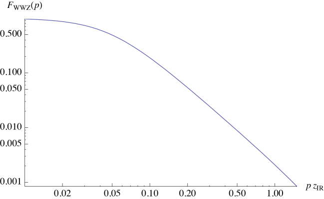
Figure 3: The form factor $F_{WWZ}(p)$ in the spacelike region for $z_{IR}^{-1}$ = 1.8 TeV.

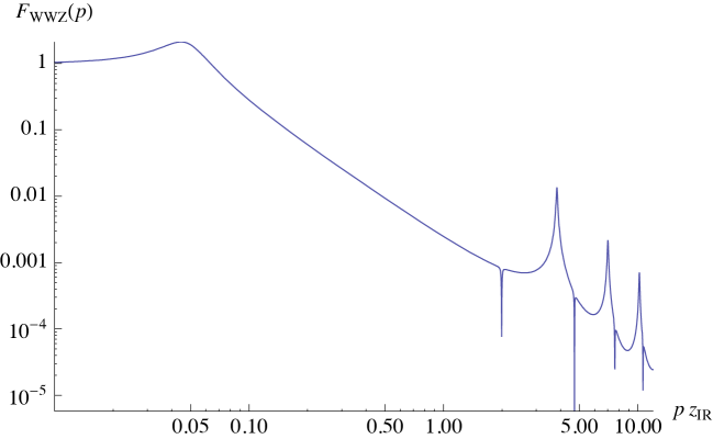
Figure 4: The form factor $F_{WWZ}(p)$ in the timelike region for $z_{IR}^{-1}$ = 1.8 TeV. The pole structure corresponds to the photon and $Z$-boson KK modes.

In Figure 3 the form factor in the spacelike region monotonously decreases as $p$ increases. This behavior also occurs in the timelike region in Figure 4, except that it is interspersed with periodic peaks and troughs. The position of every peak and trough coincides exactly with the KK mass poles: peaks are KK $Z$-bosons, while troughs are KK photons. This form factor structure can be compared with that expected from a confining gauge theory with a gravity dual, namely [41]

$$F_{ab}(q^{2})=\displaystyle\sum_{n=1}\frac{f_{n}g_{nab}}{q^{2}+m_{n}^{2}},$$ (B.14)

where $F_{ab}(q^{2})$ is the form factor associated with a spin-1 current for two external hadrons $a,b$, with coupling $g_{nab}$ to an $n$th vector hadron state with mass $m_{n}$ and decay constant $f_{n}$. This expression shows that in a confining gauge theory with large ‘t Hooft coupling, the form factor can be written as a sum over vector-meson poles. Our results are consistent with this formal prediction: a simple analytic fit in the low energy region ($Z$-pole dominant) for both the timelike and spacelike form factor gives $m_{Z}^{2}/(m_{Z}^{2}+p^{2})$, which appears as Eq.(60).

Note that although it is difficult to find a global fit for the structure of the time-like region, this fit is good in the low-energy region (smooth out the peak at $Z$ pole) which is monotonous and more relevant for LHC study. Interestingly a similar pole structure was originally conjectured for QCD by Sakurai [60, 41], where it was suggested that the form factor of an isospin-hadron $H$ is given by the $\rho$ meson pole: $F(q^{2})\approx\frac{f_{\rho}g_{\rho HH}}{q^{2}+m_{\rho}^{2}}$. For practical application, we can show that based on kinematics in high-energy scattering the momentum transferred in the $t$-channel is mostly spacelike, while in the $s$-channel it is always timelike.

References

- [1] D. B. Kaplan and H. Georgi, Phys. Lett. B 136, 183 (1984).
- [2] K. Agashe, R. Contino and A. Pomarol, Nucl. Phys. B 719, 165 (2005) [arXiv:hep-ph/0412089].
- [3] C. Csaki, C. Grojean, L. Pilo and J. Terning, Phys. Rev. Lett. 92, 101802 (2004) [arXiv:hep-ph/0308038].
-
[4]
L. F. Abbott and E. Farhi,
Phys. Lett. B 101, 69 (1981).
H. Fritzsch, D. Schildknecht and R. Kogerler, Phys. Lett. B 114, 157 (1982).
T. Kugo, S. Uehara and T. Yanagida, Phys. Lett. B 147, 321 (1984).
S. Uehara and T. Yanagida, Phys. Lett. B 165, 94 (1985).
M. Bando, T. Kugo and K. Yamawaki, Prog. Theor. Phys. 73, 1541 (1985).
M. Suzuki, Phys. Rev. D 37, 210 (1988).
M. Bando, T. Kugo and K. Yamawaki, Phys. Rept. 164, 217 (1988). - [5] M. Bando, T. Kugo, S. Uehara, K. Yamawaki and T. Yanagida, Phys. Rev. Lett. 54, 1215 (1985).
- [6] D. J. Gross, In *Liu, C.S. (ed.): Yau, S.T. (ed.): Chen Ning Yang* 147-162.
- [7] N. Seiberg, Int. J. Mod. Phys. A 16, 4365 (2001) [arXiv:hep-th/9506077].
- [8] J. M. Maldacena, Adv. Theor. Math. Phys. 2, 231 (1998) [Int. J. Theor. Phys. 38, 1113 (1999)] [arXiv:hep-th/9711200].
- [9] N. Arkani-Hamed, M. Porrati and L. Randall, JHEP 0108, 017 (2001) [arXiv:hep-th/0012148].
- [10] L. Randall and R. Sundrum, Phys. Rev. Lett. 83, 3370 (1999) [arXiv:hep-ph/9905221].
- [11] C. Amsler et al. [Particle Data Group], Phys. Lett. B 667, 1 (2008).
- [12] H. Georgi, A. K. Grant and G. Hailu, Phys. Lett. B 506, 207 (2001) [arXiv:hep-ph/0012379].
- [13] H. Davoudiasl, J. L. Hewett, B. Lillie and T. G. Rizzo, JHEP 0405, 015 (2004) [arXiv:hep-ph/0403300].
- [14] C. Csaki, J. Hubisz and P. Meade, arXiv:hep-ph/0510275.
- [15] G. R. Dvali, G. Gabadadze and M. A. Shifman, Phys. Lett. B 497, 271 (2001) [arXiv:hep-th/0010071].
- [16] M. S. Carena, T. M. P. Tait and C. E. M. Wagner, Acta Phys. Polon. B 33, 2355 (2002) [arXiv:hep-ph/0207056].
- [17] M. S. Carena, E. Ponton, T. M. P. Tait and C. E. M. Wagner, Phys. Rev. D 67, 096006 (2003) [arXiv:hep-ph/0212307].
- [18] Z. Chacko, M. A. Luty and E. Ponton, JHEP 0007, 036 (2000) [arXiv:hep-ph/9909248].
- [19] E. Ponton and E. Poppitz, JHEP 0106, 019 (2001) [arXiv:hep-ph/0105021].
- [20] H. Davoudiasl, J. L. Hewett and T. G. Rizzo, Phys. Rev. D 68, 045002 (2003) [arXiv:hep-ph/0212279].
- [21] R. Sundrum, Phys. Rev. D 59, 085009 (1999) [arXiv:hep-ph/9805471].
- [22] F. del Aguila, M. Perez-Victoria and J. Santiago, JHEP 0302, 051 (2003) [arXiv:hep-th/0302023].
- [23] S. B. Giddings, S. Kachru and J. Polchinski, Phys. Rev. D 66, 106006 (2002) [arXiv:hep-th/0105097].
- [24] Y. Grossman and M. Neubert, Phys. Lett. B 474, 361 (2000) [arXiv:hep-ph/9912408].
- [25] T. Gherghetta and A. Pomarol, Nucl. Phys. B 586, 141 (2000) [arXiv:hep-ph/0003129].
-
[26]
N. Arkani-Hamed, M. Porrati and L. Randall,
JHEP 0108, 017 (2001)
[arXiv:hep-th/0012148].
R. Rattazzi and A. Zaffaroni, JHEP 0104, 021 (2001) [arXiv:hep-th/0012248].
M. Perez-Victoria, JHEP 0105, 064 (2001) [arXiv:hep-th/0105048]. - [27] K. Agashe and A. Delgado, Phys. Rev. D 67, 046003 (2003) [arXiv:hep-th/0209212].
- [28] N. Seiberg, Nucl. Phys. B 435, 129 (1995) [arXiv:hep-th/9411149].
- [29] M. Harada and K. Yamawaki, Phys. Rept. 381, 1 (2003) [arXiv:hep-ph/0302103].
- [30] G. Cacciapaglia, C. Csaki, C. Grojean and J. Terning, Phys. Rev. D 70, 075014 (2004) [arXiv:hep-ph/0401160].
- [31] [LEP Collaborations], Phys. Rept. 427, 257 (2006) [arXiv:hep-ex/0509008].
- [32] M. E. Peskin and T. Takeuchi, Phys. Rev. D 46, 381 (1992).
- [33] P. Sikivie, L. Susskind, M. B. Voloshin and V. I. Zakharov, Nucl. Phys. B 173, 189 (1980).
- [34] C. Csaki, J. Erlich and J. Terning, Phys. Rev. D 66, 064021 (2002) [arXiv:hep-ph/0203034].
- [35] K. Agashe, A. Delgado, M. J. May and R. Sundrum, JHEP 0308, 050 (2003) [arXiv:hep-ph/0308036].
- [36] G. Cacciapaglia, C. Csaki, C. Grojean and J. Terning, Phys. Rev. D 71, 035015 (2005) [arXiv:hep-ph/0409126].
- [37] K. Agashe et al., Phys. Rev. D 76, 115015 (2007) [arXiv:0709.0007 [hep-ph]].
- [38] B. W. Lee, C. Quigg and H. B. Thacker, Phys. Rev. D 16, 1519 (1977).
- [39] J. F. Gunion, H. E. Haber, G. L. Kane and S. Dawson, The Higgs Hunter’s Guide, Westview Press (2000), 348pp.
- [40] S. J. Brodsky and G. F. de Teramond, Phys. Rev. D 77, 056007 (2008) [arXiv:0707.3859 [hep-ph]].
- [41] S. Hong, S. Yoon and M. J. Strassler, JHEP 0604, 003 (2006) [arXiv:hep-th/0409118].
- [42] K. Agashe and R. Contino, Nucl. Phys. B 742, 59 (2006) [arXiv:hep-ph/0510164].
- [43] M. Konyushikhin, arXiv:0906.1904 [hep-ph].
- [44] J. Polchinski and M. J. Strassler, Phys. Rev. Lett. 88, 031601 (2002) [arXiv:hep-th/0109174].
- [45] L. F. Alday and J. M. Maldacena, JHEP 0706, 064 (2007) [arXiv:0705.0303 [hep-th]].
- [46] J. McGreevy and A. Sever, JHEP 0802, 015 (2008) [arXiv:0710.0393 [hep-th]].
- [47] J. Polchinski and M. J. Strassler, JHEP 0305, 012 (2003) [arXiv:hep-th/0209211].
-
[48]
T. G. Rizzo,
Phys. Rev. D 32, 43 (1985).
M. Suzuki, Phys. Lett. B 153, 289 (1985).
J. A. Robinson and T. G. Rizzo, Phys. Rev. D 33, 2608 (1986).
G. Couture and J. N. Ng, Z. Phys. C 32, 579 (1986) [Erratum-ibid. C 43, 522 (1989)]. - [49] K. Hagiwara, R. D. Peccei, D. Zeppenfeld and K. Hikasa, Nucl. Phys. B 282, 253 (1987).
- [50] K. Hagiwara, J. Woodside and D. Zeppenfeld, Phys. Rev. D 41, 2113 (1990).
- [51] J. Alcaraz et al. [LEP Collaborations], arXiv:hep-ex/0612034.
- [52] I. Iashvili [CDF and D0 Collaborations], arXiv:0809.2955 [hep-ex].
- [53] ATLAS Collaboration, vol. II, CERN-LHCC-99-15, ATLAS-TDR-15 (May 1999).
-
[54]
R. N. Cahn, S. D. Ellis, R. Kleiss and W. J. Stirling,
Phys. Rev. D 35, 1626 (1987).
R. Kleiss and W. J. Stirling, Phys. Lett. B 200, 193 (1988).
V. D. Barger, T. Han and R. J. N. Phillips, Phys. Rev. D 37, 2005 (1988).
V. D. Barger, K. m. Cheung, T. Han and D. Zeppenfeld, Phys. Rev. D 44, 2701 (1991) [Erratum-ibid. D 48, 5444 (1993)]. - [55] G. Aad et al. [The ATLAS Collaboration], arXiv:0901.0512 [hep-ex].
- [56] V. Brigljevic et al., J. Phys. G 34, N269 (2007).
- [57] T. G. Rizzo, arXiv:hep-ph/0610104.
- [58] J. Kumar and J. D. Wells, Phys. Rev. D 74, 115017 (2006) [arXiv:hep-ph/0606183].
- [59] A. Pomarol, Phys. Lett. B 486, 153 (2000) [arXiv:hep-ph/9911294].
- [60] J. J. Sakurai, Annals Phys. 11, 1 (1960).