Simulations of Recoiling Massive Black Holes in the Via Lactea Halo

Abstract

The coalescence of a massive black hole (MBH) binary leads to the gravitational-wave recoil of the system and its ejection from the galaxy core. We have carried out $N$-body simulations of the motion of a $M_{\rm BH}=3.7\times 10^{6}\,\,{\rm M_{\odot}}$ MBH remnant in the “Via Lactea I” simulation, a Milky Way sized dark matter halo. The black hole receives a recoil velocity of $V_{\rm kick}$ = 80, 120, 200, 300, and 400 $\,{\rm km\,s^{-1}}$ at redshift 1.5, and its orbit is followed for over 1 Gyr within a “live” host halo, subject only to gravity and dynamical friction against the dark matter background. We show that, owing to asphericities in the dark matter potential, the orbit of the MBH is highly non-radial, resulting in a significantly increased decay timescale compared to a spherical halo. The simulations are used to construct a semi-analytic model of the motion of the MBH in a time-varying triaxial Navarro–Frenk–White dark matter halo plus a spherical stellar bulge, where the dynamical friction force is calculated directly from the velocity dispersion tensor. Such a model should offer a realistic picture of the dynamics of kicked MBHs in situations where gas drag, friction by disk stars, and the flattening of the central cusp by the returning black hole are all negligible effects. We find that MBHs ejected with initial recoil velocities $V_{\rm kick}\mathrel{\hbox to0.0pt{\lower 3.0pt\hbox{$\mathchar 536\relax$}\hss}\raise 2.0pt\hbox{$\mathchar 318\relax$}}500\,\,{\rm km\,s^{-1}}$ do not return to the host center within a Hubble time. In a Milky Way-sized galaxy, a recoiling hole carrying a gaseous disk of initial mass $\sim M_{\rm BH}$ may shine as a quasar for a substantial fraction of its “wandering” phase. The long decay timescales of kicked MBHs predicted by this study may thus be favorable to the detection of off-nuclear quasar activity.

1 Introduction

Intermediate-mass black holes may have formed at redshift $z\mathrel{\hbox to0.0pt{\lower 3.0pt\hbox{$\mathchar 536\relax$}\hss}\raise 2.0pt\hbox{$\mathchar 318\relax$}}15$ at the bottom of shallow dark-matter potential wells (Madau & Rees, 2001). These seed holes may have grown through gas accretion and binary coalescences to become the supermassive variety that is ubiquitously found today at the center of nearby galaxies (Kormendy et al., 1995; Richtsone et al., 1998; Tremaine et al., 2002). In the context of cold dark matter (CDM) cosmologies, where large halos are assembled via the hierarchical assembly and accretion of smaller progenitors, close MBH binaries inevitably form in large numbers during cosmic history (Begelman et al., 1980; Volonteri et al., 2003). The presence of a MBH binary with separation $<1\,$kpc has been revealed by Chandra observations of the nucleus of NGC 6240 (Komossa et al., 2003; Max et al., 2007).

The Very Long Baseline Array (VLBA) discovery in the radio galaxy 0402+379 of a MBH binary system with a projected separation of just 7 pc and a combined mass of $\sim 1.5\times 10^{8}\,\,{\rm M_{\odot}}$ was reported by Rodriguez et al. (2006). A MBH binary may shrink owing to stellar and/or gas dynamical processes (e.g., Mayer et al., 2007) and finally coalesce when gravitational wave radiation dominates orbital energy losses.

Recent developments in numerical relativity (Pretorius, 2005; Campanelli et al., 2006; Baker et al., 2006a) have allowed several groups to simulate the coalescence phases of black hole binaries (Baker et al., 2006a; Herrmann et al., 2007; González et al., 2007). Gravitational wave emission is typically anisotropic because of asymmetries associated with the masses and spins of the black holes, and causes the center of mass of the system to recoil in order to balance the linear momentum carried away by gravitational radiation (Bekenstein, 1973; Fitchett & Detweiler, 1984; Favata et al., 2004). The recoil velocity $\vec{V}_{\rm kick}$ depends on the binary mass ratio $q_{b}=M_{1}/M_{2}<1$ on the dimensionless spin vectors of the pair $\vec{a}_{1}$ and $\vec{a}_{2}$ ($0<a_{i}<1$), and on the orbital parameters. All current numerical data on kicks can be fitted by (Baker et al., 2008)

$$\vec{V}_{\rm kick} = v_{m}\,\vec{e}_{x}+v_{\perp}(\cos\xi\,\vec{e}_{x}+\sin\xi\,\vec{e}_{y})+v_{\parallel}\,\vec{e}_{z},$$ (1)

$$v_{m} = A\mu^{2}\sqrt{1-4\mu}\,(1+B\mu),$$ (2)

$$v_{\perp} = H\mu^{2}(1+q_{b})^{-1}\left(a_{2}^{\parallel}-q_{b}a_{1}^{\parallel}\right),$$ (3)

$$v_{\parallel} = K\mu^{3}(1+q_{b})^{-1}[q_{b}a_{1}^{\perp}\cos(\phi_{1}-\Phi_{1})-a_{2}^{\perp}\cos(\phi_{2}-\Phi_{2})],$$ (4)

where $\mu=q_{b}/(1+q_{b})^{2}$ is the symmetric mass ratio, $\theta_{i}$ is the angle between the dimensionless spin vector $\vec{a}_{i}=\vec{S}_{i}/M_{i}^{2}$ of the $i$th black hole and orbital angular momentum vector, $\phi_{i}$ is a projection angle between the spin vectors and a reference angle that lies in the orbital plane, and $\Phi_{1}(q_{b})=\Phi_{2}(1/q_{b})$ are constant for a given value of $q_{b}$. Here, $A=1.35\times 10^{4}\,{\rm km\,s^{-1}}$, $B=-1.48$, $H=7540\pm 160\,{\rm km\,s^{-1}}$, $\xi=215^{\circ}\pm 5^{\circ}$, and $K=2.4\pm 0.4\times 10^{5}\,{\rm km\,s^{-1}}$. Assuming random spin orientations, $q_{b}>1/4$, and $a_{1}=a_{2}=0.9$, recoiling black holes can get a kick velocity $>500\,\,{\rm km\,s^{-1}}$ approximately 60% of the time (see Table 3 of Baker et al., 2008). For $q_{b}>0.1$, the percentage of kicks with $>500\,\,{\rm km\,s^{-1}}$ decreases to $\sim 20\%$. Spins that are aligned with the orbital angular momentum vector (as expected under the action of external torques provided by a circumbinary accretion flow, see Bogdanović et al. 2007) yield recoil velocities below $200\,\,{\rm km\,s^{-1}}$, while the configuration producing the maximum recoil kick corresponds to equal-mass maximally rotating holes with anti-aligned spins oriented parallel to the orbital plane, $V_{\rm kick}=K\mu^{3}=3750\,\,{\rm km\,s^{-1}}$ (Campanelli et al., 2007a).

If not ejected from the host altogether, the recoiling MBH will travel some maximum distance and then return to the center subject to dynamical friction (Madau & Quataert, 2004). Galaxy mergers are also a leading mechanism for supplying gas to their nuclear MBHs, and a recoiling hole can retain the inner parts of its accretion disk, providing fuel for a continuing luminous phase along its trajectory. Two possible observational manifestations of gravitational-radiation ejection have then been suggested: (1) spatially offset active galactic nuclei (AGN) activity (Madau & Quataert, 2004; Blecha & Loeb, 2008; Volonteri & Madau, 2008); and (2) broad emission lines that are substantially shifted in velocity relative to the narrow-line gas left behind (Bonning, Shields, & Salviander, 2007). The effect of gravitational wave recoil in the mass buildup of MBHs is more prominent at high redshifts (e.g., Volonteri & Rees, 2006; Tanaka & Haiman, 2009) and therefore the detection of offset nuclei is difficult. Observational evidence of recoiling MBHs is scarce and highly controversial. A recoiling SMBH candidate at z = 0.71 was reported by Komossa et al. (2008) in quasar SDSS J092712.65+294344.0. The broad-line region of the quasi-stellar object (QSO), powered by a $6\times 10^{8}M_{\odot}$ black hole, appeared to have a velocity offset of $2650\,\,{\rm km\,s^{-1}}$ with respect to the narrow-line region associated with the galaxy. However, several authors have challenged this hypothesis, proposing that the object is a MBH binary (Dotti et al., 2008; Bogdanović et al., 2009) or an interacting galaxy pair (Shields et al., 2009; Heckman et al., 2009).

The observability of recoiling MBHs depends sensitively on their dynamics in galaxy halos. The radial orbit of a recoiling hole in a spherically symmetric potential was first studied analytically by Madau & Quataert (2004) and numerically by Boylan-Kolchin et al. (2004). These early studies showed that large kicks ($\sim 400\,\,{\rm km\,s^{-1}}$) can displace MBHs tens of kiloparsecs away from the center of a Milky Way-sized stellar bulge and that, after the kick, the MBH undergoes several oscillations before decaying back to the bottom of the potential. Most of the orbital energy is lost during the MBH passages through the center, where dynamical friction is most efficient: the cuspy central stellar density profile is flattened by the heating effect of dynamical friction, and the MBH decay timescale correspondingly lengthened. Gualandris & Merritt (2008) have recently substantiated these results by performing direct summation $N$-body simulations of MBH recoil in spherical galaxies with binary-depleted cores. They found that initially the MBH loses its energy due to dynamical friction as predicted by Chandrasekhar’s theory (Chandrasekhar, 1943). When the amplitude of the motion has fallen to roughly the core radius, the MBH and core experience damped oscillations about their common center of mass, which decay until the hole reaches thermal equilibrium with the surrounding stars. Vicari et al. (2007) evaluated the effect of non-spherical galaxy geometries on kicked MBHs using triaxial models, and found significantly longer decay timescales than in equivalent spherical systems, as in a non-spherical potential the hole does not return directly through the dense center where the dynamical friction force is highest. Blecha & Loeb (2008) studied the trajectories of kicked holes in a two-component galaxy model that includes a spherical stellar bulge and a gaseous disk, and found that kicks with initial velocity $V_{\rm kick}\mathrel{\hbox to0.0pt{\lower 3.0pt\hbox{$\mathchar 536\relax$}\hss}\raise 2.0pt\hbox{$\mathchar 316\relax$}}200\,\,{\rm km\,s^{-1}}$ in the plane of the disk are quickly damped out in $t\mathrel{\hbox to0.0pt{\lower 3.0pt\hbox{$\mathchar 536\relax$}\hss}\raise 2.0pt\hbox{$\mathchar 316\relax$}}10^{6.5}$ yr.

In this paper, we revisit the problem using a different approach. We carry out full $N$-body simulations of a recoiling MBH that is subject only to gravity and dynamical friction against the dark matter background, in a high-resolution, non-axisymmetric, “live” potential. The host is the main halo of the Via Lactea I (hereafter VL-I) cosmological simulation (Diemand et al. 2007a, 2007b). We follow the MBH orbital behavior starting at redshift $z=1.5$ (when the kick is assumed to occur) for more than 1 Gyr, as the host grows in mass and changes its shape from prolate to triaxial. We show that, owing to departures from axisymmetry in the dark matter potential, the orbit of the hole is highly non-radial, resulting in a significantly increased decay timescale compared to a spherical halo. The simulations are used to construct a more realistic semi-analytic model of the motion of the MBH in a time-varying triaxial Navarro–Frenk–White (NFW) halo plus a fixed isothermal stellar bulge, where the dynamical friction force is calculated directly from the velocity dispersion tensor. Such a model should offer a more realistic picture of the dynamics of kicked MBHs in situations where gas drag, friction by disk stars, and the heating effect of the returning hole on the central cusp are all negligible.

2 Simulations setup and properties of the host

The VL-I simulation was performed with PKDGRAV (Stadel 2001) a cosmological tree code that includes gravitational multipoles up to hexa-decapole order to reach high accuracy in the force calculation. It employed multiple mass particle grid initial conditions generated with the GRAFIC2 package (Bertschinger, 2001) in a WMAP 3-year cosmology (Spergel et. al, 2007). A bug in the original GRAFIC2 code caused the power spectrum used for the VL-I refinements to be that of the baryonic component, equivalent to an effective spectral index of $n=0.90$ instead of the intended 0.95. In this cosmology subhalo concentrations and peak circular velocities are slightly lower than in WMAP 3-year, while $\sigma_{8}$ and the main halo properties remain the same.  The high-resolution region was sampled with 234 million particles of mass $m_{p}=2.1\times 10^{4}\,{\rm M_{\odot}}$ and evolved with a force resolution of $\epsilon=90$ pc. It was embedded within a periodic box of comoving size $L=90$ Mpc, which was sampled at lower resolution to account for the large-scale tidal forces. The host halo mass at $z=0$ is $M_{200}=1.8\times 10^{12}\,\,{\rm M_{\odot}}$ within a radius of $R_{200}=389$ kpc (defined as the radius within which the enclosed average density is 200 times the mean matter value). In this work we rerun VL-I using PKDGRAV from redshift $z_{i}=1.54$ to $z_{f}=1.15$, and follow the orbits of all dark matter particles as well as a new MBH particle placed at the center of the host. As in the original VL-I simulation, we employ a gravitational softening of 90 pc for the dark matter particles and the MBH, as well as adaptive time steps as short as $\tau=68,500$ yr, sufficient to ensure convergence in the density profile down to a radius of $r_{\rm conv}\sim 1.0$ kpc and to accurately sample the orbit of the MBH. The time-stepping criterion is given by $\Delta t<0.2\sqrt{\epsilon/a_{l}}$, where $a_{l}$ is the local acceleration. The resolution of VL-I allows us to adopt the mass of SgrA*, $M_{\rm BH}=3.7\times 10^{6}\,\,{\rm M_{\odot}}$ (Ghez et al., 2005), for the central MBH particle: this implies a MBH-to-particle mass ratio of 175, enough to accurately reproduce the effect of dynamical friction.

Large kicks can displace MBHs sufficiently far away that their decay times become a significant fraction of the age of the universe. It is interesting to look at the evolution of the host halo in terms of its time-varying spherically averaged density profile and shape parameters. The fitting formula proposed by Navarro et al. (1997) provides a reasonable approximation to the density profile,

$$\rho(x)=\frac{\rho_{s}}{x(1+x)^{2}},$$ (5)

where $x=r/R_{s}$ and $R_{s}$ is the scale radius. The mass profile is given by $M(<x)=M_{200}f(x)/f(c)$, where $f(x)\equiv\ln(1+x)-x/(1+x)$ and $c\equiv R_{200}/R_{s}$ is the concentration parameter. The escape speed from the halo center is

$$v_{\rm esc}^{2}(0)=2\int_{0}^{\infty}\frac{GM(<r)}{r^{2}}\,dr=\frac{2V_{200}^{2}c}{f(c)},$$ (6)

where $V_{200}^{2}\equiv GM_{200}/R_{200}$. The quantities $\rho_{s},R_{s},R_{200},M_{200}$, $V_{\rm max}$ (the maximum circular velocity of the host) and $v_{\rm esc}(0)$ are given in Table 1 at different scale factors, starting with the time when the kick is imparted.

CDM halos are known to show significant departures from sphericity (for a recent summary, see Allgood et al. 2006). As detailed in Kuhlen et al. (2007), we approximate the shape of the VL-I host potential by diagonalizing the unweighted kinetic energy tensor

$$K_{ij}=\frac{1}{2}\sum_{n}v_{i,n}v_{j,n},$$ (7)

where $K_{ij}$ is related to the potential energy tensor $W_{ij}=\sum x_{i}d\Phi/dx_{j}$ through the tensor virial theorem

$$\frac{1}{2}\frac{d^{2}I_{ij}}{dt^{2}}=2K_{ij}+W_{ij}.$$ (8)

Here,

$$I_{ij}=\sum_{n}\frac{x_{i,n}x_{j,n}}{r^{2}_{n}}.$$ (9)

and $r_{n}=\sqrt{(x_{n}^{2}+(y_{n}/q)^{2}+(z_{n}/s)^{2})}$. We assume $d^{2}I_{ij}/dt^{2}=0$ so that the eigenvectors of $K_{ij}$ reflect the principal axes of the potential ellipsoid. The latter is significantly rounder than the mass distribution, and neither its shape nor orientation varies much with the radius (Kuhlen et al., 2007). The degree of triaxiality of the halo potential, $T$, is given by (Franx et al., 1991)

$$T=\frac{1-q^{2}}{1-s^{2}},$$ (10)

where $q=b/a$ and $s=c/a$ are the time-dependent intermediate-to-major and minor-to-major axis ratios, respectively ($a\geq b\geq c$). A halo is said to be oblate for $T<1/3$, triaxial for $1/3<T<2/3$, and prolate for $T>2/3$. Figure 1 shows the evolution of the potential shape parameters with redshift at different radii. In the inner regions the axis ratios remain approximately constant after around $z=0.8$, but before $z=1$ there are significant changes in the outer regions, as the halo becomes more spherical. The triaxiality parameter remains mostly in the prolate regime ($>2/3$) in the inner regions, while in the outer halo evolves from prolate at $z\mathrel{\hbox to0.0pt{\lower 3.0pt\hbox{$\mathchar 536\relax$}\hss}\raise 2.0pt\hbox{$\mathchar 318\relax$}}1$ to triaxial or slightly oblate at $0.7\mathrel{\hbox to0.0pt{\lower 3.0pt\hbox{$\mathchar 536\relax$}\hss}\raise 2.0pt\hbox{$\mathchar 316\relax$}}z\mathrel{\hbox to0.0pt{\lower 3.0pt\hbox{$\mathchar 536\relax$}\hss}\raise 2.0pt\hbox{$\mathchar 316\relax$}}1$, to back to prolate at later times. Note that the VL-I host accretes some fairly massive subhalos between $z=1$ and $z=0.5$. Dynamical friction causes these subhalos to spiral in to the center over a few orbits, and they lose most of their mass in this process. The associated redistribution of material probably contributes to the observed shape adjustments.

3 Dynamics of recoiling holes

3.1 Orbits in numerical simulations

We placed the MBH particle at the position of the densest point of the main VL-I halo at an initial redshift $z_{i}=1.54$, 300 Myr after the last major merger. At this epoch the host has $M_{200}=1.02\times 10^{12}\,\,{\rm M_{\odot}}$ and $R_{200}=187$ kpc. The kick was oriented at an angle of 20^∘ to the minor axis of the host halo at $z_{i}$. The MBH orbit was tracked at every time step in our simulations, and its position and velocity were measured with respect to the central position and center of mass velocity, respectively. The five halo$+$MBH runs —corresponding to kick velocities $V_{\mathrm{kick}}$ = 80, 120, 200, 300, and 400 $\,{\rm km\,s^{-1}}$ and labeled VL080 to VL400— were evolved for 1.15 Gyr (i.e., until a final redshift $z_{f}=1.15$). All kick velocities are below the escape speed at $z_{i}$, $v_{\rm esc}(r=0,z_{i})=488\,\,{\rm km\,s^{-1}}$. Each run consumed 13,000 CPU hours on the Pleiades Supercomputer Cluster at UCSC, and followed the MBH for 10,000 time steps.

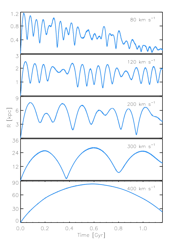
Figure 2: Response of a $M_{\rm BH}=3.7\times 10^{6}\,\,{\rm M_{\odot}}$ MBH to a kick at $z_{i}=1.54$ in the aspherical potential of the “live” VL-I Milky Way-sized halo. The radial distance $R$ of the hole from the center is plotted vs. time for $V_{\mathrm{kick}}$ = 80, 120, 200, 300, and 400 $\,{\rm km\,s^{-1}}$. Each orbit was sampled with 10,000 points.

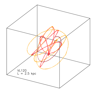
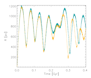
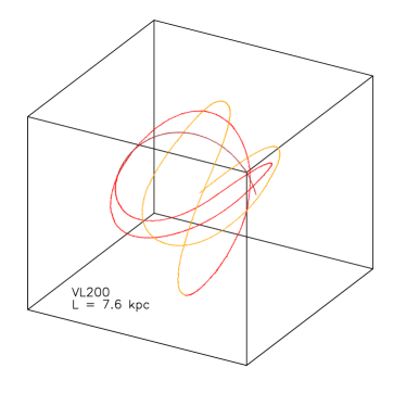
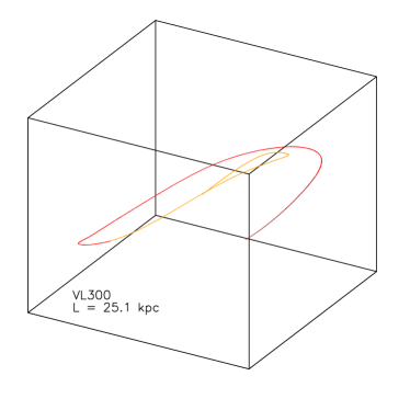
Figure 3: Left top, left bottom, and right bottom panels: Three-dimensional orbits of the recoiling MBHs in the VL120, VL200, and VL300 simulations. The first 0.5 Gyr are plotted in yellow, the following 0.5 Gyr in red, and the remaining 0.1 Gyr in purple. Box sizes are 2.5, 7.6, and 25.1 kpc, respectively. Right top panel: Comparison between orbits in VL080 (yellow) and the corresponding energy-conserving orbits in the massless hole simulation (green).

The resulting trajectories are shown in Figure 2, the orbits’ parameters are listed in Table 2, and the three-dimensional rendering of the orbits in simulations VL120, VL200, and VL300 are shown in Figure 3. Only $V_{\rm kick}>300\,\,{\rm km\,s^{-1}}$ trajectories actually sample the outer halo with pericenter distances $R_{\rm max}\mathrel{\hbox to0.0pt{\lower 3.0pt\hbox{$\mathchar 536\relax$}\hss}\raise 2.0pt\hbox{$\mathchar 318\relax$}}30$ kpc, and only $V_{\rm kick}<120\,\,{\rm km\,s^{-1}}$ trajectories return within 0.5 kpc from the center during the duration of the simulation. The motion of the hole remains nearly rectilinear for one or two oscillations only, as the $y$- and $z$-components of its orbit become rapidly important due to asphericities in the halo potential. This increases the MBH decay timescale compared to a spherical model, as we show below. Dynamical friction has only a weak effect on the maximum displacement of the MBH. This can be seen in Figure 3 (right top panel), where a sixth simulation was carried out with the recoiling hole treated as a massless test particle of initial kick velocity $V_{\mathrm{kick}}=80\,\,{\rm km\,s^{-1}}$. A comparison with VL080 shows how, for the first 2-3 oscillations, dynamical friction does not strongly influence the motion of the hole, and the maximum displacement is similar to that of the energy-conserving orbit. It is only at later times that the effect of friction sets in, reducing the amplitude and period of the oscillations and bringing the hole back to the center. Note how, for $V_{\rm kick}\geq 120\,\,{\rm km\,s^{-1}}$, and because of the aspheric nature of the halo, the MBH spends most of its time $>0.8$ kpc away from the center and does not have a significant dynamical heating effect on the dark matter distribution in the nucleus.

3.2 Orbits in a spherical NFW halo

It is interesting at this stage to compare the results of our numerical simulations with a semi-analytic model of the motion of a recoiling MBH in an NFW halo. Such a model will allow us to follow the trajectory of a recoiling black hole for a Hubble time or until it returns to the center. We define the return time, $t_{\rm return}$, as the time it takes for the MBH to decay to within $r=1$ pc of the center of the halo with $|E/E_{\rm in}|<0.001$, where $E$ is the total energy (kinetic + potential) of the MBH and $E_{\rm in}$ is its initial energy. The energy condition is set to ensure that the MBH is not simply going through a close periastron passage.

We start by approximating the potential as spherically symmetric and static, with the $z=0$ host halo parameters given in Table 1. Under these assumptions the trajectory is purely radial, and the damping force from the background dark matter can be approximated by the classical Chandrasekhar dynamical friction formula (Chandrasekhar, 1943; Binney & Tremaine, 1987). The corresponding equation of motion is

$$\frac{d\vec{v}}{dt}=-\frac{GM(<r)}{r^{3}}{\vec{r}}-\frac{4\pi G^{2}\ln\Lambda\rho(r)M_{\mathrm{BH}}}{v^{3}}\left[{\rm erf}(X)-\frac{2X}{\sqrt{\pi}}e^{-X^{2}}\right]\vec{v},$$ (11)

where $X\equiv v/\sqrt{2}\sigma$.

The proper definition of the Coulomb logarithm, $\ln\Lambda$, has been extensively debated. It is generally defined as $\ln\left(b_{\mathrm{max}}/b_{\mathrm{min}}\right)$, where the maximum impact parameter $b_{\mathrm{max}}$ is the scale radius $R_{s}$ of the dark matter distribution, and the minimum impact parameter $b_{\mathrm{min}}$ is the radius of influence of the MBH, $R_{\rm BH}=GM_{\rm BH}/\sigma^{2}$. Several studies (e.g., Colpi et al., 1999; Hashimoto et al., 2003) have shown that a dynamically varying value for $\ln\Lambda$ provides a better estimate of dynamical friction than a constant value when compared to $N$-body simulations. Here we follow the treatment of Maoz (1993), and in the approximation of a spherical NFW host write the Coulomb logarithm as

$$\ln\Lambda\rightarrow\int_{d}^{R_{s}}\frac{\rho(r)}{\rho_{0}r}\,dr=\frac{\rho_{s}}{\rho_{0}}\int_{x_{0}}^{1}\frac{\,dx}{x^{2}(1+x)^{2}}=\frac{\rho_{s}}{\rho_{0}}\left[2\ln\left(\frac{x+1}{x}\right)-\frac{2x+1}{x(x+1)}\right]^{1}_{x_{0}},$$ (12)

where $\rho_{0}$ is the central mass density, $x=r/R_{s}$, $d$ can be interpreted as the minimum impact parameter of the Chandrasekhar formula. Throughout this paper we use $\rho_{0}=\rho(r={\rm 20\,pc})$ and set $d=R_{\rm BH}$, the radius of influence of the MBH.

The one-dimensional velocity dispersion $\sigma$ for an NFW profile can be solved numerically from the Jeans equation or approximated analytically for $x=r/R_{s}$ between 0.01 and 100 by the function (Zentner & Bullock, 2003)

$$\sigma^{2}(x) = V_{200}^{2}\frac{c}{f(c)}x(1+x^{2})\int_{x}^{\infty}\frac{f(x^{\prime})}{x^{\prime 3}(1+x^{\prime})^{2}}\,dx^{\prime}$$ (13)

$$\simeq V_{\mathrm{max}}^{2}\left(\frac{1.4393x^{0.354}}{1+1.1756x^{0.725}}\right)^{2}.$$ (14)

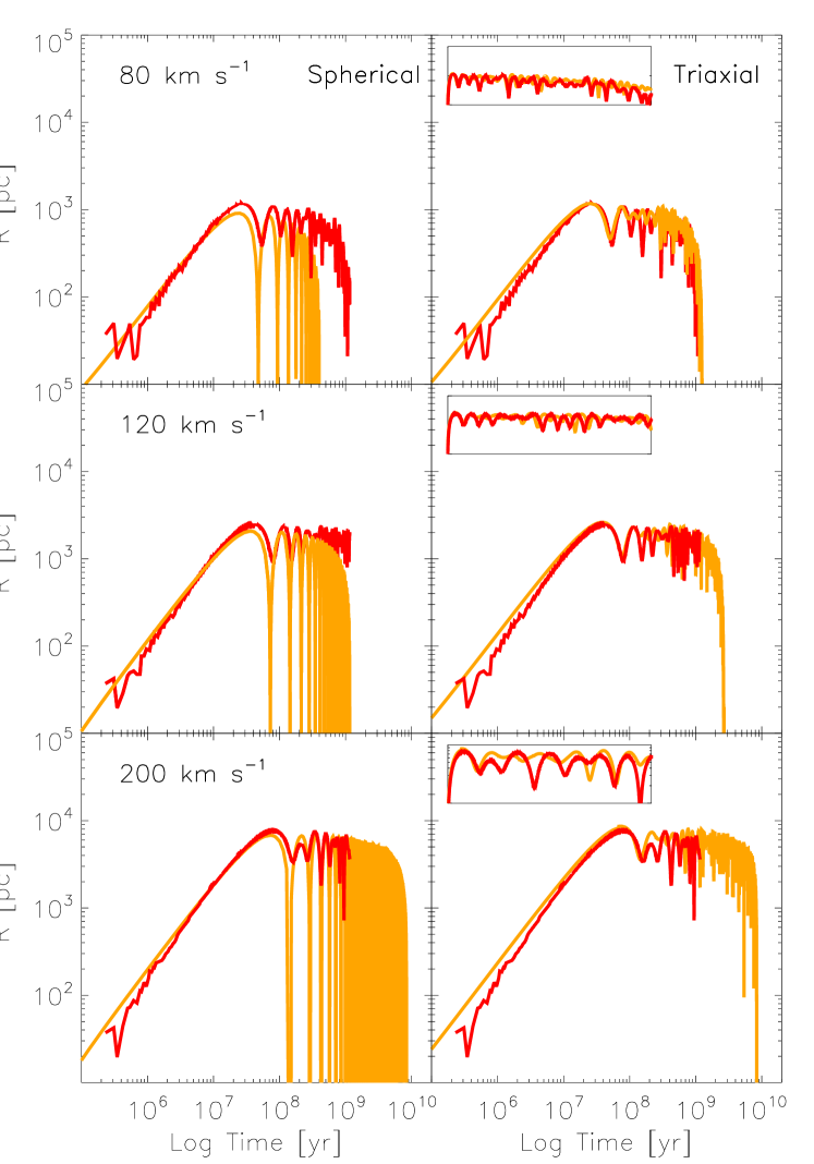
Figure 4: Decay histories of recoling MBHs. The radial distance $R$ from the center is plotted as a function of time for a spherical NFW (left panel) and a triaxial NFW halo (right panel). The $N$-body simulation results (red curves) are superposed to the semi-analytic orbit integrations according to model A (orange). The insets are a close-up of the respective orbit over a timescale of 1.1 Gyr.

We integrate the equation of motion numerically using an adaptive Adams-Bashforth-Moulton integration scheme. The resulting radial orbits for kick velocities $V_{\mathrm{kick}}=80,120$, and $200\,\,{\rm km\,s^{-1}}$ are shown in Figure 4 (left panels). The decay timescale of a recoiling hole in a spherical potential is significantly shorter compared to the results of $N$-body simulations, mainly because of the efficiency of dynamical friction during each passage through the nuclear regions. In the $V_{\rm kick}=120\,\,{\rm km\,s^{-1}}$ case, for example, the MBH is back to the center after 0.6 Gyr in the spherical case, while it is still wandering close to $R_{\rm max}$ in the simulations. A self-consistent estimate of the decay timescale must include the flattening of the cuspy central density profile by the oscillating hole. Such a cumulative heating effect, however, is negligible in this case, since due to the triaxiality of the potential the MBH does not affect the central density and velocity dispersion profiles dramatically.

3.3 Orbits in a triaxial NFW halo

The next-order approximation is to model the motion of the recoiling hole in a triaxial, dynamically evolving NFW dark matter halo, using the VL-I halo parameters given in Table 1 and the potential shape parameters plotted in Figure 1. The orbit of the hole is fully specified by the conservative force of the dark matter potential $\nabla\Phi$ and the damping frictional term:

$$\frac{d\vec{v}}{dt}=-\vec{\nabla}\Phi+\vec{f}_{\mathrm{DF}},$$ (15)

where

$$\Phi=-\frac{GM_{200}}{f(c)}\frac{\ln(1+r_{e}/R_{s})}{r_{e}},$$ (16)

and

$$r_{e}\equiv\left(x^{2}+\frac{y^{2}}{q^{2}}+\frac{z^{2}}{s^{2}}\right)^{1/2}$$ (17)

is the ellipsoidal radius. Here $q$ and $s$ are the time- and radial-dependent axis ratios defined in Section 2, and $x,y,z$ are Cartesian coordinates along the principal axis of the potential ellipsoid. Equation (11) is no longer valid in a triaxial system, where the velocity dispersion is non-isotropic and the velocity distribution deviates from Maxwellian. We adopt the Pesce et al. (1992) generalization of the dynamical friction formula to triaxial systems (see also Vicari et al., 2007),

$$\vec{f}_{\rm DF}=-\Gamma_{a}V_{a}\hat{e}_{a}-\Gamma_{b}V_{b}\hat{e}_{b}-\Gamma_{c}V_{c}\hat{e}_{c},$$ (18)

where $V_{i}$ are the components of the black hole velocity along the principal axes $\hat{e}_{i}=\{\hat{e}_{a},\hat{e}_{b},\hat{e}_{c}\}$ of the local velocity dispersion ellipsoid with $a>b>c$, and $\Gamma_{i}$ are the dynamical friction coefficients. These are given by

$$\Gamma_{i}=\frac{2\sqrt{2\pi}G^{2}\rho(r_{e})\ln\Lambda(M_{\mathrm{BH}})}{\sigma_{1}^{3}}\times B_{i}(\vec{V},{\bf\sigma}),$$ (19)

where the velocity dispersion integral is given by

$$B_{i}=\int_{0}^{\infty}\frac{\exp(-\sum_{i=1}^{3}\frac{V_{i}^{2}/2\sigma_{i}^{2}}{\epsilon_{i}^{2}+u})}{\sqrt{(\epsilon_{1}^{2}+u)(\epsilon_{2}^{2}+u)(\epsilon_{3}^{2}+u)}}\frac{1}{\epsilon_{i}^{2}+u}\,du,$$ (20)

$\epsilon_{i}\equiv\sigma_{i}/\sigma_{1}$, $\sigma_{i}^{2}=\{\sigma_{a}^{2},\sigma_{b}^{2},\sigma_{c}^{2}\}$ is the velocity dispersion along the direction $\{\hat{e}_{a},\hat{e}_{b},\hat{e}_{c}\}$, $\sigma_{1}$ is the largest eigenvalue, and $\rho(r_{e})$ is the local mass density at the MBH’s elliptical radius. In order to calculate the triaxial density profile, we deform the spherical density contours in such a way that the volume is preserved. In this approximation, the characteristic elliptical radius of the halo becomes $R_{e,200}=(q\,s)^{-1/3}R_{200}$.

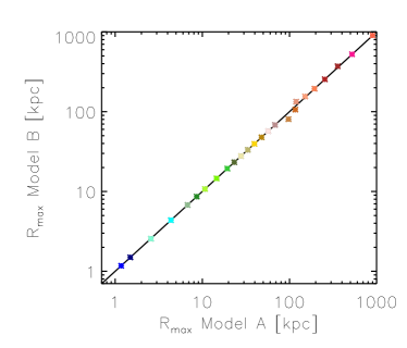
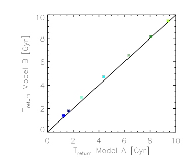
Figure 6: Left: Maximum displacement distance in model A (fiducial) compared to model B for kick velocities in the range $80<V_{\mathrm{kick}}<600\,\,{\rm km\,s^{-1}}$ (asterisks). Right: Return times of models A and B for kick velocities $80<V_{\mathrm{kick}}<250\,\,{\rm km\,s^{-1}}$ (asterisks). Colors represent magnitude of the recoil velocity from $V_{\rm kick}=80\,\,{\rm km\,s^{-1}}$ (blue) to $V_{\rm kick}=600\,\,{\rm km\,s^{-1}}$ (red).

A correct estimate of the velocity dispersion as a function of radius and redshift is crucial in the calculation of dynamical friction. Here, we take the following approach. First, we measure the “true” shape and orientation of the local velocity dispersion ellipsoids directly from the VL-I simulation (model A; see Section  3.3.1 for details). Next, we construct a model to calculate the velocity dispersion from the Jeans equation (model B; see Section 3.3.2). In model B we neglect streaming motions and assume that the local velocity dispersion ellipsoids are aligned with the global potential shape, which results in an overestimate of the velocity dispersion integral $B_{i}$ given by Equation 20. To normalize model B to the fiducial model A, we introduce a linear fitting factor $\eta$ where $B_{i}^{\rm model\,A}=\eta B_{i}^{\rm model\,B}$. The main characteristics of the MBH orbits are well reproduced by models A and B for a large range of recoil velocities using $\eta=0.5$ (see Figure 6).

The resulting orbits are shown in the right panels of Figure 4. The triaxial halo model qualitatively reproduces the results of the simulations, the highly non-radial MBH trajectories, and the extended wandering times of kicked holes. Return timescales exceed 10 Gyr already for $V_{\rm kick}=200\,\,{\rm km\,s^{-1}}$ (see the last column of Table 2).

3.3.1 Model A: Local Velocity Dispersions Measured in VL-I

The local properties of the halo relevant to the calculation of dynamical friction were measured from the VL-I simulation as a function of redshift for 10 snapshots in the range $0<z<1.54$, following the method of Zemp et al. (2009). At each redshift seven distances $r=1,8,25,50,100,200,400$ kpc from the halo center were randomly sampled with 10 spheres of radius

$$r_{\mathrm{sph}}(r)=r_{\mathrm{sph}}(8\,\mathrm{kpc})\left[\frac{\rho(8\,\mathrm{kpc})}{\rho(r)}\right]^{1/3},$$ (21)

where $r_{\mathrm{sph}}(8\,\mathrm{kpc})=0.5$ kpc and $\rho(r)$ is the spherically averaged mass density at radius $r$. In each sphere we measure the local density and calculate the six components of the symmetric velocity dispersion tensor, $\sigma_{ij}^{2}\equiv\langle v_{i}v_{j}\rangle-\langle v_{i}\rangle\langle v_{j}\rangle$ (here the indices $i$ and $j$ indicate the components along the principal axes of the global potential ellipsoid). We then diagonalize the dispersion tensor to obtain a set of eigenvalues and eigenvectors. The eigenvalues, $\{\sigma_{a}^{2},\sigma_{b}^{2},\sigma_{c}^{2}\}$, are the components of the velocity dispersion in the $\hat{e}_{i}$ basis.

For computational convenience, we fit an analytical function to the mean value of the local velocity dispersion in all spheres at each radii. This function has the form (Pesce et al., 1992) for model A:

$$\sigma_{i,A}^{2}(r)=A_{i}\left[\frac{1+B_{i}r^{m_{i}}}{1+D_{i}r^{n_{i}}}\right]e^{-r/{C_{i}}},$$ (22)

where $A_{i}$ through $D_{i}$ and $m_{i},n_{i}$ are the best fit values to the velocity dispersion profile in the $i$th direction at a given redshift. The parameters at $z=0$ are given in Table 3, and the corresponding best-fit curves for $\sigma_{i,A}$ are shown in Figure 5b.

The orientation of the local velocity ellipsoids with respect to the global shape was also measured as a function of radius and redshift. Table 4 shows the angles between the major, medium, and minor axes of the velocity dispersion ellipsoid and their counterparts in the global potential ellipsoid ($\bar{\alpha},\bar{\beta},\bar{\gamma}$ respectively) averaged over the ensemble of spheres. The principal axes of the velocity ellipsoid show significant misalignment with the principal axes of the global potential shape: the distribution of orientation angles is quite isotropic and cannot be fit by a simple function. In our fiducial semi-analytical model (model A), the orientation of the local velocity dispersion is obtained by interpolating a grid of mean orientation angles as a function of position and redshift at each time step of the numerical integration. Then a random value is drawn in the range allowed by the dispersion associated with the mean.

The local density profile is shown in Figure 5a. The points represent the average local measurement, $\bar{\rho}$, and the error bars are the dispersion around $\bar{\rho}$, labeled $\sigma(\bar{\rho})$ in Table 4. The solid line represents the best fit NFW profile to the local density average at $z=0$ (see Table 1).

3.3.2 Model B: A simple treatment of local velocity dispersion

While our fiducial model accurately reproduces important features of the orbits of MBHs in a triaxial potential, having a simple prescription to calculate the velocity dispersion analytically would allow us to generalize our model and include the effect of other galactic components (see below). In this toy model, we assume that the local velocity dispersion ellipsoids are aligned with the potential shape: therefore $\{\hat{e}_{a},\hat{e}_{b},\hat{e}_{c}\}=\{\hat{e}_{x},\hat{e}_{y},\hat{e}_{z}\}$ and all off-diagonal terms of the local velocity tensor vanish. We further assume that the halo is in steady state at each snapshot and that there are no streaming motions. Under these assumptions we solve for the velocity dispersion along the $i$th coordinate from a simplified Jeans equation:

$$\sigma^{2}_{i,B}=\frac{1}{\rho_{e}}\int_{x_{i}}^{\infty}\rho(r_{e})\frac{\partial\Phi(r_{e})}{\partial x^{\prime}_{i}}\,dx^{\prime}_{i},$$ (23)

where $\rho_{e}$ is the density at the elliptical radius corresponding to the position of the MBH. We normalize the velocity dispersion integral (Equation 20) to $\eta B_{i}(\vec{V},\vec{\sigma_{B}})$ in order to match the results of model A. Figure 6 shows a comparison of models A and B: maximum displacement distance and return times are accurately reproduced by model B for a large range of kick velocities with $\eta=0.5$. This analytical representation of the velocity dispersion in a triaxial potential proves useful in the construction of the composite potential described below.

3.4 Orbits in a triaxial NFW halo plus a stellar bulge

A realistic study of the trajectories of recoiling holes must include the gravitational and frictional effect of a stellar bulge. Our final set of semi-analytic orbit integrations uses a two-component galaxy model consisting of a time-varying triaxial halo (with same parameters as above) and a fixed spherical bulge of stellar density

$$\rho_{*}(r)=\frac{\sigma^{2}_{*}}{2\pi G(r^{2}+r_{c}^{2})},$$ (24)

with isotropic stellar velocity dispersion $\sigma_{*}=75\,\,{\rm km\,s^{-1}}$, suitable for a Milky-Way-sized host. In the inner regions of the bulge, where stars are the dominant source of dynamical friction, the sphere of influence of the black hole is given by $R_{\rm BH}=GM_{\rm BH}/\sigma^{2}_{*}$. The stars within this radius are bound to the black hole and do not exert dynamical friction, and therefore a MBH traveling through the very center of the bulge will experience an effective core radius $r_{c}=R_{\rm BH}$. We truncate the bulge profile at an outer radius of $r_{\rm b}=3$ kpc in order to obtain a finite bulge mass at large radii, where the dark matter halo dominates the potential. In this model, the mass of the stellar bulge within the outer truncation radius is $M_{*}(<r_{b})=8\times 10^{9}M_{\odot}$.

To find the velocity dispersion tensor of the composite profile, $\sigma^{2}_{ij}$, we solve the Jeans equations under the assumption that the velocity ellipsoid is aligned with the axes of the (dynamically evolving) triaxial NFW potential. Thus, the three principal components of the velocity dispersion tensor are given by

$$\sigma^{2}_{i,\rm tot}=\frac{1}{\rho_{\rm tot}}\int_{x_{i}}^{\infty}\rho_{\rm tot}\frac{\partial\Phi_{\rm tot}}{\partial x_{i}}\,dx_{i}$$ (25)

where $\rho_{\rm tot}$ and $\Phi_{\rm tot}$ are the total (NFW halo + stellar bulge) density and potential. We calculate the Coulomb logarithm from Equation 12 using the total mass density and $d=GM_{\rm BH}/\sigma^{2}$, where the composite velocity dispersion is now given by $\sigma_{\rm tot}=\sqrt{\sigma_{a}^{2}+\sigma_{b}^{2}+\sigma_{c}^{2}}$ (with $\sigma_{i}$ given by Equation 25). As in Section 3.3.2, we normalize the velocity dispersion integral to $\eta B_{i}(\vec{V},\vec{\sigma}_{\rm tot})$, where $B_{i}(\vec{V},\vec{\sigma}_{\rm tot})$ is the velocity dispersion integral of the composite potential. We assume that the spherical stellar bulge fully dominates the potential in the region $r<100$ pc and therefore dynamical friction is well approximated by the Chandrasekhar formula. We fit for $\eta$ by comparing orbits obtained with Equation 11 with those obtained with Equation 18 for $V_{\rm kick}<250\,\,{\rm km\,s^{-1}}$. The best fit yields $\eta=0.1$.

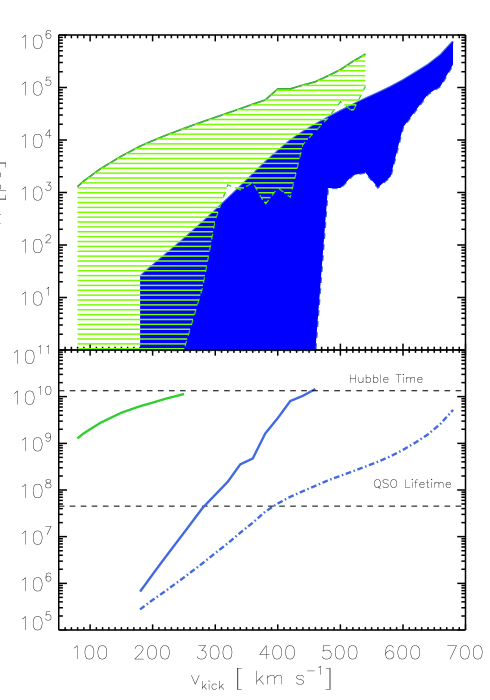
Figure 7: Upper panel: A set of apocenter distances (solid line) and pericenter distances (dashed line) for a recoiling MBH of mass $M_{\bullet}=3\times 10^{6}\,\,{\rm M_{\odot}}$ in a triaxial Milky Way-sized dark matter only host (green) and dark matter + bulge host (blue). The colored areas show the corresponding regions in the $R-V_{\rm kick}$ plane occupied by the wandering holes. Lower panel: Return timescales of a MBH in a dark matter only host (green line) and a dark matter + bulge potential (solid blue line). Also shown is the time it takes to the hole to reach its apocenter (dashed-dotted blue line).

Table 4 gives the MBH apocenter, its pericenter, and the return time calculated using our two-component model: (1) for $V_{\rm kick}>460$ $\,{\rm km\,s^{-1}}$ we stopped numerical integration after a Hubble time $t_{\rm H}$, while the hole was still wandering tens to hundreds of kiloparsecs away from the center; (2) for kick velocities below $380\,\,{\rm km\,s^{-1}}$, dynamical friction against bulge stars now efficiently damp the motion of the MBH already on the first outward trajectory, and reduces the decay timescale to less than 2 Gyr. Recoiling holes do not leave the bulge; (3) for the maximum kick velocities predicted in the case of non-rotating holes, $V_{\rm kick}\mathrel{\hbox to0.0pt{\lower 3.0pt\hbox{$\mathchar 536\relax$}\hss}\raise 2.0pt\hbox{$\mathchar 316\relax$}}200\,\,{\rm km\,s^{-1}}$, the MBH reaches a maximum distance of only 40 pc from the center and decays back within 2 Myr; (4) black holes that leave the stellar bulge and enter the triaxial dark matter halo do not return to the center within a Hubble time. The pericenter distances, apocenter distances, and the return times of MBHs are shown in Figure 7 for a dark matter only potential and a more realistic dark matter + bulge potential. According to the latter model, a MBH which is kicked with initial velocity $V_{\rm kick}=400$ $\,{\rm km\,s^{-1}}$ reaches $R_{\rm max}$ before $10^{8}$ yr, a time comparable with the typical QSO lifetime, and spends most of its time orbiting at a distance $r>1$ kpc away from the center of the bulge.

4 Summary

Coalescing MBH pairs will give origin to the loudest gravitational wave events in the universe, and are one of the primary targets for the planned Laser Interferometer Space Antenna (LISA; e.g., Sesana et al. 2004). The anisotropic emission of gravitational waves also removes net linear momentum from the binary and imparts a kick to the center of mass of the system. The outcome of this “gravitational rocket” has been the subject of many recent numerical relativity studies. Non-spinning holes recoil with velocities below 200 $\,{\rm km\,s^{-1}}$ that only depend on the binary mass ratio, while much larger kicks require rapidly rotating holes. Little is known about the masses of MBH binaries and their spins: the distribution of all binary mass ratios expected in some hierarchical models of the co-evolution of MBHs and their hosts is found to be relatively flat (Volonteri & Madau, 2008): if it is not ejected from the host altogether, the recoiling MBH will travel some maximum distance and then return towards the center on a decay timescale that depends on the shape of the potential and on the effectiveness of gas drag and dynamical friction against the stars and the dark matter of the host galaxy.

We have carried out a detailed study of the fate of bound recoling holes in Milky Way-sized potentials, running $N$-body simulations of the motion of a $M_{\rm BH}=3.7\times 10^{6}\,\,{\rm M_{\odot}}$ MBH remnant in the “Via Lactea I” dark matter halo. In the simulations, the MBH receives a kick velocity of $V_{\rm kick}$ = 80, 120, 200, 300, and 400 $\,{\rm km\,s^{-1}}$ following the coalescence of its progenitor binary, and moves within the “live” host subject only to gravity and dynamical friction against the dark matter background. We have used these calculations to build realistic semi-analytic models of the hole’s trajectory in a time-varying triaxial NFW potential, where the dynamical friction force is calculated directly from the velocity dispersion tensor, and in a two-component triaxial halo+spherical bulge model. The latter case should offer a more realistic picture of the dynamics of kicked MBHs in situations where gas drag, friction by disk stars, and the heating effect of the returning hole on the central cusp are all negligible. Our results on the trajectories of recoiling MBHs can be summarized as follows:

1. Owing to asphericities in the dark matter potential, the black hole’s orbits are highly non-radial, resulting in a significantly increased decay timescale compared to the spherical case. This is in qualitative agreement with earlier results by Vicari et al. (2007).

2. In a triaxial NFW halo return timescales to the center exceed 5 Gyr already for $V_{\rm kick}=200\,\,{\rm km\,s^{-1}}$, and are longer than the Hubble time for $V_{\rm kick}\geq 250\,\,{\rm km\,s^{-1}}$.

3. In a triaxial halo+spherical bulge potential, decay timescales are much shorter than in the bulgeless case. For kick velocities $V_{\rm kick}<380\,\,{\rm km\,s^{-1}}$, dynamical friction against bulge stars now efficiently damp the motion of the MBH already on the first outward trajectory, and reduces the decay timescale to less than 2 Gyr. For recoil velocities $V_{\rm kick}>500\,\,{\rm km\,s^{-1}}$ the MBH does not return to the center of its host within a Hubble time. Recoling black holes do not leave the bulge and remain within a few tens of parsecs from the center for $V_{\rm kick}\mathrel{\hbox to0.0pt{\lower 3.0pt\hbox{$\mathchar 536\relax$}\hss}\raise 2.0pt\hbox{$\mathchar 316\relax$}}200\,\,{\rm km\,s^{-1}}$.

A kicked MBH can retain the inner parts of its accretion disk, providing fuel for a continuing luminous phase along its trajectory. Let us assume all recoiling holes accrete at a fraction $f_{E}$ of the Eddington rate $\dot{M}_{E}=4\pi GM_{\rm BH}m_{p}/(c\sigma_{T}\epsilon)$, where $\epsilon$ is the radiative efficiency. The duration of the luminous phase depends on the amount of disk material out to the radius $R_{\rm out}\approx{GM_{\rm BH}/V_{\rm kick}^{2}}$ that is carried by the hole. In the case of an $\alpha$-disk, this is given by (Loeb 2007)

$$M_{\rm disk}\approx(1.9\times 10^{6}\,\,{\rm M_{\odot}})~{}\alpha_{-1}^{-0.8}(\epsilon_{-1}/f_{E})^{-0.6}M_{7}^{2.2}V_{3}^{-2.8},$$ (26)

where $\epsilon_{-1}\equiv\epsilon/0.1$, $M_{7}\equiv M_{\rm BH}/10^{7}\,\,{\rm M_{\odot}}$, $V_{3}\equiv V_{\rm kick}/10^{3}\,\,{\rm km\,s^{-1}}$, and $\alpha_{-1}\equiv\alpha/0.1$ is the viscosity parameter. The condition $M_{\rm disk}\leq M_{\rm BH}$ then requires

$$V_{\rm kick}\geq 550\,\,{\rm km\,s^{-1}}~{}\alpha_{-1}^{-0.28}(\epsilon_{-1}/f_{E})^{-0.21}M_{7}^{0.43}.$$ (27)

For lower kick velocities $M_{\rm disk}=M_{\rm BH}$, corresponding to an AGN lifetime of $t_{\rm QSO}=\epsilon c\sigma_{T}/(4\pi Gm_{p}f_{E})\approx 4.5\times 10^{7}\,{\rm yr}\,(\epsilon_{-1}/f_{E})$. A recoiling hole/disk system with ($M_{7},\alpha,\epsilon,f_{E},M_{\rm disk})=(1,0.1,0.1,1,M_{\rm BH})$ could then be shining for half a Gigayear as an off-center quasar over a large fraction of its “wandering” phase. Thus, cases where the recoil kick is large enough to launch the MBH into the triaxial halo are favorable for the detection of off-nuclear quasars. However, if the MBH is initially embedded in a gas-rich environment, gas drag may damp its motion significantly (Guedes et al., 2008), even for moderate kicks, lowering the detection probability. Furthermore, the spins of both black holes in a MBH binary tend to align due to torques induced by the surrounding gas, reducing the kick velocity to $v_{\rm kick}<200\,\,{\rm km\,s^{-1}}$ (Bogdanović et al., 2007). The motion of a recoiling MBH in a gas-rich merger including a stellar and dark matter component will be the subject of a subsequent paper.

Figure 1: Host halo (potential) shape parameters as a function of redshift at different ellipsoidal radii. Intermediate-to-major axis ratio $q$ (solid points), minor-to-major axis ratio $s$ (empty circles), and triaxiality parameter $T$ (insets).

Insets have the same x-axis range as the main plots.

Figure 5: Properties of the VL-I main halo at $z=0$. Left: Local density averaged over an ensemble of spheres at discrete radii from the VL-I halo center (asterisks) and best fit NFW profile (solid line). Right: Average local velocity dispersion along the principal axes of the local velocity dispersion ellipsoids as a function of radius (asterisks) and best fit velocity dispersion profile (solid line). The error bars represent the dispersion around the mean value.

Table 1: VL-I halo parameters

$a$	$\rho_{s}$	$R_{s}$	$R_{200}$	$M_{200}$	$V_{\mathrm{max}}$	$v_{\mathrm{esc}}$
	($10^{6}$ M⊙ kpc${}^{-3})$	(kpc)	(kpc)	($10^{12}$ M⊙)	(km s-1)	(km s-1)
0.393	0.16	38.0	194.3	1.03	160.53	488.5
0.423	0.21	36.7	213.1	1.13	163.7	498.2
0.465	0.41	31.3	233.8	1.19	167.9	510.9
0.507	0.54	30.8	250.9	1.22	166.7	507.3
0.549	0.72	29.7	271.5	1.31	170.4	518.4
0.591	0.99	28.1	292.5	1.43	176.4	536.7
0.633	1.40	26.2	311.8	1.54	182.6	555.8
0.675	1.87	25.1	327.4	1.61	186.4	567.2
0.762	2.40	26.0	356.6	1.76	189.2	575.6
0.877	3.54	26.2	376.2	1.77	187.0	569.0
0.901	3.67	26.7	379.2	1.77	185.6	564.8
0.950	4.51	26.2	384.9	1.77	185.9	565.5
1.000	5.33	25.8	389.3	1.77	185.1	566.2

Table 2: N-body Simulation Results

Run Name	$V_{\mathrm{kick}}$	$R_{\mathrm{max}}$	$R_{\mathrm{min}}$	$t_{\mathrm{end}}$	$R_{\mathrm{end}}$	$t_{\mathrm{return}}$
	(km s-1)	(kpc)	(kpc)	(Gyr)	(kpc)	(Gyr)
VL080	80	1.18	0.03	1.15	0.09	1.16
VL120	120	2.49	0.56	1.15	1.90	2.78
VL200	200	7.69	0.72	1.15	3.71	8.45
VL300	300	28.21	1.51	1.15	14.93	$>t_{\mathrm{H}}$
VL400	400	83.65	22.95	1.15	22.95	$>t_{\mathrm{H}}$

Table 3: Best-fit parameters to the velocity dispersion profile at $z=0$.

	A	B	C	D	m	n
	(km2 s-2)	(kpc-m)	(kpc)	(kpc-n)
$\sigma_{a}^{2}$	$2.24\times 10^{4}$	1.145	172.21	0.0026	-$4.87\times 10^{3}$	1.1132
$\sigma_{b}^{2}$	$7.16\times 10^{2}$	0.567	153.55	14.300	-$1.29\times 10^{2}$	0.1217
$\sigma_{c}^{2}$	$3.65\times 10^{2}$	0.4102	117.02	22.698	-$0.19\times 10^{2}$	0.1646

Table 4: Summary of Local Properties at $z=0$

$r$	(kpc)	1	8	25	50	100	200	400
$\bar{\rho}$	(M⊙ pc-3)	7.90$\times 10^{-2}$	6.65$\times 10^{-3}$	5.64$\times 10^{-4}$	2.80 $\times 10^{-4}$	3.35 $\times 10^{-5}$	3.65$\times 10^{-5}$	1.76 $\times 10^{-6}$
$\bar{\sigma}_{a}$	($\,{\rm km\,s^{-1}}$)	102.1	148.0	143.7	148.1	126.9	121.1	79.31
$\bar{\sigma}_{b}$	($\,{\rm km\,s^{-1}}$)	83.38	125.1	124.5	116.4	85.98	79.60	50.06
$\bar{\sigma}_{c}$	($\,{\rm km\,s^{-1}}$)	77.99	113.4	116.4	106.3	77.26	63.54	38.71
$\bar{\alpha}$	(∘)	19.82	53.19	61.45	62.30	36.57	34.79	45.19
$\bar{\beta}$	(∘)	69.17	48.28	57.47	50.43	54.81	54.66	57.69
$\bar{\gamma}$	(∘)	84.10	69.04	69.31	66.32	54.63	58.78	56.22
$\sigma(\bar{\rho})$	(M⊙ pc-3)	5.88$\times 10^{-2}$	1.67$\times 10^{-3}$	1.16$\times 10^{-3}$	9.09$\times 10^{-5}$	3.13$\times 10^{-5}$	5.37 $\times 10^{-5}$	1.26$\times 10^{-6}$
$\sigma(\bar{\sigma}_{a})$	($\,{\rm km\,s^{-1}}$)	14.27	7.253	4.468	19.15	10.48	19.58	16.61
$\sigma(\bar{\sigma}_{b})$	($\,{\rm km\,s^{-1}}$)	11.36	5.470	14.94	8.877	8.874	26.34	15.64
$\sigma(\bar{\sigma}_{c})$	($\,{\rm km\,s^{-1}}$)	10.21	2.463	10.97	9.450	11.45	29.42	13.71
$\sigma(\bar{\alpha})$	(∘)	32.56	37.80	29.52	25.96	24.41	14.58	15.43
$\sigma(\bar{\beta})$	(∘)	36.66	35.48	26.46	29.98	16.02	33.27	27.06
$\sigma(\bar{\gamma})$	(∘)	7.58	12.59	22.23	21.99	25.78	29.95	17.58

Table 5: Semi-analytic Model Results

$V_{\mathrm{kick}}$	$R_{\mathrm{max}}$	$R_{\mathrm{min}}$	$t_{\mathrm{return}}$
(km s-1)	(kpc)	(kpc)	(Gyr)
200	0.0406	0.0010	0.0016
280	0.2707	0.0010	0.0415
300	0.4512	0.0010	0.0791
360	2.2022	0.0010	0.4735
380	3.7714	0.0010	1.6275
400	6.8619	0.0010	3.4846
420	10.5830	0.0010	8.0657
440	17.9090	0.0010	10.4097
460	24.0626	0.0010	$>t_{\mathrm{H}}$
500	37.2263	1.2189	$>t_{\mathrm{H}}$
560	84.6069	1.2555	$>t_{\mathrm{H}}$
600	137.3806	17.4473	$>t_{\mathrm{H}}$
680	786.7245	276.3753	$>t_{\mathrm{H}}$

References

- Allgood et al. (2006) Allgood, B., Flores, A. R., Primack, J. R., Kravtsov, A. V., Wechsler, R. H., Faltenbacher, A., & Bullock, J. S. 2006, MNRAS, 367, 1781
- Baker et al. (2008) Baker, J. G., Boggs, W. D., Centrella, J., Kelly, B. J., McWilliams, S. T., Miller, M. C., & van Meter, J. R. 2008, ApJ, 682, L29
- Baker et al. (2006a) Baker, J. G., Centrella, J., Choi, D.-I., Koppitz, M., & van Meter, J. 2006a, PhysRevL, 96, 111102
- Baker et al. (2006b) Baker, J. G., Centrella, J., Choi, D.-I., Koppitz, M., van Meter, J. R., & Miller, M. C. 2006b, ApJ, 653, L93
- Begelman et al. (1980) Begelman, M. C., Blandford, R. D., & Rees, M. J. 1980, Nature, 287, 307
- Bekenstein (1973) Bekenstein, J. D. 1973, ApJ, 183, 657]
- Bertschinger (2001) Bertschinger, E. 2001, ApJS, 137,1B
- Binney & Tremaine (1987) Binney, J., & Tremaine, S. 1987, Galactic Dynamics (Princeton: Princeton Univ. Press)
- Blecha & Loeb (2008) Blecha, L., & Loeb, A. 2008, MNRAS, 390, 1311
- Bogdanović et al. (2009) Bogdanović, T., Eracleous, M.; Sigurdsson, S. 2009, ApJ, 697, 288
- Bogdanović et al. (2007) Bogdanović, T., Reynolds, C. S., & Miller, C. 2007, ApJ, 661, L147
- Bonning, Shields, & Salviander (2007) Bonning, E. W., Shields, G. A., & Salviander, S. 2007, ApJ, 666, L13
- Boylan-Kolchin et al. (2004) Boylan-Kolchin, M., Ma, C.-P., & Quataert, E. 2004, ApJ, 613, L37
- Campanelli et al. (2006) Campanelli, M., Lousto, C. O., Marronetti, P., & Zlochower, Y. 2006, Phys. Rev. Lett., 96, 111101
- Campanelli et al. (2007a) Campanelli, M., Lousto C., Zlochower, Y., & Merrit, D. 2007, ApJ, 659, L5
- Chandrasekhar (1943) Chandrasekhar, S. 1943, ApJ, 97, 255
- Colpi et al. (1999) Colpi M. , Mayer L., & Governato F. 1999, ApJ, 525, 720
- Diemand et al. (2007a) Diemand J., Kuhlen M., & Madau P. 2007a, ApJ, 657, 262
- Diemand et al. (2007b) Diemand J., Kuhlen M., & Madau P. 2007b, ApJ, 671, 1135
- Diemand et al. (2008) Diemand, J., Kuhlen, M., Madau, P., Zemp, M., Moore, B., Potter, D., & Stadel, J. 2008, Nature, 454, 735
- Dotti et al. (2008) Dotti, M., Montuori, C., Decarli, R., Volonteri, M., Colpi, M., & Haardt, F. 2008, arXiv:astro-ph/ 0809.3446
- Favata et al. (2004) Favata, M., Hughes, S.A., & Holz, D.E. 2004, ApJ, 607, L5
- Fitchett & Detweiler (1984) Fitchett, M.J. & Detweiler, S. 1984, MNRAS, 211, 933
- Franx et al. (1991) Franx, M., Illingworth, G., & de Zeeuw, T. 1991, ApJ, 383, 112
- Ghez et al. (2005) Ghez, A. M., Salim, S., Hornstein, S. D., Tanner, A., Lu, J. R., Morris, M., Becklin E. E., & Duchêne, G. 2005, ApJ, 620, 744
- González et al. (2007) González, J. A., Hannam, M., Sperhake, U., Brügmann, B., & Husa, S. 2007, Phys. Rev. Lett., 98, 231101
- Gualandris & Merritt (2008) Gualandris, A., & Merritt, D. 2008, ApJ, 678, 780
- Guedes et al. (2008) Guedes, J., Diemand, J., Zemp, M., Kuhlen, M., Madau, P., Mayer, L., & Stadel, J. 2008, Astron. Naschr., 329, 1004
- Hashimoto et al. (2003) Hashimoto, Y., Funato, Y., & Makino, J. 2003, ApJ, 582, 196
- Heckman et al. (2009) Heckman, T., Krolik, J. H., Moran, S. M., Schnittman, J., & Gezari, S. 2009, ApJ, 695, 363
- Herrmann et al. (2007) Herrmann, F., Hinder, I., Shoemaker, D., & Laguna, P. 2007, Class. Quantum Grav., 24, 33
- Komossa et al. (2003) Komossa, S., Burwitz, V., Hasinger, G., Predehl, P., Kaastra, J. S., & Ikebe, Y. 2003, ApJ, 582, L15
- Komossa et al. (2008) Komossa, S., Zhou, & H., Lu, H. 2008, ApJ, 678, 81
- Kormendy et al. (1995) Kormendy, J. & Richtsone, D. 1995, ARA&A, 30, 581
- Kuhlen et al. (2007) Kuhlen, M., Diemand, J., & Madau, P. 2007, ApJ, 671, 1135
- Loeb (2007) Loeb, A. 2007 Phys. Rev. Lett., 99, 041103
- Madau & Quataert (2004) Madau, P. & Quataert, E. 2004, ApJ, 606, L17
- Madau & Rees (2001) Madau P. & Rees, M. J. 2001, ApJ, 551, L27
- Maoz (1993) Maoz, E. 1993, MNRAS, 263, 75
- Max et al. (2007) Max, C., E., Canalizo, G., & de Vries, W. H. 2007, Science, 316, 1877
- Mayer et al. (2007) Mayer, L., Kazantzidis, S., Madau, P., Colpi, M., Quinn, T., & Wadsley, J. 2007, Science, 316, 1874
- Navarro et al. (1997) Navarro, J. F., Frenk, C. S., & White, S. D. M. 1997, ApJ, 490, 493
- Pesce et al. (1992) Pesce, E., Capuzzo-Dolcetta, R., & Vietri M. 1992, MNRAS, 254, 466
- Pretorius (2005) Pretorius, F. 2005, Phys. Rev. Lett., 95, 121101
- Richtsone et al. (1998) Richtsone, D., et al. 1998, Nature, 395, A14
- Rodriguez et al. (2006) Rodriguez, C., Taylor, G. B., Zavala, R. T., Peck, A. B., Pollack, L. K., & Romani, R. W. 2006, ApJ, 646, 49
- Sesana et al. (2004) Sesana, A., Haardt, F., Madau, P., & Volonteri, M. 2004, ApJ, 611, 623
- Shields et al. (2009) Shields, G. A.; Bonning, E. W.; Salviander, S. 2009, ApJ, 696, 1367
- Spergel et. al (2007) Spergel, D. N., et al. 2007, ApJS, 170, 377
- Stadel (2001) Stadel, J. 2001, PhD thesis, University of Washington
- Stadel et al. (2008) Stadel, J., Potter, D., Moore, B., Diemand, J., Kuhlen, M., Madau, P., Zemp, M., & Quilis, V. 2008, MNRAS, submitted (arXiv:astro-ph/0808.2981)
- Tanaka & Haiman (2009) Tanaka, T., & Haiman, Z. 2009, ApJ, 696,1798
- Tremaine et al. (2002) Tremaine, S., et al. 2002, ApJ, 574, 740
- Vicari et al. (2007) Vicari, A., Capuzzo-Dolcetta, R., & Merritt, D. 2007, ApJ, 662, 797
- Volonteri et al. (2003) Volonteri, M., Haardt, F., & Madau, P. 2003, ApJ, 582, 559
- Volonteri & Madau (2008) Volonteri, M., & Madau, P. 2008, ApJ, 687, L57
- Volonteri & Rees (2006) Volonteri, M., & Rees, M. 2006, ApJ, 650,669
- Zemp et al. (2009) Zemp, M., Diemand, J., Kuhlen, M., Madau, P., Moore, B., Potter, D., Stadel, J., & Widrow, L. 2009, MNRAS, 394,641
- Zentner & Bullock (2003) Zentner, A., & Bullock, J. 2003, ApJ, 598, 49