Self-Improving Algorithms††thanks: Preliminary versions appeared as N. Ailon, B. Chazelle, S. Comandur, and D. Liu, Self-improving Algorithms in Proc. 17th SODA, pp. 261–270, 2006; and K. L. Clarkson and C. Seshadhri, Self-improving Algorithms for Delaunay Triangulations in Proc. 24th SoCG, pp. 148–155, 2008. This work was supported in part by NSF grants CCR-998817, 0306283, ARO Grant DAAH04-96-1-0181.
Abstract
We investigate ways in which an algorithm can improve its expected performance by fine-tuning itself automatically with respect to an unknown input distribution . We assume here that is of product type. More precisely, suppose that we need to process a sequence of inputs of some fixed length , where each is drawn independently from some arbitrary, unknown distribution . The goal is to design an algorithm for these inputs so that eventually the expected running time will be optimal for the input distribution .
We give such self-improving algorithms for two problems: (i) sorting a sequence of numbers and (ii) computing the Delaunay triangulation of a planar point set. Both algorithms achieve optimal expected limiting complexity. The algorithms begin with a training phase during which they collect information about the input distribution, followed by a stationary regime in which the algorithms settle to their optimized incarnations.
keywords:
average case analysis, Delaunay triangulation, low entropy, sortingAMS:
68Q25, 68W20, 68W401 Introduction
The classical approach to analyzing algorithms draws a familiar litany of complaints: worst-case bounds are too pessimistic in practice, say the critics, while average-case complexity too often rests on unrealistic assumptions. The charges are not without merit. Hard as it is to argue that the only permutations we ever want to sort are random, it is a different level of implausibility altogether to pretend that the sites of a Voronoi diagram should always follow a Poisson process or that ray tracing in a BSP tree should be spawned by a Gaussian. Efforts have been made to analyze algorithms under more complex models (eg, Gaussian mixtures, Markov model outputs) but with limited success and lingering doubts about the choice of priors.
Suppose we wish to compute a function that takes as input. We get a sequence of inputs , and wish to compute , . It is quite plausible to assume that all these inputs are somehow related to each other. This relationship, though exploitable, may be very difficult to express concisely. One way of modeling this situation is to postulate a fixed (but complicated) unknown distribution of inputs. Each input is chosen independently at random from . Is it possible to learn quickly something about so that we can compute ( chosen from ) faster? (Naturally, this is by no means the only possible input model. For example, we could have a memoryless Markov source, where each depends only on . However, for simplicity we will here focus on a fixed source that generates the inputs independently.)
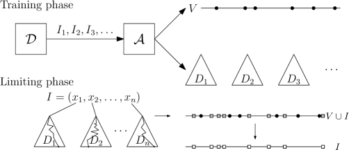
That is what a self-improving algorithm attempts to do. Initially, since nothing is know about , our self-improving algorithm can only provide some worst-case guarantee. As the algorithm sees more and more inputs, it can learn something about the structure of . We call this the training phase of the self-improving algorithm. During this phase, the algorithm collects and organizes information about the inputs in the hope that it can be used to improve the running time (with respect to inputs from . The algorithm then moves to the limiting phase. Having decided that enough has been learned about , the algorithm uses this information to compute faster. Note that this behavior is tuned to the distribution .

Obviously, there is no reason why we should get a faster running time for all . Indeed, if is the sorting function and is the uniform distribution over permutations, then we require expected time to sort. On the other hand, if was a low-entropy source of inputs, it is quite reasonable to hope for a faster algorithm. So when can we improve our running time? An elegant way of expressing this is to associate (using information theory) an “optimal” running time for each distribution. This is a sort of estimate of the best expected running time we can hope for, given inputs chosen from a fixed distribution . Naturally, the lower the entropy of , the lower this running time will be. In the limiting phase, our self-improving algorithm should achieve this optimal running time.
To expect a good self-improving algorithm that can handle all distributions seems a bit ambitious, and indeed we show that even for the sorting problem there can be no space-efficient such algorithm (even when the entropy is low). Hence, it seems necessary to impose some kind of restriction on . However, if we required to be, say, uniform or a Gaussian, we would again be stuck with the drawbacks of traditional average case analysis. Hence, for self-improvement to be of any interest, the restricted class of distributions should still be fairly general. One such class is given by product distributions.
1.1 Model and Results
We will focus our attention on distributions of product type. Think of each input as an -dimensional vector over some appropriate domain. This could be a list of numbers (in the case of sorting) or a list of points (for Delaunay triangulations). Each is generated independently at random from an arbitrary distribution , so . All the ’s are independent of each other. It is fairly natural to think of various portions of the input as being generated by independent sources. For example, in computational geometry, the convex hull of uniformly independently distributed points in the unit square is a well studied problem.
Note that all our inputs are of the same size . This might appear to be a rather unnatural requirement for (say) a sorting algorithm. Why must the 10th number in our input come from the same distribution? We argue that this is not a major issue (for concreteness, let us focus on sorting). The right way to think of the input is as a set of sources , each independently generating a single number. The actual “order” in which we get these numbers is not important. What is important is that for each number, we know its source. For a given input, it is realistic to suppose that some sources may be active, and some may not (so the input may have less than numbers). Our self-improving sorters essentially perform an independent processing on each input number, after which time is enough to sort.111The self-improving Delaunay triangulation algorithms have a similar behavior. The algorithm is completely unaffected by the inactive sources. To complete the training phase, we only need to get enough information about each source. What if new sources are introduced during the stationary phase? Note that as long as new sources (and hence new numbers) are added, we can always include these extra numbers in the sorted list in time. Once the number of new sources becomes too large, we will have to go back to the training phase. This is, of course, quite acceptable: if the underlying distribution of inputs changes significantly, we have to recalibrate the algorithm. For these reasons, we feel that it is no loss of generality to deal with a fixed input length, especially for product distributions.
Our first result is a self-improving sorter. Given a source of real-number sequences , let denote the permutation induced by the ranks of the ’s, using the indices to break ties. Observe that since is a random variable, so is . We can define the entropy , over the randomness of , and the limiting complexity of our algorithm will depend on . Note this quantity may be much smaller than the entropy of the source itself but can never exceed it.
As we mentioned earlier, the self-improving algorithm initially undergoes a training phase. At the end of this phase, some data structures storing information about the distributions are constructed. In the limiting phase, the self-improving algorithm is fixed, and these data structures do not change. In the context of sorting, the self-improving sorter becomes some fixed comparison tree.
Theorem 1.
There exists a self-improving sorter of limiting complexity, for any input distribution . Its worst case running time is . No comparison-based algorithm can sort an input from in less than time. For any constant , the storage can be made for an expected running time of . The training phase lasts rounds and the probability that it fails is at most .
Why do we need a restriction on the input distribution? In §3.3, we show that a self-improving sorter that can handle any distribution requires an exponentially large data structure. Fredman [31] gave an algorithm that could optimally sort permutations from any distribution . His algorithm needs to know explicitly, and it constructs lookup tables of exponential size. Our bound shows that Fredman’s algorithm cannot be improved. Furthermore, we show that even for product distributions any self-improving sorter needs super-linear space. Hence, our time-space tradeoffs are essentially optimal. We remind the reader that we focus on comparison-based algorithms.
Theorem 2.
Consider a self-improving algorithm that, given any fixed distribution , can sort a random input from in expected time. Such an algorithm requires bits of storage.
Let . Consider a self-improving algorithm that, given any product distribution , can sort a random input from in expected time. Such an algorithm requires a data structure of bit size .
For our second result, we take the notion of self-improving algorithms to the geometric realm and address the classical problem of computing the Delaunay triangulation of a set of points in the Euclidean plane. Given a source of sequences of points in , let denote the Delaunay triangulation of . If we interpret as a random variable on the set of all undirected graphs with vertex set , then has an entropy , and the limiting complexity of our algorithm depends on this entropy.
Theorem 3.
There exists a self-improving algorithm for planar Delaunay triangulations of limiting complexity, for any input distribution . Its worst case running time is . For any constant , the storage can be made for an expected running time of . The training phase lasts rounds and the probability that it fails is at most .
From the linear time reduction from sorting to computing Delaunay triangulations [14, Theorems 8.2.2 and 12.1.1], the lower bounds of Theorem 2 carry over to Delaunay triangulations.
Both our algorithms follow the same basic strategy. During the training phase, we collect data about the inputs in order to obtain a typical input instance for with , and we compute the desired structure (a sorted list or a Delaunay triangulation) on . Then for each distribution , we construct an entropy optimal search structure for (ie, an entropy optimal binary search tree or a distribution sensitive planar point location structure). In the limiting phase, we use the ’s in order to locate the components of a given input in . The fact that is a typical input ensures that will be broken into individual subproblems of expected constant size that can be solved separately, so we can obtain the desired structure for the input in expected linear time (plus the time for the -searches). Finally, for both sorting and Delaunay triangulation it suffices to know the solution for in order to derive the solution for in linear expected time [21, 22]. Thus, the running time of our algorithms is dominated by the -searches, and the heart of the analysis lies in relating this search time to the entropies and , respectively.
1.2 Previous Work
Related concepts to self-improving algorithms have been studied before. List accessing algorithms and splay trees are textbook examples of how simple updating rules can speed up searching with respect to an adversarial request sequence [45, 46, 5, 15, 35]. It is interesting to note that self-organizing data structures were investigated over stochastic input models first [4, 6, 13, 32, 40, 44]. It was the observation [11] that memoryless sources for list accessing are not terribly realistic that partly motivated work on the adversarial models. It is highly plausible that both approaches are superseded by more sophisticated stochastic models: for example, hidden Markov models for gene finding or speech recognition or time-coherent models for self-customized BSP trees [8] or for randomized incremental constructions [23]. Recently, Afshani et al. [1] introduced the notion of instance optimality, which can be seen as a generalization of output-sensitivity. They consider the inputs as sets and try to exploit the structure within each input for faster algorithms.
Much research has been done on adaptive sorting [30], especially on algorithms that exploit near-sortedness. Our approach is conceptually different: we seek to exploit properties, not of individual inputs, but of their distribution. Algorithmic self-improvement differs from past work on self-organizing data structures and online computation in two fundamental ways. First, there is no notion of an adversary: the inputs are generated by a fixed, oblivious, random source , and we compare ourselves against an optimal comparison-based algorithm for . In particular, there is no concept of competitiveness. Second, self-improving algorithms do not exploit structure within any given input but, rather, within the ensemble of input distributions.
A simple example highlights this difference between previous sorters and the self-improving versions. For , fix two random integers from . The distribution is such that , and we take . Observe that every permutation generated by is a random permutation, since the ’s and ’s are chosen randomly. Hence, any solution in the adaptive, self-organizing/adjusting framework requires time, because no input exhibits any special structure to be exploited. On the other hand, our self-improving sorter will sort a permutation from in expected linear time during the limiting phase: since generates at most different permutations, we have .
2 Entropy and Comparison-based Algorithms
Before we consider sorting and Delaunay triangulations, let us first recall some useful properties of information theoretic entropy [28] and explain how it relates to our notion of comparison-based algorithms.
Let be a random variable with a finite range . The entropy of , , is defined as . Intuitively, the event that gives us bits of information about the underlying elementary event, and represents the expected amount of information that can be obtained from observing . We recall the following well-known property of the entropy of the Cartesian product of independent random variables [28, Theorem 2.5.1].
Claim 4.
Let be the joint entropy of independent random variables . Then
We now define our notion of a comparison-based algorithm. Let be an arbitrary universe, and let be a finite set. A comparison-based algorithm to compute a function is a rooted binary tree such that (i) every internal node of represents a comparison of the form , where are arbitrary functions on the input universe ; and (ii) the leaves of are labeled with outputs from such that for every input , following the appropriate path for leads to the correct output . If has maximum depth , we say that needs comparisons (in the worst case). For a distribution on , the expected number of comparisons (with respect to ) is the expected length of a path from the root to a leaf in , where the leaves are sampled according to the distribution that induces on via .
Note that our comparison-based algorithms generalize both the traditional notion of comparison-based algorithms [27, Chapter 8.1], where the functions and are required to be projections, as well as the notion of algebraic computation trees [9, Chapter 16.2]. Here the functions and must be composed of elementary functions (addition, multiplication, square root) such that the complexity of the composition is proportional to the depth of the node. Naturally, our comparison-based algorithms can be much stronger. For example, deciding whether a sequence of real numbers consists of distinct elements needs one comparison in our model, whereas every algebraic computation tree for the problem has depth [9, Chapter 16.2]. However, for our problems of interest, we can still derive meaningful lower bounds.
Claim 5.
Let be a distribution on a universe and let be a random variable. Then any comparison-based algorithm to compute needs at least expected comparisons.
Proof.
This is an immediate consequence of Shannon’s noiseless coding theorem [28, Theorem 5.4.1] which states that any binary encoding of an information source such as must have an expected code length of at least . Any comparison-based algorithm represents a coding scheme: the encoder sends the sequence of comparison outcomes, and the decoder descends along the tree , using the transmitted sequence to determine comparison outcomes. Thus, any comparison-based algorithm must perform at least comparisons in expectation. ∎
Note that our comparison-based algorithms include all the traditional sorting algorithms [27] (selection sort, insertion sort, quicksort, etc) as well as classic algorithms for Delaunay triangulations [12] (randomized incremental construction, divide and conquer, plane sweep). A notable exception are sorting algorithms that rely on table lookup or the special structure of the input values (such as bucket sort or radix sort) as well as transdichotomous algorithms for sorting [33, 34] or Delaunay triangulations [16, 17, 18].
The following lemma shows how we can use the running times of comparison-based algorithms to relate the entropy of different random variables. This is a very important tool that will be used to prove the optimality of our algorithms.
Lemma 6.
Let be a distribution on a universe , and let and be two random variables. Suppose that the function defined by can be computed by a comparison-based algorithm with expected comparisons (where the expectation is over ). Then , where all the entropies are with respect to .
Proof.
Let be a unique binary encoding of . By unique encoding, we mean that the encoding is . We denote the expected code length of with respect to , , by . By another application of Shannon’s noiseless coding theorem [28, Theorem 5.4.1]), we have for any unique encoding of , and there exists a unique encoding of with .
Using , we can convert into a unique encoding of . Indeed, for every , can be uniquely identified by a string that is the concatenation of and additional bits that represent the outcomes of the comparisons for the algorithm to compute . Thus, for every element , we can define as the lexicographically smallest string for which , and we obtain a unique encoding for . For the expected code length of , we get
Since Shannon’s theorem implies , the claim follows. ∎
3 A Self-Improving Sorter
We are now ready to describe our self-improving sorter. The algorithm takes an input of real numbers drawn from a distribution (ie, each is chosen independently from ). Let denote the permutation induced by the ranks of the ’s, using the indices to break ties. By applying Claim 5 with , the set of all permutations on , and , we see that any sorter must make at least expected comparisons. Since it takes steps to write the output, any sorter needs steps. This is, indeed, the bound that our self-improving sorter achieves.
For simplicity, we begin with the steady-state algorithm and discuss the training phase later. We also assume that the distribution is known ahead of time and that we are allowed some amount of preprocessing before having to deal with the first input instance (§3.1). Both assumptions are unrealistic, so we show how to remove them to produce a bona fide self-improving sorter (§3.2). The surprise is how strikingly little of the distribution needs to be learned for effective self-improvement.
3.1 Sorting with Full Knowledge
We consider the problem of sorting , where each is a real number drawn from a distribution . We can assume without loss of generality that all the ’s are distinct. (If not, simply replace by for an infinitesimally small , so that ties are broken according to the index .)
The first step of the self-improving sorter is to sample a few times (the training phase) and create a “typical” instance to divide the real line into a set of disjoint, sorted intervals. Next, given some input , the algorithm sorts by using the typical instance, placing each input number in its respective interval. All numbers falling into the same intervals are then sorted in a standard fashion. The algorithm needs a few supporting data structures.
-
•
The -list: Fix an integer parameter , and sample input instances from . Form their union and sort the resulting -element multiset into a single list . Next, extract from it every -th item and form the list , where , , and for . Keep the resulting -list in a sorted table as a snapshot of a “typical” input instance. We will prove the remarkable fact that, with high probability, locating each in the -list is linearly equivalent to sorting . We cannot afford to search the -list directly, however. To do that, we need auxiliary search structures.
-
•
The -trees: For any , let be the predecessor222Throughout this paper, the predecessor of in a list refers to the index of the largest list element ; it does not refer to the element itself. of a random from in the -list, and let be the entropy of . The -tree is defined to be an optimum binary search tree [41] over the keys of the -list, where the access probability of is , for any . This allows us to compute using expected comparisons.
The self-improving sorter. The input is sorted by a two-phase procedure. First we locate each in the -list using the -trees. This allows us to partition into groups of ’s sharing the same predecessor in the -list. The first phase of the algorithm takes expected time.333The ’s themselves are random variables depending on the choice of the -list. Therefore, this is a conditional expectation. The next phase involves going through each and sorting their elements naively, say using insertion sort, in total time . See Fig. 2.
The expected running time is , and the total space used is . This can be decreased to for any constant ; we describe how at the end of this section. First, we show how to bound the running time of the first phase. This is where we really show the optimality of our sorter.
Lemma 7.
Proof.
Our proof actually applies to any linear sized sorted list . Let be the sequence of predecessors for all elements in . By Claim 4, we have , so it suffices to bound the entropy of . By Lemma 6 applied with , and , it suffices to give a comparison-based algorithm that can determine from with comparisons. But this is easy: just use to sort (which needs no further comparisons) and then merge the sorted list with . Now the lemma follows from Claim 4. ∎
Next we deal with the running time of the second phase. As long as the groups are small, the time to sort each group will be small. The properties of the -list ensure that this is the case.
Lemma 8.
For , let be the elements with predecessor . With probability at least over the construction of the -list, we have and , for all .
Proof.
Remember that the -list was formed by taking certain elements from a sequence that was obtained by concatenating inputs , , . Let be any two elements from , and let . Note that all the other numbers are independent of and . Suppose we fix the values of and (in other words, we condition on the values of and ). For every , let be the indicator random variable for the event that , and let . Since all the ’s are independent, by Chernoff’s bound [42, Theorem 4.2], for any ,
| (1) |
Setting , we see that if , then with probability at least . Note that this is true for every fixing of and . Therefore, we get the above statement even with the unconditioned random variable . Now, by applying the same argument to any pair with and taking a union bound over all such pairs, we get that with probability at least over the construction of the following holds for all half-open intervals defined by pairs with : if , then . From now on we assume that this implication holds.
The -list is constructed such that for , , and hence . Let be the indicator random variable for the event that lies in , and . Note that (where and denote the indices of and in )
and therefore . Now, since the expectation of is constant, and since is a sum of independent indicator random variables, we can apply the following standard claim in order to show that the second moment of is also constant.
Claim 9.
Let be a sum of independent positive random variables with for all and . Then .
Combining Lemmas 7 and 8, we get the running time of our self-improving sorter to be . This proves the optimality of time taken by the sorter.
We now show that the storage can be reduced to , for any constant . The main idea is to prune each -tree to depth . This ensures that tree has size , so the total storage used is . We also construct a completely balanced binary tree for searching in the -list. Now, when we wish to search for in the -list, we first search using the pruned -tree. At the end, if we reach a leaf of the unpruned -tree, we stop since we have found the right interval of the -list which contains . On the other hand, if the search in the -tree was unsuccessful, then we use for searching.
In the first case, the time taken for searching is simply the same as with unpruned -trees. In the second case, the time taken is . But note that the time taken with unpruned -trees is at least (since the search on the pruned -tree failed, we must have reached some internal node of the unpruned tree). Therefore, the extra time taken is only a factor of the original time. As a result, the space can be reduced to with only a constant factor increase in running time (for any fixed ).
3.2 Learning the Distribution
In the last section we showed how to obtain a self-improving sorter if is known. We now explain how to remove this assumption. The -list is built in the first rounds, as before. The -trees will be built after additional rounds, which will complete the training phase. During that phase, sorting is handled via, say, mergesort to guarantee complexity. The training part per se consists of learning basic information about for each . For notational simplicity, fix and let . Let , for a large enough constant . For any , let be the number of times, over the first rounds, that is found to be the -list predecessor of . (We use standard binary search to compute predecessors in the training phase.) Finally, define the -tree to be a weighted binary search tree defined over all the ’s such that . Recall that the crucial property of such a tree is that the node associated with a key of weight is at depth . We apply this procedure for each .
This -tree is essentially the pruned version of the tree we used in §4.1. Like before, its size is , and it is used in a similar way as in §4.1, with a few minor differences. For completeness, we go over it again: given , we perform a search down the -tree. If we encounter a node whose associated key is such that , we have determined and we stop the search. If we reach a leaf of the -tree without success, we simply perform a standard binary search in the -list.
Lemma 10.
Fix . With probability at least , for any , if then .
Proof.
The expected value of is . If then, by Chernoff’s bound [7, Corollary A.17] the count deviates from its expectation by more than with probability less than (recall that )
for large enough. A union bound over all completes the proof. ∎
Suppose now the implication of Lemma 10 holds for all (and fixed ). We show now that the expected search time for is . Consider each element in the sum . We distinguish two cases.
- •
-
•
Case 2: . The search time is always ; hence the contribution to the expected search time is .
By summing up over all , we find that the expected search time is . This assumes the implication of Lemma 10 for all . By a union bound, this holds with probability at least . The training phase fails when either this does not hold, or if the -list does not have the desired properties (Lemma 8). The total probability of this is at most .
3.3 Lower Bounds
Can we hope for a result similar to Theorem 1 if we drop the independence assumption? The short answer is no. As we mentioned earlier, Fredman [31] gave a comparison-based algorithm that can optimally sort any distribution of permutations. This uses an exponentially large data structure to decide which comparisons to perform. Our lower bound shows that the storage used by Fredman’s algorithm is essentially optimal.
To understand the lower bound, let us try to abstract out the behavior of a self-improving sorter. Given inputs from a distribution , at each round, the self-improving sorter is just a comparison tree for sorting. After any round, the self-improving sorter may wish to update the comparison tree. At some round (eventually), the self-improving sorter must be able to sort with expected comparisons: the algorithm has “converged” to the optimal comparison tree. The algorithm uses some data structure to represent (implicitly) this comparison tree.
We can think of a more general situation. The algorithm is explicitly given an input distribution . It is allowed some space where it stores information about (we do not care about the time spent to do this). Then, (using this stored information) it must be able to sort a permutation from in expected comparisons. So the information encodes some fixed comparison based procedure. As a shorthand for the above, we will say that the algorithm, on input distribution , optimally sorts . How much space is required to deal with all possible ’s? Or just to deal with product distributions? These are the questions that we shall answer.
Lemma 11.
Let , for some sufficiently large constant , and let be an algorithm that can optimally sort any input distribution with . Then requires bits of storage.
Proof.
Consider the set of all permutations of . Every subset of permutations induces a distribution defined by picking every permutation in with equal probability and none other. Note that the total number such distributions is and , where is the distribution on the output induced by . Suppose there exists a comparison-based procedure that sorts a random input from in expected time at most , for some constant . By Markov’s inequality this implies that at least half of the permutations in are sorted by in at most comparisons. But, within comparisons, the procedure can only sort a set of at most permutations. Therefore, any other such that will have to draw at least half of its elements from . This limits the number of such to
This means that the number of distinct procedures needed exceeds
assuming that is small enough. A procedure is entirely specified by a string of bits; therefore at least one such procedure must require storage logarithmic in the previous bound. ∎
We now show that a self-improving sorter dealing with product distributions requires super-linear size. In fact, the achieved tradeoff between the storage bound and an expected running time off the optimal by a factor of is optimal.
Lemma 12.
Let be a large enough parameter, and let be an algorithm that, given a product distribution , can sort a random permutation from in expected time . Then requires a data structure of bit size .
Proof.
The proof is a specialization of the argument used for proving Lemma 11. Let and . We define by choosing distinct integers in and making them equally likely to be picked as . (For convenience, we use the tie-breaking rule that maps . This ensures that is unique.) We then set . By Claim 4, has entropy . This leads to choices of distinct distributions . Suppose that uses bits of storage and can sort each such distribution in expected comparisons. Some fixing of the bits must be able to accommodate this running time for a set of at least distributions . In other words, some comparison-based procedure can deal with distributions . Any input instance that is sorted in at most time by is called easy: the set of easy instances is denoted by .
Because has to deal with many distributions, there must be many instances that are easy for . This gives a lower bound for . On the other hand, since easy instances are those that are sorted extremely quickly by , there cannot be too many of them. This gives an upper bound for . Combining these two bounds, we get a lower bound for . We will begin with the easier part: the upper bound for .
Claim 13.
Proof: In the comparison-based algorithm represented by , each instance is associated with a leaf of a binary decision tree of depth at most , ie, with one of at most leaves. This would give us an upper bound on if each was assigned a distinct leaf. However, it may well be that two distinct inputs have and lead to the same leaf. Nonetheless, we have a collision bound, saying that for any permutation , there are at most instances with . This implies that .
To prove the collision bound, first fix a permutation . How many instances can map to this permutation? We argue that knowing that for an instance , we only need additional bits to encode . This immediately shows that there must be less than such instances . Write , and let be sorted to give the vector . Represent the ground set of as an -bit vector ( if some , else ). For , let if , else . Now, given and , we can immediately deduce the vector , and by applying to , we get . This proves the collision bound. ∎
Claim 14.
Proof: Each is characterized by a vector , so that itself is specified by . (From now on, we view both as a vector and a distribution of input instances.) Define the -th projection of as . Even if , it could well be that none of the projections of are easy. However, if we consider the projections obtained by permuting the coordinates of each vector in all possible ways we enumerate each input instance from the same number of times. Note that applying these permutations gives us different vectors which also represent . Since the expected time to sort an input chosen from is at most , by Markov’s inequality, there exists a choice of permutations (one for each ) for which at least half of the projections of the vector obtained by applying these permutations are easy.
Let us count how many distributions have a vector representation with a choice of permutations placing half its projections in . There are fewer than choices of such instances and, for any such choice, each has half its entries already specified, so the remaining choices are fewer than . This gives an upper bound of on the number of such distributions. This number cannot be smaller than ; therefore , as desired.
It now just remains to put the bounds together.
We have and . Since is sufficiently large, we get .
4 Delaunay Triangulations
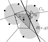
We now consider self-improving algorithms for Delaunay triangulations. The aim of this section is to prove Theorem 3. Let denote an input instance, where each is a point in the plane, generated by a point distribution . The distributions are arbitrary, and may be continuous, although we never explicitly use such a condition. Each is independent of the others, so in each round the input is drawn from the product distribution , and we wish to compute the Delaunay triangulation of , . To keep our arguments simple, we will assume that the points of are in general position (ie, no four points in lie on a common circle). This is no loss of generality and does not restrict the distribution , because the general position assumption can always be enforced by standard symbolic perturbation techniques [29]. Also we will assume that there is a bounding triangle that always contains all the points in . Again, this does not restrict the distribution in any way, because we can always simulate the bounding triangle symbolically by adding virtual points at infinity.
The distribution induces a (discrete) distribution on the set of Delaunay triangulations, viewed as undirected graphs with vertex set . Consider the entropy of this distribution: for each graph on , let be the probability that it represents the Delaunay triangulation of . We have the output entropy . By Claim 5, any comparison-based algorithm to compute the Delaunay triangulation of needs at least expected comparisons. Hence, an optimal algorithm will be one that has an expected running time of (since it takes steps to write the output).
We begin by describing the basic self-improving algorithm. (As before, we shall first assume that some aspects of the distribution are known.) Then, we shall analyze the running time using our information theory tools to argue that the expected running time is optimal. Finally, we remove the assumption that is known and give the time-space tradeoff in Theorem 3.
4.1 The algorithm
We describe the algorithm in two parts. The first part explains the learning phase and the data structures that are constructed (§4.1.1). Then, we explain how these data structures are used to speed up the computation in the limiting phase (§4.1.2). As before, the expected running time will be expressed in terms of certain parameters of the data structures obtained in the learning phase. In the next section (§4.2), we will prove that these parameters are comparable to the output entropy . First, we will assume that the distributions are known to us, and the data structures described will use space. Section 4.3 repeats the arguments of §3.2 to remove this assumption and to give the space-time tradeoff bounds of Theorem 3.
As outlined in Fig. 3, our algorithm for Delaunay triangulation is roughly a generalization of our algorithm for sorting. This is not surprising, but note that while the steps of the two algorithms, and their analyses, are analogous, in several cases a step for sorting is trivial, but the corresponding step for Delaunay triangulation uses some relatively recent and sophisticated prior work.
| Sorting | Delaunay Triangulation |
|---|---|
| Intervals containing no values of | Delaunay disks |
| Typical set | Range space -net [39, 26], ranges are disks, |
| training instance points with the same value | training instance points in each Delaunay disk |
| Expect values of within each bucket (of the same index) | Expect points of in each Delaunay disk of |
| Optimal weighted binary trees | Entropy-optimal planar point location data structures [10] |
| Sorting within buckets | Triangulation within (Claim 19) |
| Sorted list of | |
| Build sorted from sorted (trivial) | Build from [21, 22] |
| (analysis) merge sorted and | (analysis) merge and [19] |
| (analysis) recover the indices from the sorted (trivial) | (analysis) recover the triangles in from (Lemma 22) |
4.1.1 Learning Phase
For each round in the learning phase, we use a standard algorithm to compute the output Delaunay triangulation. We also perform some extra computation to build some data structures that will allow speedup in the limiting phase.
The learning phase is as follows. Take the first input lists , , , . Merge them into one list of points. Setting , find an -net for the set of all open disks. In other words, find a set such that for any open disk that contains more than points of , contains at least one point of . It is well known that that there exist -nets of size for disks [26, 39, 38, 43], which here is . Furthermore, it is folklore that our desired -net can be constructed in time , but there seems to be no explicit description of such an algorithm for our precise setting. Thus, we present an algorithm based on a construction by Pyrga and Ray [43] in Appendix A
Having obtained , we construct the Delaunay triangulation of , which we denote by . This is the analog of the -list for the self-improving sorter. We also build an optimal planar point location structure (called ) for : given a point, we can find in time the triangle of that it lies in [12, Chapter 6]. Define the random variable to be the triangle of that falls into.444Assume that we add the vertices of the bounding triangle to . This will ensure that will always fall in some triangle . Now let the entropy of be . If the probability that falls in triangle of is , then . For each , we construct a search structure of size that finds in expected time. These ’s can be constructed using the results of Arya et al. [10], for which the expected number of primitive comparisons is . These correspond to the -trees used for sorting.
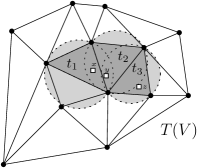
We will now prove an analog to Lemma 8 which shows that the triangles of do not contain many points of a new input on the average. Consider a triangle of and let be its circumscribed disk; is a Delaunay disk of . If a point lies in , we say that is in conflict with and call a conflict triangle for . Refer to Fig. 4. (The “conflict” terminology arises from the fact that if were added to , triangles with which it conflicts would no longer be in the Delaunay triangulation.) Let , the random variable that represents the points of that fall inside , the conflict set of . Furthermore, let . Note that the randomness comes from the random distribution of (on which and depend), as well as the randomness of . We are interested in the expectation over of . All expectations are taken over a random input chosen from .
Lemma 15.
For any triangle of , let be the conflict set of , and define . With probability at least over the construction of , we have and , for all triangles of .
Proof.
This is similar to the argument given in Lemma 8 with a geometric twist. Let the list of points be , the concatenation of through . Fix three distinct indices and the triangle with vertices (so we are effectively conditioning on ). Note that all the remaining points are chosen independently of , , from some distribution . For each , let be the indicator variable for the event that is inside . Let . Setting in (1), we get that if , then with probability at least . This is true for every fixing of , so it is also true unconditionally. By applying the same argument to any triple of distinct indices, and taking a union bound over all triples, we obtain that with probability at least , for any triangle generated by the points of , if , then . We henceforth assume that this event happens.
Consider a triangle of and its circumcircle . Since is Delaunay, contains no point of in its interior. Since is a -net for all disks with respect to , contains at most points of , that is, . This implies that , as in the previous paragraph. Since , we obtain , as claimed. Furthermore, since can be written as a sum of independent indicator random variables, Claim 9 shows that . ∎
4.1.2 Limiting Phase
We assume that we are done with the learning phase, and have with the property given in Lemma 15: for every triangle , and . We have reached the limiting phase where the algorithm is expected to compute the Delaunay triangulation with the optimal running time. We will prove the following lemma in this section.
Lemma 16.
Using the data structures from the learning phase, and the properties of them that hold with probability at least , in the limiting phase the Delaunay triangulation of input can be generated in expected time.
The algorithm, and the proof of this lemma, has two steps. In the first step, is used to quickly compute , with the time bounds of the lemma. In the second step, is computed from , using a randomized splitting algorithm proposed by Chazelle et al. [21], who provide the following theorem.
Theorem 17.
[21, Theorem 3] Given a set of points and its Delaunay triangulation, for any partition of into two disjoint subsets and , the Delaunay triangulations and can be computed in expected time, using a randomized algorithm.
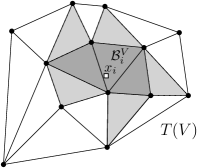
The remainder of this section is devoted to showing that can be computed in expected time . The algorithm is as follows. For each , we use to find the triangle of that contains it. By the properties of the ’s as described in §4.1.1, this takes expected time. We now need to argue that given the ’s, the Delaunay triangulation can be computed in expected linear time. For each , we walk through and find all the Delaunay disks of that contain , as in incremental constructions of Delaunay triangulations [12, Chapter 9]. This is done by breadth-first search of the dual graph of , starting from . Refer to Fig. 5. Let denote the set of triangles whose circumcircles contain . We remind the reader that is the conflict set of triangle .
Claim 18.
Given all ’s, all and sets can be found in expected linear time.
Proof.
To find all Delaunay disks containing , do a breadth-first search from . For any triangle encountered, check if contains . If it does not, then we do not look at the neighbors of . Otherwise, add to and to and continue. Since is connected in the dual graph of ,555Since the triangles in cover exactly the planar region of triangles incident to in . we will visit all ’s that contain . The time taken to find is . The total time taken to find all ’s (once all the ’s are found) is . Define the indicator function that takes value if and zero otherwise. We have
Therefore, by Lemma 15,
This implies that all ’s and ’s can be found in expected linear time. ∎
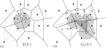
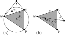
Our aim is to build the Delaunay triangulation in linear time using the conflict sets . To that end, we will use divide-and-conquer to compute the Voronoi diagram , using a scheme that has been used for nearest neighbor searching [24] and for randomized convex hull constructions [25, 20]. It is well known that the Voronoi diagram of a point set is dual to the Delaunay triangulation, and that we can go from one to the other in linear time [12, Chapter 9]. Refer to Fig. 6(a). Consider the Voronoi diagram of , . By duality, the vertices of correspond to the triangles in , and we identify the two. In particular, each vertex of has a conflict set , the conflict set for the corresponding triangle in , and , by our definition of (see Fig. 6(a)). We triangulate the Voronoi diagram as follows: for each region of , determine the lexicographically smallest Voronoi vertex in with minimum . Add edges from all the Voronoi vertices in to . Since each region of is convex, this yields a triangulation666We need to be a bit careful when handling unbounded Voronoi regions: we pretend that there is a Voronoi vertex at infinity which is the endpoint of all unbounded Voronoi edges, and when we triangulate the unbounded region, we also add edges to . By our bounding triangle assumption, there is no point in outside the convex hull of and hence the conflict set of is empty. of . We call it the geode triangulation of with respect to , [24, 20]. Refer to Fig. 6(b). Clearly, can be computed in linear time. We extend the notion of conflict set to the triangles in : Let be a triangle in and let , , be its incident Voronoi vertices. Then the conflict set of , , is defined as , where is the point whose Voronoi region contains the triangle . In the following, for any two points and , denotes the Euclidean distance between them.
Claim 19.
Let be a triangle of and let be its conflict set. Then the Voronoi diagram of restricted to , , is the same as the Voronoi diagram of restricted to , .
Proof.
Consider a point in the triangle , and let be the nearest neighbor of in . If , then has to be , since lies in the Voronoi region of with respect to . Now suppose that . Let be the perpendicular bisector of the line segment (ie, the line containing all points in the plane that have equal distance from and ). Refer to Figure 7. Let be the halfplane defined by that contains . Since intersects , by convexity it also contains a vertex of , say . Because and are on the same side (), . Note that has center and radius , because is a vertex of the Voronoi region corresponding to (in ). Hence, . It follows that , so , as claimed. ∎
Claim 19 implies that can be found as follows: for each triangle of , compute , the Voronoi diagram of restricted to . Then, traverse the edges of and fuse the bisectors of the adjacent diagrams, yielding .
Lemma 20.
Given , the Voronoi diagram can be computed in expected time.
Proof.
The time to find for a triangle in is [12, Chapter 7]. For a region of , let denote the set of triangles of contained in , and let denote the set of edges in incident to . Recall that denotes the common vertex of all triangles in . The total running time is , which is proportional to
since . For , let . Note that , by Lemma 15. We can write , where was the indicator random variable for the event that . Hence, since , Claim 9 implies that . Thus,
The number of edges in is linear, and each edge is incident to exactly two Voronoi regions . Therefore, . Furthermore, assembling the restricted diagrams takes time , and as , this is also linear. ∎
4.2 Running time analysis
In this section, we prove that the running time bound in Lemma 16 is indeed optimal. As discussed at the beginning of §4, Claim 5 implies that any comparison-based algorithm for computing the Delaunay triangulation of input needs at least expected comparisons. Recall that by Lemma 16, the expected running time of our algorithm is . The following is the main theorem of this section.
Theorem 21.
For , the entropy of the triangle of containing , and , the entropy of the Delaunay triangulation of , considered as a labeled graph,
Proof.
We first define some notation — for a point set and , let denote the neighbors of in . It remains to prove the following lemma.777A similar lemma is used in [22] in the context of hereditary algorithms for three-dimensional polytopes.
Lemma 22.
Given and , for every in we can compute the triangle in that contains in total expected time .
Proof.
First, we compute from and in linear time [19, 36]. Thus, we now know and , and we want to find for every point the triangle of that contains it. For the moment, let us be a little less ambitious and try to determine for each , a conflict triangle in , ie, is a triangle with . If and such that is an edge of , we can find a conflict triangle for in in time by inspecting all the incident triangles of in . Actually, we can find conflict triangles for all neighbors of in that lie in , by merging the two neighbor lists (see below). Noting that on average the size of these lists will be constant, we could almost determine all the , except for one problem: there might be inputs that are not adjacent to any in . Thus, we need to dynamically modify to ensure that there is always a neighbor present. Details follow.
Claim 23.
Let and write . Suppose that and are known. Then, in total time , for every , we can compute a conflict triangle of in .
Proof.
Let , and let be the triangle of incident to that is intersected by line segment . We claim that is a conflict triangle for . Indeed, since is an edge of , by the characterization of Delaunay edges (eg, [12, Theorem 9.6(ii)]), there exists an circle through and which does not contain any other points from . In particular, does not contain any other points from . Hence is also an edge of , again by the characterization of Delaunay edges applied in the other direction. Therefore, triangle is destroyed when is inserted into , and is a conflict triangle for in . It follows that the conflict triangles for can be computed by merging the cyclically ordered lists and . This requires a number of steps that is linear of the size of the two lists, as claimed. ∎
For certain pairs of points , the previous claim provides a conflict triangle . The next claim allows us to get from this, which is what we wanted in the first place.
Claim 24.
Let and let . Let be the conflict triangle for in incident to , as determined in Step 2c. Then we can find a conflict triangle for in in constant time.
Proof.
If , there is nothing to prove, so assume that . If has all vertices in , then it is also a triangle in , and we are trivially done. So assume that one vertex of is . Let be the edge of not incident to , and let be the endpoints of . We will show that is in conflict with at least one of the two triangles in that are incident to . Given , such a triangle can clearly be found in constant time. Refer to Fig. 8 for a depiction of the following arguments.
Since , by the characterization of Delaunay edges, it follows that is also an edge of . If does not lie in , then must also be in conflict with the other triangle that is incident to (since is intersected by the Delaunay edge ). Note that cannot have as a vertex and is a triangle of .
Suppose lies in . Since is a triangle in , the interior has no points other than . Thus, the segments and are edges of . These must also be edges of . But this means that must conflict with the triangle in incident to at the same side as . ∎
-
1.
Let be a queue containing the elements in .
-
2.
While .
-
(a)
Let be the next point in .
-
(b)
If , then insert into using the conflict triangle for , to obtain . If , then .
-
(c)
Using Claim 23, for each unvisited neighbor , compute a conflict triangle in .
-
(d)
For each unvisited neighbor , using , compute a conflict triangle of in . Then insert into , and mark it as visited.
-
(a)
The conflict triangles for all points in can now be computed using breadth-first search (see Algorithm 1). The loop in Step 2 maintains the invariant that for each point , a conflict triangle in is known. Step 2b is performed as in the traditional randomized incremental construction of Delaunay triangulations [12, Chapter 9]: walk from through the dual graph if to determine the conflict set of (as in the proof of Claim 18), insert new edges from all points incident to the triangles in to , and remove all the old edges that are intersected by these new edges. The properties of the conflict set ensure that this yields a valid Delaunay triangulation. By Claim 24, Step 2d can be performed in constant time.
The loop in Step 2 is executed at most once for each . It is also executed at least once for each point, since is connected and in Step 2d we perform a BFS. The insertion in Step 2b takes time. Furthermore, by Claim 23, the conflict triangles of ’s neighbors in can be computed in time. Finally, as we argued above, Step 2d can be carried out in total time. Now note that for , is proportional to , the number of triangles in in conflict with . Hence, the total expected running time is proportional to
Finally, using BFS as in the proof of Claim 18, given the conflict triangles , the triangles that contain the ’s can be found in expected time, and the result follows. ∎
4.3 The time-space tradeoff
We show how to remove the assumption that we have prior knowledge of the ’s (to build the search structures ) and prove the time-space tradeoff given in Theorem 3. These techniques are identical to those used in §3.2. For the sake of clarity, we give a detailed explanation for this setting. Let be any constant. The first rounds of the learning phase are used as in §4.1.1 to construct the Delaunay triangulation . We first build a standard search structure over the triangles of [12, Chapter 6]. Given a point , we can find the triangle of that contains in time.
The learning phase takes rounds, for some large enough constant . The main trick is to observe that (up to constant factors), the only probabilities that are relevant are those that are at least . In each round, for each , we record the triangle of that falls into. Fix , and for any triangle of , let be the number of times over the first rounds that . At the end of rounds, we take the set of triangles with . We remind the reader that is the probability that lies in triangle . The proof of the following lemma is identical to the proof of Lemma 10.
Lemma 25.
Fix . With probability at least , for every triangle of , if , then .
For every triangle in , we estimate as , and we use to build the approximate search structure . For this, we take the planar subdivision induced by the triangles in , compute the convex hull of , and triangulate the remaining polygonal facets. Then we use the construction of Arya et al. [10] to build an optimal planar point location structure for according to the distribution (the triangles of not in are assigned probability ). This structure has the property that a point in a triangle with probability can be located in steps [10, Theorems 1.1 and 1.2].
The limiting phase uses these structures to find for every : given , we use to search for it. If the search does not terminate in steps or fails to find (ie, ), then we use the standard search structure, , to find . Therefore, we are guaranteed to find in time. Clearly, each stores triangles, so by the bounds given in [10], each can be constructed with size in time. Hence, the total space is bounded by and the time required to build all the ’s is .
Now we just repeat the argument given in §3.2. Instead of doing it through words, we write down the expressions (for some variety). Let denote the time to search for given that . By Lemma 25, we have , so , for large enough, and thus . Thus,
We now bound the expected search time for .
Noting that for , we have , we get
If follows that the total expected search time is . By the analysis of §4.1 and Theorem 21, we have that the expected running time in the limiting phase is . If the conditions in Lemmas 15 and 25 do not hold, then the training phase fails. But this happens with probability at most . This completes the proof of Theorem 3.
5 Conclusions and future work
Our overall approach has been to deduce a “typical” instance for the distribution, and then use the solution for the typical instance to solve the current problem. This is a very appealing paradigm - even though the actual distribution could be extremely complicated, it suffices to learn just one instance. It is very surprising that such a single instance exists for product distributions. One possible way of dealing with more general distributions is to have a small set of typical instances. It seems plausible that even with two typical instances, we might be able to deal with some dependencies in the input.
We could imagine distributions that are very far from being generated by independent sources. Maybe we have a graph labeled with numbers, and the input is generated by a random walk. Here, there is a large dependency between various components of the input. This might require a completely different approach than the current one.
Currently, the problems we have focused upon already have time algorithms. So the best improvement in the running time we can hope for is a factor of . The entropy optimality of our algorithms is extremely pleasing, but our running times are always between and . It would be very interesting to get self-improving algorithms for problems where there is a much larger scope for improvement. Ideally, we want a problem where the optimal (or even best known) algorithms are far from linear. Geometric range searching seem to a good source of such problems. We are given some set of points and we want to build data structures that answer various geometric queries about these points [2]. Suppose the points came from some distribution. Can we speed up the construction of these structures?
A different approach to self-improving algorithms would be to change the input model. We currently have a memoryless model, where each input is independently drawn from a fixed distribution. We could have a Markov model, where the input depends (probabilistically) only on , or maybe on a small number of previous inputs.
References
- [1] Peyman Afshani, Jérémy Barbay, and Timothy M. Chan, Instance-optimal geometric algorithms, in Proc. 50th Annu. IEEE Sympos. Found. Comput. Sci. (FOCS), 2009, pp. 129–138.
- [2] Pankaj Agarwal and Jeff Erickson, Geometric range searching and its relatives, Advances in Discrete and Computational Geometry, (1998), pp. 1–56.
- [3] Alok Aggarwal, Leonidas J. Guibas, James Saxe, and Peter W. Shor, A linear-time algorithm for computing the Voronoi diagram of a convex polygon, Discrete Comput. Geom., 4 (1989), pp. 591–604.
- [4] Susanne Albers and Michael Mitzenmacher, Average case analyses of list update algorithms, with applications to data compression, Algorithmica, 21 (1998), pp. 312–329.
- [5] Susanne Albers and Jeffery Westbrook, Self-organizing data structures, in Online algorithms (Schloss Dagstuhl, 1996), vol. 1442 of Lecture Notes in Comput. Sci., Springer Verlag, Berlin, 1998, pp. 13–51.
- [6] Brian Allen and Ian Munro, Self-organizing binary search trees, J. ACM, 25 (1978).
- [7] Noga Alon and Joel H. Spencer, The probabilistic method, Wiley-Interscience Series in Discrete Mathematics and Optimization, Wiley-Interscience, New York, second ed., 2000.
- [8] Sigal Ar, Bernard Chazelle, and Ayellet Tal, Self-customized BSP trees for collision detection, Comput. Geom. Theory Appl., 15 (2000), pp. 91–102.
- [9] Sanjeev Arora and Boaz Barak, Computational Complexity: A Modern Approach, Cambridge University Press, 2009.
- [10] Sunil Arya, Theocharis Malamatos, David M. Mount, and Ka Chun Wong, Optimal expected-case planar point location, SIAM J. Comput., 37 (2007), pp. 584–610.
- [11] Jon L. Bentley and Catherine C. McGeoch, Amortized analyses of self-organizing sequential search heuristics, Comm. ACM, 28 (1985), pp. 404–411.
- [12] Mark de Berg, Otfried Cheong, Marc van Kreveld, and Mark Overmars, Computational Geometry: Algorithms and Applications, Springer-Verlag, Berlin, third ed., 2008.
- [13] James R. Bitner, Heuristics that dynamically organize data structures, SIAM J. Comput., 8 (1979), pp. 82–110.
- [14] Jean-Daniel Boissonnat and Mariette Yvinec, Algorithmic geometry, Cambridge University Press, 1998.
- [15] Allan Borodin and Ran El-Yaniv, Online computation and competitive analysis, Cambridge University Press, 1998.
- [16] Kevin Buchin and Wolfgang Mulzer, Delaunay triangulations in time and more, in Proc. 50th Annu. IEEE Sympos. Found. Comput. Sci. (FOCS), 2009, pp. 139–148.
- [17] Timothy M. Chan and Mihai Pǎtraşcu, Voronoi diagrams in time, in Proc. 39th Annu. ACM Sympos. Theory Comput. (STOC), 2007, pp. 31–39.
- [18] , Transdichotomous results in computational geometry, I: Point location in sublogarithmic time, SIAM J. Comput., 39 (2009), pp. 703–729.
- [19] Bernard Chazelle, An optimal algorithm for intersecting three-dimensional convex polyhedra, SIAM J. Comput., 21 (1992), pp. 671–696.
- [20] , The discrepancy method, Cambridge University Press, 2000.
- [21] Bernard Chazelle, Olivier Devillers, Ferran Hurtado, Mercè Mora, Vera Sacristán, and Monique Teillaud, Splitting a Delaunay triangulation in linear time, Algorithmica, 34 (2002), pp. 39–46.
- [22] Bernard Chazelle and Wolfgang Mulzer, Computing hereditary convex structures, in Proc. 25th Annu. ACM Sympos. Comput. Geom. (SoCG), 2009, pp. 61–70.
- [23] , Markov incremental constructions, Discrete Comput. Geom., 42 (2009), pp. 399–420.
- [24] Kenneth L. Clarkson, A randomized algorithm for closest-point queries, SIAM J. Comput., 17 (1988), pp. 830–847.
- [25] Kenneth L. Clarkson and Peter W. Shor, Applications of random sampling in computational geometry, II, Discrete Comput. Geom., 4 (1989), pp. 387–421.
- [26] Kenneth L. Clarkson and Kasturi Varadarajan, Improved approximation algorithms for geometric set cover, Discrete Comput. Geom., 37 (2007), pp. 43–58.
- [27] Thomas H. Cormen, Charles E. Leiserson, Ronald L. Rivest, and Clifford Stein, Introduction to Algorithms, MIT Press, third ed., 2009.
- [28] Thomas M. Cover and Joy A. Thomas, Elements of information theory, Wiley-Interscience, second ed., 2006.
- [29] Herbert Edelsbrunner and Ernst P. Mücke, Simulation of simplicity: a technique to cope with degenerate cases in geometric algorithms, ACM Trans. Graph., 9 (1990), pp. 66–104.
- [30] Vladmir Estivill-Castro and Derick Wood, A survey of adaptive sorting algorithms, ACM Comput. Surv., 24 (1992), pp. 441–476.
- [31] Michael L. Fredman, How good is the information theory bound in sorting?, Theoret. Comput. Sci., 1 (1975/76), pp. 355–361.
- [32] Gaston H. Gonnet, J. Ian Munro, and Hendra Suwanda, Exegesis of self-organizing linear search, SIAM J. Comput., 10 (1981), pp. 613–637.
- [33] Yijie Han, Deterministic sorting in time and linear space, J. Algorithms, 50 (2004), pp. 96–105.
- [34] Yijie Han and Mikkel Thorup, Integer sorting in expected time and linear space, in Proc. 43rd Annu. IEEE Sympos. Found. Comput. Sci. (FOCS), 2002, pp. 135–144.
- [35] James H. Hester and Daniel S. Hirschberg, Self-organizing linear search, ACM Comput. Surv., 17 (1985), pp. 295–311.
- [36] David G. Kirkpatrick, Efficient computation of continuous skeletons, in Proc. 20th Annu. IEEE Sympos. Found. Comput. Sci. (FOCS), 1979, pp. 18–27.
- [37] Der Tsai Lee, On -nearest neighbor Voronoi diagrams in the plane, IEEE Trans. Comput., 31 (1982), pp. 478–487.
- [38] Jiří Matoušek, Reporting points in halfspaces, Comput. Geom. Theory Appl., 2 (1992), pp. 169–186.
- [39] Jiří Matoušek, Raimund Seidel, and E. Welzl, How to net a lot with little: small -nets for disks and halfspaces, in Proc. 6th Annu. ACM Sympos. Comput. Geom. (SoCG), 1990, pp. 16–22.
- [40] John McCabe, On serial files with relocatable records, Operations Res., 13 (1965), pp. 609–618.
- [41] Kurt Mehlhorn, Data structures and algorithms 1: Sorting and Searching, EATCS Monographs on Theoretical Computer Science, Springer Verlag, Berlin, 1984.
- [42] Rajeev Motwani and Prabhakar Raghavan, Randomized algorithms, Cambridge University Press, 1995.
- [43] Evangelia Pyrga and Saurabh Ray, New existence proofs for -nets, in Proc. 24th Annu. ACM Sympos. Comput. Geom. (SoCG), 2008, pp. 199–207.
- [44] Ronald Rivest, On self-organizing sequential search heuristics, Comm. ACM, 19 (1976), pp. 63–67.
- [45] Daniel D. Sleator and Robert E. Tarjan, Amortized efficiency of list update and paging rules, Comm. ACM, 28 (1985), pp. 202–208.
- [46] , Self-adjusting binary search trees, J. ACM, 32 (1985), pp. 652–686.
Appendix A Constructing the -net
Recall that . Given a set of points in the plane, we would like to construct a set of size such that any open disk with intersects . (This is a -net for disks.) We describe how to construct in deterministic time , using a technique by Pyrga and Ray [43]. This is by no means the only way to obtain . Indeed, it is possible to use the older techniques of Clarkson and Varadarajan [26] to get a another—randomized—construction with a better running time.
We set some notation. For a set of points , a -set of is a subset of of size obtained by intersecting with an open disk. A -set is is such a subset with size more than . We give a small sketch of the construction. We take the collection of all -sets of . We need to obtain a small hitting set for . To do this, we trim to a collection of -sets that have small pairwise intersection. Within each such set, we will choose an -net (for some ). The union of these -nets will be our final -net. We now give the algorithmic construction of this set and argue that it is a -net. Then, we will show that it has size .
It is well known that the collection has sets [25, 37] and that an explicit description of can be found in time [3, 37], since corresponds to the -th-order Voronoi diagram of , each of whose cells represents some -set of [37]. Let be a maximal subset of such that for any , . We will show in Claim 26 how to construct in time. To construct , take a -net for each , and set .888That is, is a subset of such that any open disk that contains more than points from intersects . It is well known that each has constant size and can be found in time [20, p. 180, Proof I]. The set is an -net for : if an open disk intersects in more than -points, by the maximality of , it must intersect a set in more than points. Now contains a -net for (recall that ), so must meet the disk . We will argue in Claim 27 that . This completes the proof.
Claim 26.
The set can be constructed in time .
Proof.
We use a simple greedy algorithm. For each , construct the collection of all -sets of . The set has size , and the total number of disks defined by the points in is at most . Thus, there are at most sets in , and they can all be found in time. Since there are at most sets (as we argued earlier), the total number of -sets is , and they can be obtained in time. Next, perform a radix sort on the multiset . This again takes time . Note that for any , precisely if and share some -set. Now is obtained as follows: pick a set , put into , and use the sorted multiset to find all that share a -set with . Discard those from . Iterate until is empty. The resulting set has the desired properties. ∎
Claim 27.
.
Proof.
The set is the union of -nets for each set . Since each net has constant size, it suffices to prove that has sets. This follows from a charging argument due to Pyrga and Ray [43, Theorem 12]. They show [43, Lemma 7] how to construct a graph on vertex set with at most edges with the following property: for , let be the set of all that contain , and let be the induced subgraph on vertex set . Then, for all , . Thus,
Consider the sum . All sets in contain exactly points, so each set contributes to the sum. By double counting, . Furthermore, an edge can appear in only if , so again by double-counting,
Hence, , and . ∎