Scaling Relations for Contour Lines of Rough Surfaces

Abstract

Equilibrium and non-equilibrium growth phenomena, e.g., surface growth, generically yields self-affine distributions. Analysis of statistical properties of these distributions appears essential in understanding statistical mechanics of underlying phenomena. Here, we analyze scaling properties of the cumulative distribution of iso-height loops (i.e., contour lines) of rough self-affine surfaces in terms of loop area and system size. Inspired by the Coulomb gas methods, we find the generating function of the area of the loops. Interestingly, we find that, after sorting loops with respect to their perimeters, Zipf-like scaling relations hold for ranked loops. Numerical simulations are also provided in order to demonstrate the proposed scaling relations.

Keywords: Rough Surface, Contour Line, Self Affine, Zipf’s Law.
PACS number(s): 47.27.eb,

1 Introduction

Self-affine distributions are ubiquitous in many phenomena in nature, such as in growing surfaces and interfaces [1, 2, 3, 4], fractured media [5, 6], and graphs of two-dimensional turbulent flows [4, 7]. Self-affine distributions have also been used as a tool to study scaling properties of two-dimensional statistical models by mapping these models to a two-dimensional Coulomb gas [8, 9]. Moreover, crystal growth, the growth of bacterial colonies, and the formation of clouds in the upper atmosphere [10] are all examples of non-equilibrium phenomena which grow self-affine rough surfaces. The above applications on a fundamental level make the surface-growth problem as a paradigm for a broad class of problems in the context of non-equilibrium statistical mechanics.

Self-affine surfaces can be described by their height distribution function. From statistical point of view, it is necessary to explore topography of this kind of surfaces. In such surfaces, heights are invariant under re-scaling, namely $h(\textbf{r})\cong b^{-H}h(b\textbf{r})$, where $H$ is called the roughness exponent or the Hurst exponent. It implies that in a self-affine surface, the variance of the surface height, i.e., $\sqrt{\langle[h(\textbf{x})-\langle{h}\rangle]^{2}\rangle}$, scales as $L^{H}$, where $L$ is the size of the system and average is taken over $x$. If we require translational and rotational invariance of the surface then the structure function of this surface behaves as

$$C_{2}(\textbf{r})=\langle[h(\textbf{x})-h(\textbf{x}+\textbf{r})]^{2}\rangle\sim|\textbf{r}|^{2H}.$$ (1.1)

The above equation gives a simple formula to calculate the roughness exponent. To determine that a given surface is self-affine or multi-affine we need to measure the $p$th order structure function defined by $C_{p}(\textbf{r})=\langle|h(\textbf{x})-h(\textbf{x}+\textbf{r})|^{p}\rangle$. The exponent hierarchy $\alpha_{p}$ is defined through the relation $C_{p}(r)\simeq r^{\alpha_{p}H}$. The exponent $\alpha_{p}$ varies linearly with $p$ for a self-affine surface. For a multi-affine surface, instead, it would vary non-linearly with $p$ [11]. The Fourier space counterpart of the structure function is Fourier power spectrum $S(\textbf{q})=\langle|h(\textbf{q})|^{2}\rangle$, where $h(\textbf{q})$ is the Fourier transform of $h(\textbf{r})$. Equation (1.1) gives the scaling relation for the power spectrum, i.e., $S(\textbf{q})\sim|\textbf{q}|^{-2(1+H)}$, for small values of $q$ or large values of $r$. One way to generate a Gaussian ensemble of self-affine surfaces is by taking each Fourier height as an independent Gaussian random variable with variance given by $S(\textbf{q})\sim|\textbf{q}|^{-2(1+H)}$. In other words,

$$P\{h\}\sim\exp\left[-\frac{k}{2}\int_{0}^{\Lambda}d^{2}\textbf{q}\ \textbf{q}^{2(1+H)}h_{\textbf{q}}h_{-\textbf{q}}\right],$$ (1.2)

where $\Lambda=1/a$ is the high-momentum cutoff and $k$ is the stiffness. A family of self-affine surfaces having all the required properties can be generated by the above distribution. For rough surfaces with unbounded heights we have $0\leq H<1$, where the higher $H$ is related to smoother surface with hills. In a self-affine distribution $H>1/2$ ($H<1/2$), it implies positive (negative) correlations among the increments of the generated values, $H=1/2$ means that the statistics of the surface follows that of a Brownian motion. At $H=0$, it is possible to write Eq. (1.2) in the real space by using ordinary derivative $P\{h\}\sim\exp\left[-\frac{k}{2}\int_{0}^{L}d^{2}\textbf{x}(\partial_{\textbf{x}}h)^{2}\right]$. For the general case we should replace ordinary derivative with the fractional one, that is, $P\{h\}\sim\exp\left[-\frac{k}{2}\int_{0}^{L}d^{2}\textbf{x}h(-\nabla^{2})^{1+H}h\right]$, where the fractional derivative is defined by $(-\nabla^{2})^{1+H}e^{i{\bf q}.{\bf x}}=-|q|^{2+2H}e^{i{\bf q}.{\bf x}}$ (for more details see [12]).

The contour lines that are generated by a cut through the surface at a certain height are important in characterizing self-affine surfaces.

In Fig. $1$ we plotted an example of the set of contour lines of a rough surface. The statistical properties of contour lines of rough surfaces show fractal behavior. The accepted fractal dimension of a contour line $D=\frac{3-H}{2}$ was found by Kondev and Henley (KH) by using scaling arguments [13]. Recently, Schramm and Sheffield [14] proved rigorously that the contour lines of Gaussian free field with $H=0$ are conformally invariant with fractal dimension $D=\frac{3}{2}$, which is in agreement with the KH result. Conformally invariant curves in statistical physics can be investigated by Coulomb gas field theory [8]. The most well-known loop model that can be investigated by this field theory is the $O(n)$ model, which can be defined on the honeycomb lattice as follows: take the ensemble of loops on the honeycomb lattice so that the generating function of the model is given by $Z=\sum x^{l}n^{N}$, where $N$ and $l$ are number of the loops and bonds, respectively, $n$ is the weight of each loop, and $x$ is the weight of each bond. At the critical point, this loop model can be investigated, after mapping the loop model to the solid on solid (SOS) model [8], by the free field theory $P\{h\}\sim\exp[-\frac{k}{2}\int_{0}^{L}d^{2}x(\partial h)^{2}]$. It is also possible to find the scaling exponents of conformal curves by the above field theory [8].

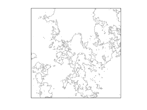
Figure 1: Small part of contour lines of a rough surface with size $3000^{2}$ and $H=0.5$; by zooming in on the picture one can see many small loops.

Since the height ensemble of a rough surface is not conformally invariant, rigorous investigating of their contour lines is more difficult than the Coulomb gas case. Indeed, one can not employ the powerful tools of conformal field theory (CFT) to study this system. For a rough surface with a generic $H$ there is no rigorous proof for results obtained by KH [15]. Nonetheless, it seems that the contour line ensemble shows scaling properties similar to the conformal curves encountered in some models such as the contour lines of tungsten oxide ($WO_{3}$) [16] and KPZ surfaces [17].

In this paper, by using techniques which are common in the realm of Coulomb gas field theory, we introduce new scaling laws for some properties of contour lines of self-affine rough surfaces. The scaling properties of the cumulative distribution of the number of contours versus the area of the contours and the size of the system are also obtained. In addition, we find a close relation between the cumulants of $A$, the area of contour lines, and the eigenvalues of the fractional Laplacian. Finally, we introduce the scaling property of ranked contour lines versus both rank and system size (Zipf’s law). Numerical simulations are also provided to substantiate our analysis.

2 Numerical methods

To generate self-affine rough surfaces in our numerical simulations,

we have used the successive random addition method [18]. In our simulations we have generated surfaces of size $L\times L$ with $L\in\{400,600,800,1200,2000,3000,4000\}$. To investigate the effect of roughness exponent on the scaling relations we used several values of $H\in\{0.3,0.4,0.5,0.6,0.7\}$. In each case, all calculations have been averaged over 200 realizations.

To generate the loops in the contour lines we used a contouring algorithm that treats the input matrix as a regularly spaced grid. The algorithm scans this matrix and compares the values of each block of four neighboring elements (i.e., a plaquette) in the matrix to the contour level values. If a contour level falls within a cell, the algorithm performs a linear interpolation to locate the point at which the contour crosses the edges of the cell. The algorithm connects these points to produce a segment of a contour line. After generating the contours of a given surface, in order to eliminate the effect of the edges of the lattice we have excluded the contours crossing the edges of the lattice.

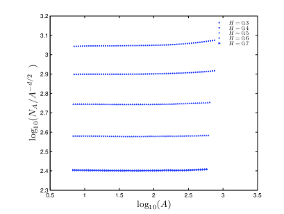
Figure 2: Scaling relation for cumulative distribution of areas. Curves show $\frac{N_{A}}{A^{-d/2}}$ for rough surfaces with size $4000^{2}$ and different roughness exponents.

To show the goodness of the fits and consistency of our simulations with theory, we used the following three different methods for estimating the exponents: (a) we numerically calculated local slops of the curves by fourth-order numerical differentiation for non-uniform data points; e.g., in the case of Eq. (3.2), derivation of $\log_{10}(N_{A})$ relative to $\log_{10}A$. (b) We present some of the curves by dividing both sides of a scaling relation to the claimed power law to show how seriously they are aligned or how they deviate from a horizontal line, e.g., Fig. 2. And, (c) We used Bayesian analysis without prior distribution, namely Likelihood analysis [19, 20, 21, 22] to calculate the accuracy of the exponent generated from our numerical results.

3 Cumulative distribution of area

A key difference between the contour lines in Coulomb gas field theory and the self-affine rough surfaces is in the fractal dimension of the set of all contour lines. For a given self-affine rough surface, this fractal dimension is $d=2-H$. It is well-known that many of the scaling relations in Coulomb gas field theory remain unchanged just by substituting this $d$ as the dimension of our set. To give an example, let us define the fractal dimension of a contour line $D$ as $\textit{l}\sim\textit{R}^{D}$, where l is the the perimeter of the contour and R is the radius of gyration. Moreover, the probability of finding a contour loop with length l is $N_{\textit{l}}\sim\textit{l}^{-\tau}$. One can show that there is a hyperscaling relation between the scaling exponents $D$ and $\tau$ as follows:

$$D(\tau-1)=d,$$ (3.1)

which is exactly the same as the hyperscaling relation for domain walls in statistical models [23]. Following KH, the cumulative distribution of the number of contours with area greater than $A$ has the following form:

$$N_{A}\sim\frac{C}{A^{{d}/{2}}}.$$ (3.2)

This gives the right answer for Coulomb gas loops with zero roughness exponent [23]. In the rest of the paper using new conjectures we will demonstrate some other evidences to support the above relation. This in turn leads us to several new scaling relations.

We checked Eq. (3.2) by using numerical simulations for different $H$’s, see Fig $2$. As is shown, we plot $\log_{10}(\frac{N_{A}}{A^{-d/2}})$ versus $\log_{10}(A)$ to show how seriously they follow Eq. (3.2). The straight horizontal curves exhibit that the proposed scaling relation is preserved up to $2$ orders of magnitude of $A$. As is seen, in the case of $H=0.3$ we have a small deviation from the proposed exponent at large values of $A$, which is related to finite-size effects. For a given lattice size and for small values of $H$, there are not so many large contour lines, but we have many small ones. This is led by the nature of self-affinity at small Hurst exponents. There are no deviations when we increase $H$ (Fig. 2). In Table 1, we report the best fit values calculated by the likelihood analysis [19, 20, 21, 22] at $68.3\%$ and $95.4\%$ confidence levels.

$H$	Theory	Local exponent ($1\sigma$)	Local exponent ($2\sigma$)
$0.3$	-0.850	$-0.840\pm{0.010}$	$-0.840\pm{0.020}$
$0.4$	-0.80	$-0.795\pm{0.006}$	$-0.795\pm{0.020}$
$0.5$	-0.750	$-0.752\pm{0.010}$	$-0.752\pm{0.025}$
$0.6$	-0.700	$-0.703\pm{0.005}$	$-0.703\pm{0.020}$
$0.7$	-0.650	$-0.652\pm{0.005}$	$-0.652\pm{0.020}$

Table 1: The best fit values of exponent $d/2$ derived by using the likelihood method. $\sigma$ denotes standard deviation of each calculated exponent.

For loops corresponding to surfaces with $H=0$, using Coulomb gas techniques, Cardy and Ziff showed that $C$ has the universal form as a function of the system size $L$ for different critical statistical physics models [24]. To calculate $C$, Cardy and Ziff evaluated the total area inside all loops using two different methods, and then they found the universal form of $C$. Inspired by this method, we argue to give some new scaling relations for contour lines of self-affine rough surfaces. Using Eq. (3.2) it is straightforward to show that $\langle A_{tot}\rangle=CL^{H}$, for $0<H<1$, and for $H=0$ it has a logarithmic form.

Let us consider a typical point $x$ with height $h$ above the horizon (we cut our self-affine surface by a plane). If we draw a circle of radius $h^{{1}/{H}}$ around the point, since we are dealing with a rough surface, all points inside the circle will be above the horizon. In other words, inside the loop is a compact region with the fractal dimension 2. Since the fractal dimension of the clusters is 2, one could obtain the total area of the clusters proportional to the area of the system. This is just a lower bound for the interior areas of the loops — see [25]. In addition, it is also possible to see from simulation that by cutting the surface from the average height one could get always clusters of the order of the system size. Thus one can get the following scaling relation for $C$ with respect to the system size:

$$C\sim L^{2-H}.$$ (3.3)

This indicates that the number of contour lines with area greater than $A$ per total length of all contours, i.e., $L^{2-H}$, is independent of the system size. It is also worth noting that the cumulative distribution of the contours with area $A$ is independent of $a$, the ultraviolet cutoff, which is another length scale. Our simulations confirm the validity of the scaling relation (3.3) for different values of $H$, see Fig. $3$.

The above result is also useful to get another nontrivial equation for contour lines. To calculate the total area we can use the formula

$$\langle A_{tot}\rangle=\int<d(r)>\textit{d}^{2}\textit{r},$$ (3.4)

in which $d(r)$ is the minimum number of loops which must be crossed to connect $r$ to the edge of the lattice. Since the total area inside the loops is proportional to the area of the system, we conclude

$$d(r)\sim(\frac{r}{L})^{2H}.$$ (3.5)

This is reminiscent of the height correlation function in the self-affine rough surfaces. For $H=0$ the relation is logarithmic and was proved explicitly in [24].

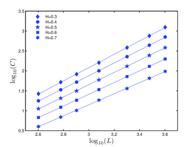
Figure 3: Scaling relation for the coefficient of cumulative distribution of areas for rough surfaces with respect to system size for different values of $H$ as shown in the graph. Slops of the curves from top to bottom are given by $1.66\pm 0.04$, $1.60\pm 0.03$, $1.53\pm 0.03$, $1.46\pm 0.04$, and $1.37\pm 0.04$.

These results show that one may investigate contour loops of rough surfaces by defining currents for the loops. Again, by analogy with the Coulomb gas methods one can define $\textit{J}_{\mu}(x,y)\sim\sqrt{g}\frac{\epsilon_{\mu\nu}\partial_{\nu}h}{L^{H}}$ as the current density of loops. This is a natural candidate if we imagine that the height function is extended to the two-dimensional manifold in such a way that it is constant within each plaquette. Normalization with respect to width is necessary because we have a rough surface where width is changing by size. This definition for the current density means that we can map our height model to the contour lines or vice versa. Since iso-height lines have the same role as the domain walls between the positive and negative heights, the directional derivative of $h$ along a contour must be zero and it must vary along a line normal to the contour. Using the above function to parameterize the geometry of contour line, it is possible to write

$$A=-\frac{1}{2}\int\int|x-x^{\prime}|\delta(y-y^{\prime})J_{y}(x,y)J_{y}(x^{\prime},y^{\prime})d\textbf{r}d\textbf{r}^{\prime}.$$ (3.6)

This equation is independent of our definition of currents. By using simple dimensional analysis, it is not difficult to find our special normalization, i.e., $\frac{1}{L^{H}}$. One can check that Eq. (3.6) gives $<A_{tot}>\sim L^{2}$. Using Eq. (3.6), inspired by Cardy’s argument [23], we find the generating function of the cumulants of area of contour loops. The argument for getting cumulants of area is as follows. For the simplicity, we use the Dirichlet boundary condition, $h=$const, on the boundary of the system, which means that loops do not cross the boundary. After integration by parts, Eq. (3.6) gives $A\simeq\int d^{2}rh^{2}(r)$. In simulation and experiment there are many curves emerging from the boundary and going back to another point in the boundary; therefore, there will be no exact Dirichlet boundary condition.

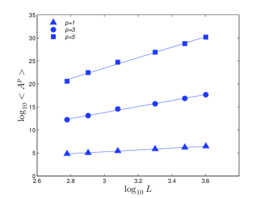
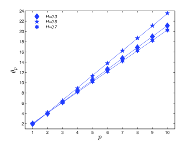
Figure 4: Top: Moments $\left\langle A^{p}\right\rangle$ of loop areas of rough surfaces versus system size; for $p=1,3$, and $5$. Here we have the exponents $\theta_{1}=2.02\pm 0.06$, $\theta_{3}=6.05\pm 0.55$, and $\theta_{5}=11.03\pm 1.06$.   Bottom: $\theta_{p}$ versus $p$ for surfaces with size $4000^{2}$ with different roughness exponents $H$ as indicated on the graph.

However, as we will see in the simulations, many of our scaling relations, especially the distribution of contours, are independent of the boundary conditions. By using the real space representation of the height distribution and the Gaussian integral, one can derive

$$\langle e^{-uA}\rangle=\frac{\det(-\partial^{2+2H}+\frac{2gu}{kL^{2H}})^{-1/2}}{\det(-\partial^{2+2H})^{-1/2}}.$$ (3.7)

where $k$ is the stiffness and $u$ is an auxiliary field. One can write the above equation as an infinite sum by using Fourier transform

$$\langle e^{-uA}\rangle=e^{-\frac{1}{2}\sum_{m}\ln\left(1+\frac{2guL^{2}}{k\lambda_{m}}\right)},$$ (3.8)

where $\frac{\lambda_{m}}{L^{2+2H}}$ are the eigenvalues of the fractional Laplacian with Dirichlet boundary conditions [12]. Expanding Eq. (3.8) gives the higher cumulants of $A$,

$$\langle A^{p}\rangle\sim L^{2p}\sum_{m}\frac{1}{\lambda_{m}^{p}}.$$ (3.9)

The sum is convergent for all values of $p$ and $H$ except $p-1=H=0$, which is logarithmic with respect to $L$. To check the above equation we calculated $\langle A^{p}\rangle$ for surfaces with different roughness exponents and different sizes. For $p=1$ all of the surfaces have $\langle A^{1}\rangle\sim L^{\theta}$ with $\theta=2\pm 0.05$. For higher moments one can write $\langle A^{p}\rangle\sim L^{\theta_{p}}$ with $\theta_{p}\sim\theta_{1}p$. For surfaces with roughness exponent between $0.3$ and $0.7$, the exponent $\theta_{1}$ varies from $1.94$ to $2.15$ . One can see in Fig. 4b that all of the $\theta_{p}$’s are linear with respect to $p$. The deviation from $\theta=2$ could be related to our restriction in getting larger sizes in simulation.

4 Zipf’s law for contour lines

Another interesting scaling relation is the universality of the distribution of the ranked loop perimeters, which is named Zipf’s law [26]. Following [26, 27], the average perimeter of the nth largest cluster can be found by Eq. (3.2), which is called by Mandelbrot the Zipf distribution

$$\textit{l}_{\textit{n}}\sim\frac{L^{D}}{n^{\frac{D}{d}}},$$ (4.1)

where $d$ is the fractal dimension of all loops and $D$ is the fractal dimension of one of loops. We should emphasize that we have normalized the equation with the appropriate power of total number of contour loops, so we ignore here the scaling of the total number of loops [26]. We have numerically checked this scaling relation for self-affine surfaces, both with respect to rank $n$ and the system size $L$. As shown in Fig. $5$, in three subfigures (for $H\in\{0.3,0.5,0.7\}$) for eight different realizations, we presented the log-log plot of $\frac{l_{n}}{n^{-D/d}}$ versus $n$. Here, ${l_{n}}$ shows a scaling relation according to Eq. (4.1). For the case of $H=0.3$, the scaling relation is preserved for over 2 orders of magnitude of $n$. Since the number of small loops is few, in larger values of $H=0.5,0.7$, we could see the agreement just for 1 order of magnitude.

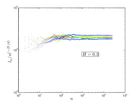
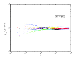
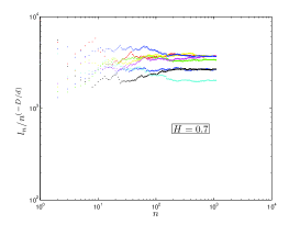
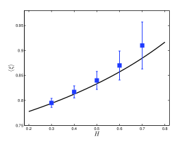
Figure 5: Top left ($H=0.3$), right($H=0.5$), and bottom left ($H=0.3$): for system size of $L=4000$, the curves of ranked loop perimeters divided by $n^{-D/d}$ vs rank numbers are shown for eight different realizations. Bottom right: the squares stand for the averaged $\xi$ (the numerical estimated exponent) over $200$ realizations. The solid line shows the theoretical relation between $\xi$ and $H$, i.e., $\xi=\frac{D}{d}$.

To calculate the exponent in our numerical results let us consider $l_{n}\sim n^{-\xi}$. We calculated the exponent; Fig.  $5$ (bottom right) depicts the variation of $\xi$ versus $H$ (the average is over different realizations). Since in higher $H$s we have lower number of loops, thus $\xi$ of higher values of $H$ have lower accuracy. We also numerically checked the relation of $\textit{l}_{\textit{n}}$ versus $L$. In the case of $H=0.3$, we obtained a scaling relation with exponent $1.38\pm 0.03$, which is near theoretical value $1.35$. In higher values of $H$, the estimated exponents are not sufficiently accurate because the number of loops in smaller system sizes is low. With the same method one can find the average area and the radius of gyration as a function of rank

$$A_{\textit{n}}\sim\frac{L^{2}}{n^{\frac{2}{d}}},\hskip 56.9055ptR_{\textit{n}}\sim\frac{L}{n^{\frac{1}{d}}}.$$ (4.2)

Both of the above formulas are in good agreement with our numerical results. In these kinds of scaling relations the error of the estimated exponents for large system sizes are considerably small. We believe Eqs (4.1) and (4.2) provide a good method to calculate the fractal dimension of a single contour as well as the fractal dimension of all contours.

5 Discussion and Conclusion

In summary, by using field theory of rough surfaces and considering current for the model, we confirmed the previously known scaling relation for cumulative distribution of area. In addition, we found a new scaling relation for this distribution with respect to system size. Since the action is not translationally invariant and the small momenta are important, naturally scaling properties depend to the system size. It seems that large momenta do not contribute in the scaling properties. Although system is not invariant under homogeneous translation, it is not difficult to see that it is invariant under $h\rightarrow h+\epsilon_{\mu\nu}a^{\mu}x^{\nu}$, which means it is inhomogeneously translational invariant. Using inhomogeneous translation one can define the currents $\textit{J}_{\mu}(x,y)\sim\epsilon_{\mu\nu}\partial^{1-H}_{\nu}h$ corresponding to Wilson loops of the theory and re-derive the results of Sec.  II. Since we only investigated the scaling properties of the contour lines, these two different given currents lead to the same scaling relations.

Considering these currents for contour lines we think that there may be a close relation between the statistics of these lines and the eigenvalues of fractional Laplacian. In this paper, we discussed leading scaling behavior with respect to the system size, however, to see the effect of the eigenvalues of the fractional Laplacian one needs more careful study of the amplitudes as well. Since there is no conformal invariance in the height ensemble, finding the exact values of $d(r)$ and $C$ using the techniques of the Coulomb gas is not tractable.

We confirmed our proposed scaling relations by simulations through cutting a self-affine surface at different heights. We have only interpreted the results for the case of cutting the surface at its mean height. But we checked also all of the scaling relations for the cases of cutting the surface at heights $h=\{0.1,0.2,0.3,0.4,0.5,0.6,0.7,0.8,0.9\}\sigma$, where $\sigma$ is the height variance of the surface. We have not seen any meaningful deviation from what we obtained for the mean height.

We also introduced new Zipf-like scaling relations for the contour lines of self-affine rough surfaces, and verified them via simulations. We believe the same scaling relations are applied to the clusters of rough surfaces but with different exponents.

ACKNOWLEDGMENTS

The work of S.M.V.A. was supported in part by the Research Council of the University of Tehran. We thank A. Rezakhani Tayefeh, M. Habibi, H. Mohseni Sadjadi, A. Naji, M. Nouri-Zonoz, and M. Yaghoubi for useful discussions. We are grateful of N. Abedpour, M. F. Miri, and M. Sadegh Movahed for useful comments. We are also indebted anonymous referees for their enlightening comments.

References

- [1] A. -L. Barabasi and H. E. Stanley, Fractal Concepts in Surface Growth (Cambridge University Press, New York, 1995).
- [2] J. Kondev, C. L. Henley, and D. G. Salinas, Phys. Rev. E 61, 164 (2000).
- [3] A. I. Zad, G. Kavei, M. R. R. Tabar, and S. M. V. Allaei, J. Phys: Condens. Matter 15, 1889 (2003).
- [4] M. B. Isichenko, Rev. Mod. Phys. 64, 961 (1992).
- [5] M. Sahimi, Phys. Rep. 306, 213 (1998).
- [6] G. Drazer, H. Auradou, J. Koplik, and J. P. Hulin, Phys. Rev. Lett. 92, 014501 (2004).
- [7] R. Ramshankar and J. P. Gollub, Phys. Fluids A 3, 1344 (1991).
- [8] B. Nienhuis, in Phase Transition and Critical Phenomena, edited by C. Domb and J. L. Lebowitz (Academic, London, 1987) , Vol. 11.
- [9] J. L. Jacobsen and J. Kondev, Nucl. Phys. B 532, 635 (1998).
- [10] J. D. Pelletier, Phys. Rev. Lett. 78, 2672 (1997).
- [11] A. L. Barabasi, R. Bourbonnais, M. Jensen, J. Kertesz, T. Vicsek, and Y. C. Zhang, Phys. Rev. A 45, R6951 (1992).
- [12] H. M. Srivastava, and J. J. Trujiilo, Theory and Applications of Fractional Differential Equations, (Elsevier, Amsterdam, 2006).
- [13] J. Kondev and C. L. Henley, Phys. Rev. Lett. 74, 4580 (1995).
- [14] O. Schramm and S. Sheffield, Acta Mathematica, 202, 21 (2009), e-print arXiv:math.PR/0605337.
- [15] M. Schwartz redrived the KH result for the special cases by Flory’s argument: M. Schwartz, Phys. Rev. Lett. 86, 1283 (2001).
- [16] A. Saberi, M. A. Rajabpour, and S. Rouhani, Phys. Rev. Lett. 100, 044504 (2008); eprint arXiv:07122984.
- [17] A. A. Saberi, M. D. Niry, S. M. Fazeli, M. R. Rahimi Tabar, and S. Rouhani, Phys. Rev. E 77, 051607 (2008).
- [18] R. F. Voss, in Fundamental Algorithms for Computer Graphics, edited by R. A. Earnshaw, NATO Advanced Study Institute, Series E: Applied Science (Springer-Verlag, Heidelberg, 1985), Vol. 17, p. 805; there are many methods to generate self-affine surfaces but the accuracy of the above method was good enough for the range we worked. One can find another method for broader range of roughness exponents and other purposes in H. A. Makse, S. Havlin, M. Schwartz, and H. E. Stanley, Phys. Rev. E 53, 5445 (1996); and H. Hamzehpour and M. Sahimi, Phys. Rev. E 73, 056121 (2006).
- [19] M. S. Movahed and S. Ghassemi, Phys. Rev. D 76, 084037 (2007).
- [20] F. Ghasemi, A. Bahraminasab, M. S. Movahed, S. Rahvar, K. R. Sreenivasan, and M. R. R. Tabar, J. Stat. Mech. P11008 (2006).
- [21] M. S. Movahed and S. Rahvar, Phys. Rev. D 73, 083518 (2006).
- [22] Jr. R. Colistete, J. C. Fabris, S. V. B. Goņcalves, and P. E. de Souza, Int. J. Mod. Phys. D 13, 669 (2004).
- [23] J. Cardy, Les Houches Summer School 1994 (North Holland, Holland, 1996); eprint cond-mat/9409094.
- [24] J. Cardy and R. M. Ziff, J. Stat. Phys. 110, 1 (2003).
- [25] Z. Olami and R. Zeitak, Phys. Rev. Lett. 76. 247 (1996).
- [26] B. B. Mandelbrot, Fractals and Scaling in Finance (Springer, New York, 1997).
- [27] N. Jan, D. Stauffer, and A. Aharony, J. Stat. Phys. 92, 325 (1998).