An efficient method for the Quantum Monte Carlo evaluation of the static density-response function of a many-electron system

Abstract

In a recent Letter we introduced Hellmann-Feynman operator sampling in diffusion Monte Carlo calculations. Here we derive, by evaluating the second derivative of the total energy, an efficient method for the calculation of the static density-response function of a many-electron system. Our analysis of the effect of the nodes suggests that correlation is described correctly and we find that the effect of the nodes can be dealt with.

I Introduction

Diffusion Monte Carlo (DMC) represents a powerful method for the accurate computation of properties of molecules and solids qmc . However, so far few attempts cep ; bsa have been made to use DMC to calculate the static density-response function fetter , which is a central quantity in the analysis of many-electron systems and time-dependent density-functional theory tddft . One reason is the technical difficulty inherent in the most straightforward method to do so: For a given perturbing potential one calculates the total energy at different strengths and numerically determines the second derivative. This then gives a DMC estimate of the diagonal term of the static response function $\chi$. There are, however, several obvious difficulties with this. One needs one loop for various perturbation strengths, another loop for each $k$ that one wishes to sample, and if one wants the off-diagonal terms a third loop for the $k^{\prime}$. Inside each of these loops sits an entire wavefunction reoptimization cycle and a complete DMC run. The perturbations must be small enough not to change the wavefunction qualitatively and large enough to allow for sensible numerical derivatives.

In a recent Letter hfs , we showed how “applying” the Hellmann-Feynman hf (HF) derivative to the DMC algorithm leads to a new algorithm, Hellmann-Feynman sampling (HFS), that correctly samples the first derivative of the energy, i.e., an expectation value of an operator. HFS works because DMC yields the correct total energy for nodes defined by the trial wavefunction. For technical reasons the operators sampled must be diagonal in real space. Extending the analysis to the second derivative yields a DMC algorithm for the fixed-node (fn) static density-response function. Note that even for a trial wavefunction with correct nodes the fixed-node density response is not the exact value as the real response includes effects from the change of the nodes. However, comparison with Ref. cep where the nodal variation of an underlying Kohn-Sham (KS) system is implicitly used, shows that these effect can be accounted for by generalizing the RPA analysis fnrpa to fn systems. The resulting method can be performed within a single DMC run, and in the case of inhomogeneous systems can produce off-diagonal elements of $\chi$ as easily as the diagonal terms.

The present paper is organized as follows. After a brief recapitulation of HF sampling, we derive formulae for the DMC sampling of $\chi$ along the same line. We then briefly discuss technical aspects (convergence with respect to population size, time step, etc.). Finally, we look at the density response of the interacting and non-interacting uniform electron gas, analyze the effects of the nodes, and compare our results with the literature. Our method should also enable DMC calculations of the static-response function of real solids, never done before. We use atomic units throughout.

II Hellmann-Feynman sampling and the density response function

II.1 Application to the second derivative of the energy

Fixed-node DMC yields by construction the normalized expectation value $\langle\hat{O}\rangle_{DMC}=\langle\Psi_{T}|\hat{O}|\Psi^{fn}_{0}\rangle/\langle\Psi_{T}|\Psi^{fn}_{0}\rangle$, where $\Psi^{fn}_{0}$ is the ground-state wavefunction constrained by the nodes of the Fermionic many-body trial wavefunction $\Psi_{T}$; HFS correctly calculates $\langle\Psi^{fn}_{0}|\hat{O}|\Psi^{fn}_{0}\rangle/\langle\Psi^{fn}_{0}|\Psi^{fn}_{0}\rangle$ while maintaining the basic DMC algorithm that samples $\Psi_{T}\Psi_{0}^{fn}$. This is because the total energy is evaluated correctly within standard DMC, and crucially operator expectation values can be cast as HF derivatives of the total energy. Keeping in mind that ultimately the DMC algorithm is nothing but a large sum that yields the total energy, we see that the HF derivative can be applied to the algorithm itself! One advantage over numerical derivatives is that the resulting formula can handle several operators simultaneously in a single DMC run, and maintaining orbital occupancy for perturbed Hamiltonians ceases to be a problem. The DMC algorithm only involves numbers, so non-commutability of operators is no problem. Writing down the DMC algorithm as a mathematical formula and applying the HF derivative to it yields an object that when sampled using standard DMC produces the exact operator expectation value. We find that given a Hamiltonian $\hat{H}(\alpha)=\hat{H}+\alpha\hat{O}$, evaluating the growth estimator of the energy $E^{GR}$ at time step $i$ to first order in $\alpha$ yields a growth estimator that samples the operator $\hat{O}$. Similarly the direct estimator $E$ of the energy yields another estimator. These are Eqs.  (8) and (9) of Ref. hfs :

$$O^{GR}_{i} = \left.\frac{\partial E^{GR}_{i}(\alpha)}{\partial\alpha}\right|_{\alpha=0}=\overline{X_{i}}.$$ (1)

$$O^{E}_{i} = \left.\frac{\partial E_{i}(\alpha)}{\partial\alpha}\right|_{\alpha=0}=\overline{O^{L}_{i}}-t\left(\overline{E^{L}_{i}X_{i}}-\overline{E^{L}_{i}}\cdot\overline{X_{i}}\right).$$ (2)

where the bar refers to the DMC sampling at time step $i$: $\overline{X_{i}}=\sum_{j}^{N_{w}}\omega_{i,j}X_{i,j}$. $\omega_{i,j}$ is the total weight of walker $j$, $X_{i,j}=\frac{1}{i}\sum_{k=1}^{i}O^{L}_{k,j}$, and $O^{L}_{k,j}$ is $\frac{\hat{O}\Psi_{T}}{\Psi_{T}}$ evaluated for walker $j$ at time step $k$. Now we assume two perturbations of the form $\alpha\hat{O}_{A}$ and $\beta\hat{O}_{B}$, and following Ref. hfs we obtain growth and direct estimators of the response function $\chi_{AB}=\frac{\partial\hat{O}_{A}}{\partial\beta}=\frac{\partial\hat{O}_{B}}{\partial\alpha}$ from the second derivative of the growth and direct estimators of the energy:

$$\chi^{GR}_{AB}(i) = -t[\overline{X^{A}_{i}X^{B}_{i}}-\overline{X^{A}_{i}}\cdot\overline{X^{B}_{i}}]$$ (3)

$$\chi^{E}_{AB}(i) = -t[\overline{X^{A}_{i}O^{B}_{i}}-\overline{X^{A}_{i}}\cdot\overline{O^{B}_{i}}+\overline{O^{A}_{i}X^{B}_{i}}-\overline{O^{A}_{i}}\cdot\overline{X^{B}_{i}}]$$

$$+t^{2}[\overline{(E^{L}_{i}-\overline{E^{L}_{i}})(X^{A}_{i}-\overline{X^{A}_{i}})(X^{B}_{i}-\overline{X^{B}_{i}})}]\,.$$ (4)

Any number of operators $\hat{O}^{A}$ and $\hat{O}^{B}$ can be sampled in parallel within a single DMC run. From now on we use the Fourier components of the density $\sin{{\bm{k}}}{\bm{x}}$ and $\cos{{\bm{k}}}{\bm{x}}$. Note also that, as in the case of the first derivative discussed in Ref. hfs , the growth estimator at $i$ is already an averaged quantity. This property makes it an attractive choice for a DMC calculation. Equation (4) is not only a more complicated formula than Eq. (3), it also has to be summed at each time step $i$. If we wish to sample many components of $\chi$ at the same time, a large array with a size quadratic in the number of components of $\chi$ in Eq. (4) has to be generated and dealt with at each time step. By contrast, Eq. (3) only has to be built at whatever time step one wishes to calculate $\chi$. This means that at each time step one only has to maintain the $X^{A/B}_{i}$, which is less memory intensive and much faster to compute. Hence we shall only use the growth estimator Eq. (3).

II.2 Computational implementation

The growth estimator has the advantage that for each time step and walker we only need to deal with simple sampling of $N_{k}$ variables for the components of the density. The entire density-response function, including off-diagonal elements, can then be calculated as a correlation function vbrik of these variables at the end of the run saving computer time and memory. As in HFS, we find that noise rises as the sampling progresses, thus limiting the statistical error of the final result even if the sampling is continued indefinitely. So to reduce statistical noise, we increase the number of walkers instead. This has the additional advantage of reducing any population bias. We converged this by looking at population sizes of $200$, $1000$, $5000$, and $50000$ walkers. We used the latter for the main results shown here (at $N=114$ electrons). Looking at different time steps, we found that too large a time step shows up as a levelling off of $\chi$ at a finite value at larger $k$ instead of showing the correct $1/k^{2}$ behavior. Interestingly, even at $\delta t=0.1$ the calculated $\chi$ remained unbiased up to and well beyond $k=5k_{F}$. A large time step is desirable as equilibration will be faster. Here we use $\delta t=0.01$. To monitor equilibration we artificially extract a value $\tilde{\chi}_{i}$ that when summed over all time steps gives the growth estimator $\chi(N)$ at the time $t=N\Delta t$ of sampling: From

$$\frac{1}{N-1}\sum_{i}^{N-1}\tilde{\chi}(i)=\chi(N-1)$$ (5)

and

$$\frac{1}{N}\sum_{i}^{N}\tilde{\chi}(i)=\chi(N)$$ (6)

it follows that

$$\tilde{\chi}(N)=N\chi_{N}-(N-1)\chi(N-1)\ .$$ (7)

Following, e.g. three typical $k$’s as the sampling progresses we found that $\tilde{\chi}$ converges exponentially. A quick run using few walkers in a smaller system can then be used to roughly estimate the convergence time which one then uses in an actual run. Convergence can be improved by setting up the sampling such that one ignores the implied $\tilde{\chi}$ during equilibration. In order to do that it is not necessary to actually reverse engineer these $\tilde{\chi}$ for each element of the density response function. Once one has decided on an equilibration time, $N_{eq}$ the desired result is

$$\frac{1}{N-N_{eq}}\sum_{i=N_{eq}+1}^{N}\tilde{\chi}(i)=\frac{1}{N-N_{eq}}[N\chi(N)-N_{eq}\chi(N_{eq})]$$ (8)

It is thus sufficient to perform the costly sampling of the full growth estimator only twice during the run, once after equilibration, and once at the end of the run. Doing so, efficiently removes much of a $1/N$-like term without incurring much extra computation. We found that equilibration was essentially independent of $\delta t$ and seemed to depend only weakly on the population size. We note that while in this paper we only calculate the diagonal terms of $\chi$, sampling the full density-response function, including all the off-diagonal terms, is not more difficult: All that is needed is the evaluation of the correlation function of $X_{k}$s at different $k$ and $k^{\prime}$.

III Results

III.1 The system

In order to demonstrate our method we calculated the diagonal terms of the static density response function of an unpolarized free electron gas for electron-density parameter $r_{s}=2$, $5$, and $10$ and corresponding density $n_{0}$. We set up the DMC calculation using $114$ electrons in a simple-cubic super cell. We also looked at $fcc$ unit cells and smaller systems with $66$ electrons, however, we found no qualitative difference. In all, we calculated the density response at all $119$ independent $k$-vectors between $k=0$ and $k=5k_{F}$. Our DMC calculations employed trial wave functions $\Psi_{T}$ of the Slater-Jastrow type with a standard correlation term. Prior to the DMC run $\Psi_{T}$ was optimized in a variance minimization run. We used the CASINO casino code for all our computations.

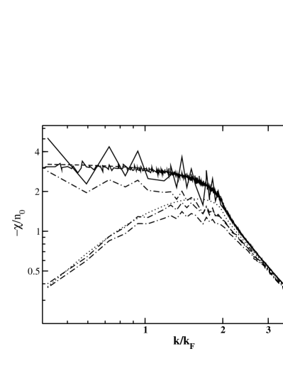
Figure 1: The dashed line shows the density response function $\chi_{0}$ of an infinitely large unpolarized non-interacting homogeneous electron gas (Lindhard function) at $r_{s}=2$. The black lines close to the Lindhard function show the exact finite-size Lindhard function $\chi_{0}^{fs}$with $114$ and $4218$ electrons, the latter following the Lindhard function closer. The dotted line shows the RPA response function $\chi_{RPA}$, and the three remaining dot-dashed lines show (from top to bottom) the fixed-node Lindhard function $\chi^{fn}_{0}$ at $114$ electrons, the corresponding fixed-node density response of an interacting system $\chi^{fn}$, and the fixed-node RPA $\chi_{RPA}^{fn}$. The “wiggles” are not noise as they correspond to the shell structure seen in the exact non-interacting finite-size $\chi_{0}^{fs}$

III.2 The density-response function

In general, the response function is given by

$$\chi_{AB}=\sum_{i=1}^{\infty}2\Re\frac{\langle 0|\hat{O}_{A}|i\rangle\langle i|\hat{O}_{B}|0\rangle}{E_{0}-E_{i}},$$ (9)

where the sum runs over all excited states of the many-electron system. fn DMC yields the ground-state energy for nodes given by the trial wave function. Therefore the second derivative yields the fixed-node response $\chi^{fn}$ of a system for which the nodes are the same for all perturbing potentials. Since in the case of a fixed-node system the sum entering Eq. (9) runs over a set of fixed-node excited states that differ from the actual excited states of the many-electron system, the fixed-node and non fixed-node non-interacting density-response function differ considerably (Fig. 1). Another interesting observation is the shell structure exhibited by all finite-size (fs) results. In order to visualize both the fixed-node error and the finite-size effects, we have plotted in Fig. 1 the following calculations: the static density-response function of (i) an infinitely large unpolarized non-interacting free electron gas, the well-known Lindhard function pines $\chi_{0}$ (dashed line), (ii) $\chi_{0}^{fs}$ of a non-interacting unpolarized system of 114 and 4218 electrons (solid lines), (iii) an infinitely large unpolarized interacting free electron gas in the random-phase approximation (RPA), $\chi_{RPA}$ (dotted line), (iv) a finite unpolarized system of 114 non-interacting electrons within the fixed-node approximation giving $\chi^{fn}_{0}$ (top dot-dashed line), (v) a finite unpolarized system of 114 interacting electrons within our fixed-node DMC scheme (middle dot-dashed line), and (vi) a finite unpolarized system of 114 interacting electrons in the fn RPA $\chi_{RPA}^{fn}$ (dot-dashed line at the bottom, see below for details). We see that the finite-size shell structure is not negligible even for a system of 4218 electrons. Nevertheless, the exact non-interacting density-response function nicely reproduces the well-known Lindhard function especially for $k/kf>2$.

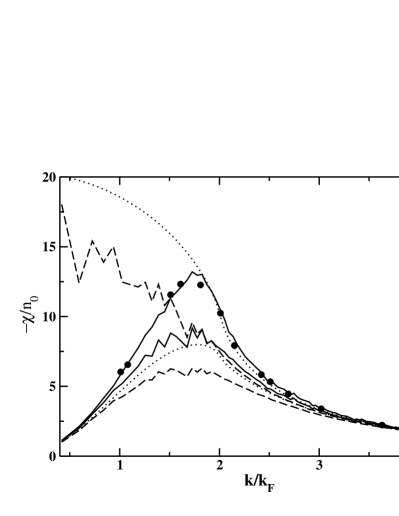
Figure 2: The density response at $r_{s}=5$ for an unpolarized $114$ particle homogeneous electron gas. The dotted lines show the Lindhard function $\chi_{0}$ (top) and $\chi_{RPA}$ (bottom). The dashed lines are $\chi_{0}^{fn}$ (top) and $\chi_{RPA}^{fn}$ (bottom). Finally, the solid lines show the fixed-node $\chi^{fn}$ (bottom) and extrapolated interacting $\chi$. The dots correspond to the results in Ref. cep . Our data reaches to smaller $k$ values as our system is larger ($114$ vs. up to $66$ electrons).

III.3 Discussion

Since the fn Lindhard function $\chi^{fn}_{0}$ (top dashed line in Fig. 2) is smaller than the real Lindhard function $\chi_{0}$ (dotted line at the top of Fig. 2) the fn interacting $\chi^{fn}$ is also too small (lower solid line in Fig. 2 compared to the dots showing the relevant data of Ref. cep ). However, assuming that the effect of the fixed-node nature of the calculation is the same for the interacting and non-interacting case, we should still be able to extract meaningful correlation data and reverse the effects of the fn approximation  fnrpa . Let us start with the definition for the exchange correlation (xc) kernel $f_{xc}$ and the local field factor $G$

$$-f_{xc}(k) = v_{C}(k)G(k)=\frac{1}{\chi(k)}-\frac{1}{\chi_{RPA}(k)}$$ (10)

$$= \frac{1}{\chi(k)}-\frac{1}{\chi_{0}(k)}+v_{C}(k)$$

where $v_{C}(k)=\frac{4\pi}{k^{2}}$. In practise, we do not have access to $\chi(k)$ but only to its finite-size equivalent in the fixed-node approximation. Moroni and coworkers  cep , who include the nodal variation at a Kohn-Sham level argue that that while the density response contains finite size effects, $f_{xc}$ is less afflicted by these. Hence, they extract $f_{xc}$ and add that back on to the non fixed-node infinite-cell Lindhard function to correct for finite size effects, thus eliminating the shell structure. There is no reason to expect the nodal variation of the KS nodes to correctly describe the nodal variation of the fully interacting system with respect to $\chi$: The KS nodes and the true many-body nodes are unrelated. Furthermore, different QMC systems at different numbers of electrons $N$ also correspond to distinct nodes, but the data for $f_{xc}$ (e.g. Ref. cep or Fig. 7) for different values of $N$ is mutually compatible. Finally, the effect of the nodal variation on $\chi_{0}$ seems universal, i.e. independent of $N$ except for shell effects (see Fig. 3).

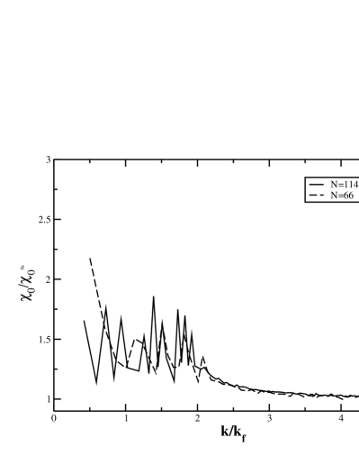
Figure 3: The ratio $\frac{\chi_{0}}{\chi_{0}^{fn}}$ at $r_{s}=5$ for $N=66$ and $N=114$ electrons. Due to scaling this graph is independent of the value of $r_{s}$, except for noise. Note the pronounced shell structure for $k<2k_{f}$.

It therefore seems reasonable to assume that $f_{xc}$ is independent of nodal effects and can thus be used to correct for wrong or absent nodal variation. Hence, by using the fixed-node quantities in Eq. (10), implicitly defining a fixed-node $\chi_{RPA}^{fn}$, we can derive a fn $f_{xc}^{fn}$ and $G^{fn}$ (Figures  4 and 5). These are remarkably similar to the data in Ref. cep . In fact, $f_{xc}^{fn}$ even has a slight dip as suggested in Ref. fxcref which however is not really visible in Ref. cep . This is encouraging and indeed we can use our data for $G^{fn}$ in conjunction with the real $\chi_{RPA}$ in Eq. (10) to estimate the non-fn interacting $\chi$. The result can be seen in Fig.  2: All the fn quantities are too small compared to their non-fn counterparts. However our extrapolated date (solid line at the top) is very close the extrapolated data of Ref. cep (dots).

For completeness sake Fig.  6 shows details of the extrapolated $\chi$ at $r_{s}=2$,$5$, and $10$. Also, in Fig. 7 we show a direct comparison between our results and Ref. cep where it is possible, i.e. at $N=66$ electrons in addition to our results for $N=114$ electrons confirming that all our data is compatible with Ref. cep . Except for noise there is no significant difference between data at different $N$, corroborating the assumption that $f_{xc}$ is independent of finite-size effects.

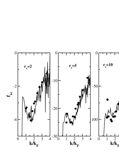
Figure 4: $f_{xc}^{fn}$ at $r_{s}=2,5,10$. The value at $k=0.4189k_{F}$ clearly is an outlier. Also, the noise increases as $k$ grows. Interestingly, there is a slight dip in $f_{xc}^{fn}$ for $k/k_{F}<2$ as demonstrated in Ref. fxcref . The dots correspond to the data in Ref. cep .

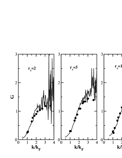
Figure 5: As figure 4, but showing the local field factor.

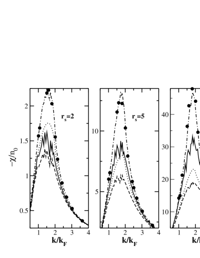
Figure 6: RPA (dotted), fn RPA (dashed), fn DMC (solid), and extrapolated (dot-dashed) density response function calculated using a $114$ particle homogeneous electron gas at $r_{s}=$ $2$,$5$, and $10$. The dots correspond to the results in Ref. cep . Note that for $r_{s}=2$ the uncorrected DMC data is lower still than standard RPA.

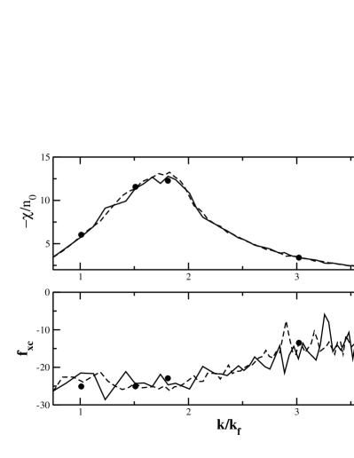
Figure 7: A comparison of our results for $f_{xc}$ at $r_{s}=5$ and the finite-size corrected $\chi$ with the data in Ref. cep where comparison is possible, i.e. at $N=66$ electrons. All our other data uses a larger simulation cell with $114$ electrons and more configurations in the DMC run. The solid dots are the four data points for $N=66$ electrons of Ref. cep and the solid line corresponds to our data (just under 100 data points in the shown region). The dashed line shows our data for the $N=114$ electron system. As suggested in Ref. cep there is no qualitative difference between $N=66$ and $N=114$. Note that for $N=66$ we use fewer walkers than for our main results at $N=114$.

In general, our results nicely follow the data in Ref. cep , who take into account the change in the nodes at a Kohn-Sham level, whereas our calculations do not take into account any nodal effect on xc quantities. The fact that the methods yield consistent results for $f_{xc}$ suggest that assuming $f_{xc}$ to be free from nodal effects is justified and that in either case the resulting data is an accurate description of systems with the full interacting nodal variation.

IV Concluding remarks

We have generalized Ref. hfs to the second derivative of the energy. This yields a novel method and an efficient algorithm to calculate the static response function within DMC. Our algorithm permits the computation of a large number of diagonal and off-diagonal terms in a single DMC run without the need for numerical derivatives or re-optimization. Noise can be efficiently controlled by increasing the number of DMC walkers and we have found that we can use large DMC time steps without introducing a bias, potentially speeding up calculations greatly. The wavefunction nodes have a strong effect on $\chi$, particularly for $k<3k_{F}$ and generalizing the RPA analysis using $\chi_{0}^{fn}$ yields a fixed-node $\chi_{RPA}^{fn}$. Using this to extract the xc contribution of $\chi$ we find that our method’s results are broadly in line with previous DMC calculations  cep which, however, are much more cumbersome, yield potentially fewer data points, and are effectively limited to diagonal terms only.

This work has been supported by the Basque Unibertsitate eta Ikerketa Saila and the Spanish Ministerio de Ciencia e Innovacion (Grants No. FIS2006-01343 and CSD2006-53). Computing facilities were provided by the Donostia International Physics Center (DIPC) and the SGI/IZO-SGIker UPV/EHU (supported by the National Program for the Promotion of Human Resources within the National Plan of Scientific Research, Development and Innovation-Fondo Social Europeo, MCyT and the Basque Government).

References

- (1) W. M. C. Foulkes, L. Mitas, R. J. Needs, and G. Rajagopal, Rev. Mod. Phys. 73, 33 (2001).
- (2) S. Moroni, D. M. Ceperley, and G. Senatore, Phys. Rev. Lett. 75, 689 (1995).
- (3) C Bowen, G. Sugiyama, and B. J. Alder, Phys. Rev. 50, 14838 (1994).
- (4) A. L. Fetter and J. D. Walecka, Quantum Theory of Many-Particle Systems, MgGraw-Hill, New York, 1971.
- (5) E. Runge and E. K. U. Gross, Phys. Rev. Lett. 52, 997 (1984).
- (6) R Gaudoin, J.M. Pitarke, Phys. Rev. Lett. 99, 126406 (2007).
- (7) R. P. Feynmann, Phys. Rev. 56, 340 (1939).
- (8) Note that the analysis leading to RPA (e.g. Ref. fetter ) does not mention nodes and thus should apply equally to the fn system.
- (9) Another method (J. Vrbik and S.M. Rothstein, J. Chem. Phys. 96, 2071 1992.) to calculate vibrational frequencies yields similar looking formulae. However, that method cannot be used for the exact fn sampling of general operators, only gives the fn response with respect to a parameter such as the distance between atoms, and applies specifically to DMC with fully retained weights.
- (10) R. J. Needs, M. Towler, N. Drummond, and P. Kent, CASINO version 1.7 User manual (University of Cambridge, 2004).
- (11) D. Pines and P. Noziers, The Theory of Quantum Liquids (Benjamin, New York, 1966).
- (12) B. Farid, V. Heine, G. E. Engel, and I. J. Robertson, Phys. Rev. B 48, 11602 (1993).