Momentum flow in black-hole binaries: II. Numerical simulations of equal-mass, head-on mergers with antiparallel spins.

Abstract

Research on extracting science from binary-black-hole (BBH) simulations has often adopted a “scattering matrix” perspective: given the binary’s initial parameters, what are the final hole’s parameters and the emitted gravitational waveform? In contrast, we are using BBH simulations to explore the nonlinear dynamics of curved spacetime. Focusing on the head-on plunge, merger, and ringdown of a BBH with transverse, antiparallel spins, we explore numerically the momentum flow between the holes and the surrounding spacetime. We use the Landau-Lifshitz field-theory-in-flat-spacetime formulation of general relativity to define and compute the density of field energy and field momentum outside horizons and the energy and momentum contained within horizons, and we define the effective velocity of each apparent and event horizon as the ratio of its enclosed momentum to its enclosed mass-energy. We find surprisingly good agreement between the horizons’ effective and coordinate velocities. During the plunge, the holes experience a frame-dragging-induced acceleration orthogonal to the plane of their spins and their infall (“downward”), and they reach downward speeds of order 1000 km/s. When the common apparent horizon forms (and when the event horizons merge and their merged neck expands), the horizon swallows upward field momentum that resided between the holes, causing the merged hole to accelerate in the opposite (“upward”) direction. As the merged hole and the field energy and momentum settle down, a pulsational burst of gravitational waves is emitted, and the merged hole has a final effective velocity of about 20 km/s upward, which agrees with the recoil velocity obtained by measuring the linear momentum carried to infinity by the emitted gravitational radiation. To investigate the gauge dependence of our results, we compare pseudospectral and moving-puncture evolutions of physically similar initial data; although spectral and puncture simulations use different gauge conditions, we find remarkably good agreement for our results in these two cases. We also compare our simulations with the post-Newtonian trajectories and near-field energy-momentum.

I Introduction

I.1 Motivation

Following Pretorius’s 2005 breakthrough Pretorius (2005a), several research groups have developed codes to solve Einstein’s equations numerically for the inspiral, merger, and ringdown of colliding binary black holes (BBHs). Most simulations of BBH mergers to date have adopted the moving-puncture method Campanelli et al. (2006); Baker et al. (2006a), and spectral methods Scheel et al. (2009) have also successfully simulated BBH mergers.

A major goal of current research is to successfully extract the physical content of these simulations. Typically, efforts toward this goal adopt a “scattering matrix” approach. Information obtained from numerical simulations on a finite set of islands in the seven-dimensional parameter space is being extrapolated, by various research groups, to design complicated functions that give the final parameters of the merged hole and the emitted gravitational waveforms as functions of the binary’s initial parameters.

In this paper, however, we take a different perspective: we focus our attention on the nonlinear dynamics of curved spacetime during the holes’ merger and ringdown. Following Ref. Keppel et al. (2009) (paper I in this series), our goal is to develop physical insight into the behavior of highly dynamical spacetimes such as the strong-field region near the black-hole horizons in a merging binary. As in paper I, we focus this study on the distribution and flow of linear momentum in BBH spacetimes. In contrast to paper I’s description of the pre-merger motion of the holes in the post-Newtonian approximation, in this paper we study the momentum flow during the plunge, merger, and ringdown of merging black holes in fully relativistic simulations.

I.2 Linear momentum flow in BBHs and gauge dependence

Typically, numerical simulations calculate only the total linear momentum of a BBH system and ignore the (gauge-dependent) linear momenta of the individual black holes. However, linear momentum has been considered by Krishnan, Lousto and Zlochower Krishnan et al. (2007). Inspired by the success of quasilocal angular momentum (see, e.g., Szabados (2004) for a review) as a tool for measuring the spin of an individual black hole, Krishnan and colleagues proposed an analogous (but gauge-dependent) formula for the quasilocal linear momentum, and they calculate this quasilocal linear momentum for, e.g., the highly-spinning, unequal-mass BBH simulations in Ref. Lousto and Zlochower (2009). This quasilocal linear momentum is also used to define an orbital angular momentum in Ref. Lousto and Zlochower (2008).

In this paper, we adopt a different, complementary method for measuring the holes’ linear momenta: for the first time, we apply the Landau-Lifshitz momentum-flow formalism (described in paper I and summarized in Sec. II) to numerical simulations of merging black holes. In this formalism, a mapping between the curved spacetime and an auxiliary flat spacetime (AFS) is chosen, and general relativity is reinterpreted as a field theory defined on this flat spacetime. The AFS has a set of translational Killing vectors which we use to define a localized, conserved linear momentum. In particular, we calculate i) a momentum density, ii) the momentum enclosed by horizons, and iii) the momentum enclosed by distant coordinate spheres. In the asymptotically flat region around a source, there is a preferred way to choose the mapping between the curved spacetime and the AFS; consequently, in this limit item iii) is gauge-invariant. In general, though, the choice of mapping is arbitrary, and it follows that items i) and ii) are necessarily gauge-dependent.

By examining the linear momentum flow in a dynamical spacetime—and living with the inevitable gauge dependence—we hope to develop strong intuition for the behavior of BBHs. As in paper I, we envision different numerical relativity groups choosing “preferred” gauges based on the coordinates of their numerical simulations. While there is no reason, a priori, why simulations in different gauges should agree, one of our hopes from paper I is realized for the cases we consider; namely, in this paper, we calculate the horizon-enclosed momentum using spectral and moving-puncture evolutions of similar initial data, and we do find surprisingly good agreement (cf. Figs. 8 and 15), even though the simulations use manifestly different gauge conditions [Eqs. (14) for the spectral simulations and Eqs. (50)–(51) for the puncture simulations]. These are two of the most commonly used gauge conditions in numerical relativity.

Therefore, we continue to hope that in general—for the gauges commonly used in numerical simulations—the momentum distributions for evolutions of physically similar initial data will turn out to be at least qualitatively similar. If further investigation reveals this to be the case, then different research groups can simply use the coordinates used in the their simulations as the “preferred coordinates” for constructing the mapping to the AFS. Otherwise, we would advocate (as in Sec. I C of paper I) that different numerical-relativity groups construct the mapping to the AFS by first agreeing on a choice of “preferred” coordinates (e.g., a particular harmonic gauge) and then transforming the results of their simulations to those coordinates.

I.3 BBH mergers with recoil

A particularly important application of this approach is an exploration of the momentum flow in BBH mergers with recoil. The gravitational recoil or kick effect arising in a BBH coalescence has attracted a great deal of attention in recent years in the context of a variety of astrophysical scenarios including the structure of galaxies Boylan-Kolchin et al. (2004); Gualandris and Merritt (2008); Komossa and Merritt (2008), the reionization history of the universe Madau et al. (2004), the assembly of supermassive black holes Haiman (2004); Madau and Quataert (2004); Merritt et al. (2004); Volonteri (2007); Blecha and Loeb (2008) and direct observational signatures Loeb (2007); Komossa et al. (2008); Menou et al. (2008). For a long time, estimates of the recoil magnitude were based on approximative techniques Fitchett (1983); Favata et al. (2004); Blanchet et al. (2005); Damour and Gopakumar (2006); accurate calculations in the framework of fully nonlinear general relativity have only become possible in the aftermath of important breakthroughs in the field of numerical relativity Pretorius (2005a); Campanelli et al. (2006); Baker et al. (2006a).

Several groups have used numerical simulations to study the kick resulting from the merger of non-spinning and spinning binaries (see, e.g., Baker et al. (2006b); Gonzalez et al. (2007a); Herrmann et al. (2007); Koppitz et al. (2007); Campanelli et al. (2007a); Tichy and Marronetti (2007)). Most remarkably, recoil velocities of several thousand km/s have been found for binaries with equal and opposite spins in the orbital plane Campanelli et al. (2007a); Gonzalez et al. (2007b); Campanelli et al. (2007b), and variants thereof with hyperbolic orbits even generate $10^{4}~{}{\rm km/s}$ Healy et al. (2008). Given the enormous astrophysical repercussions of such large recoil velocities, the community is now using various approaches to obtain a better understanding of the kick as a function of the initial BBH parameters Boyle et al. (2008); Boyle and Kesden (2008); Schnittman and Buonanno (2007); Baker et al. (2008); Tichy and Marronetti (2008); Lousto et al. (2009) resulting in phenomenological fitting formulas; see Baker et al. (2007); Lousto and Zlochower (2008); Baker et al. (2008); Gonzalez et al. (2009); Rezzolla (2009); Lousto and Zlochower (2009) and references therein.

On the other hand, our understanding of the local dynamics in these extraordinarily violent events is still rather limited. Some insight into the origin of the holes’ kick velocity has been obtained by examining the individual multipole moments of the emitted gravitational waves Schnittman et al. (2008); Miller and Matzner (2009) and by approximating the recoil analytically using post-Newtonian Blanchet et al. (2005); Racine et al. (2008), effective-one-body Damour and Gopakumar (2006), and black-hole-perturbation theory Mino and Brink (2008). An intuitive picture describing aspects of the so-called superkick configurations generating velocities in the thousands of km/s has been given in terms of the frame-dragging effect (cf. Fig. 5 of Ref. Pretorius (2007)).

Investigating the momentum distribution and flow in recoiling BBH mergers could help to build further intuition into the nonlinear dynamics of the spacetime and their influence on the formation of kicks. Paper I made some headway into the former issue but could not address the latter. Specifically, paper I examined the distribution and the flow of linear momentum in BBH spacetimes using the Landau-Lifshitz formalism in the post-Newtonian approximation. It then specialized this approach to the extreme-kick configuration Campanelli et al. (2007a); Gonzalez et al. (2007b); Campanelli et al. (2007b), which is a system of inspiraling, BBHs with equal and anti-parallel spins in the orbital plane. During inspiral, the two black holes simultaneously and sinusoidally bob perpendicularly to the orbital plane; in paper I, this motion was first recognized as arising from the combined effect of frame dragging and spin-curvature coupling and then was found to arise from the exchange of momentum between the near-zone gravitational field and the black holes.

Because paper I analyzed the system at a post-Newtonian level, its analysis could not be extended to merger and beyond. Consequently, it was not possible to address how the nonlinear dynamics in the pre-merger near zone transitions into the final behavior of the merged black hole. This paper (paper II) lets us begin to address this transition as we study momentum flow during the plunge, merger, and ringdown of BBHs in full numerical relativity. Our study allows us, for example, to examine how accurately Pretorius’s intuitive picture applies during the merger and ringdown of a recoiling BBH merger.

I.4 Overview and summary

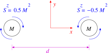
Figure 1: Initial configuration of the head-on BBH considered in this paper. The holes move primarily along the $x$ axis, but they also accelerate in the $-y$ (downward) direction due to frame dragging. See Table 1 for the value of $d=2x_{0}$.

As a first step toward analyzing the momentum flow in superkicks, in this paper we apply the Landau-Lifshitz momentum-flow formalism to a much simpler case: the head-on plunge, merger, and ringdown of an equal-mass BBH. The holes initially have antiparallel spins of equal magnitude that are transverse to the holes’ head-on motion (Fig. 1). Primarily, the holes simply fall toward each other in the $\pm x$ direction. However, each hole’s spin drags the space around itself, causing the other hole to accelerate in the downward, $-y$ direction.

How does this frame dragging relate to the final kick velocity of the merged hole? To address this question, we compute the 4-momentum $p^{\mu}$ inside each apparent horizon using the Landau-Lifshitz formalism; we then define an effective velocity as

$$v^{i}_{\rm LL}:=\frac{p^{i}}{p^{0}}.$$ (1)

In Sec. IV, we find that this effective velocity behaves similarly to the horizons’ coordinate velocities.

The effective $y$ velocity for the spectral simulation described in Sec. III.1.2 is shown in Fig. 2. Before the merger, the individual apparent horizons do indeed accelerate in the $-y$ (“down”) direction, eventually reaching velocities of order $10^{3}$ km/s. However, when the common apparent horizon forms, it pulsates; during the first half-pulsation, the horizon expands and accelerates to $\sim 10^{3}$ km/s in the up ($+y$) direction. This happens because as the common horizon forms and expands, it swallows not only the downward linear momentum inside each individual horizon but also a large amount of upward momentum in the gravitational field between the holes (Fig. 3). During the next half-pulsation, as the horizon shape changes from oblate to prolate (cf. Fig. LABEL:fig:Shape), the horizon swallows a net downward momentum, thereby losing most of its upward velocity. Eventually, after strong damping of the pulsations, the common horizon settles down to a very small velocity of about 23 km/s in the $+y$ direction (inset of Fig. 2), which (Sec. IV) is consistent with the kick velocity inferred from the emitted gravitational radiation.

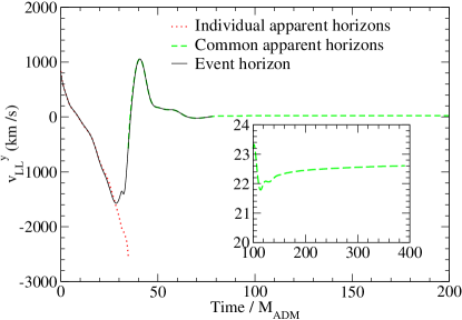
Figure 2: The effective velocity $v^{y}_{\rm LL}$ for the individual (red dotted line) and common (green dashed line) apparent horizons and for the event horizon (black solid line). The inset shows the velocity of the common apparent horizon at late times.

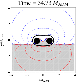
Figure 3: A contour plot of the $y$ component of the momentum density at the moment when the common apparent horizon forms. The common horizon encloses the momentum inside the individual horizons and also the momentum in the gravitational field. The grey-shaded region and solid, red contours indicate positive momentum density, while the white-shaded region and blue, dashed contours indicate negative momentum density. The individual apparent horizons are shaded black, and the common apparent horizon is shown as a thick black line.

This momentum flow between field and holes is also described quite beautifully in the language of the holes’ event horizon. Unlike apparent horizons, the event horizon evolves and expands continuously in time, rather than discontinuously. As the event horizon expands, it continuously swallows surrounding field momentum, and that swallowing produces a continuous evolution of the event horizon’s velocity, an evolution that is nearly the same as for the apparent-horizon velocity. Figure 2 shows how the effective velocity of the event horizon smoothly transitions from matching the individual apparent horizons’ velocities to matching the common apparent horizon’s velocity. For further details, see Sec. IV.1.2 and especially Figs. 13 and 14.

In the remainder of this paper, we discuss our results and the simulations that are used to obtain them. In Sec. II, we briefly review the Landau-Lifshitz formalism and momentum conservation. The simulations themselves are presented in Sec. III. We analyze the simulations’ momentum flow in Sec. IV and conclude in Sec. V. In the appendices, we describe in greater depth the numerical methods used for the simulations presented in this paper.

II 4-Momentum Conservation in the Landau-Lifshitz Formalism

In this section, we briefly review the Landau-Lifshitz formulation of gravity and the statement of 4-momentum conservation within this theory. Landau and Lifshitz, in their Classical Theory of Fields (hereafter referred to as LL), reformulated general relativity as a nonlinear field theory in flat spacetime Landau and Lifshitz (1962). (Chap. 20 of MTW Misner et al. (1973) and a paper by Babak and Grishchuk Babak and Grishchuk (1999) are also helpful sources that describe the formalism.) Landau and Lifshitz develop their formalism by first laying down arbitrary asymptotically Lorentz coordinates on a given curved (but asymptotically-flat) spacetime. They use these coordinates to map the curved (i.e. physical) spacetime onto an auxiliary flat spacetime (AFS) by enforcing that the coordinates on the AFS are globally Lorentz. The auxiliary flat metric takes the Minkowski form, $\eta_{\mu\nu}={\rm diag}(-1,1,1,1)$.

In this formulation, gravity is described by the physical metric density

$$\mathfrak{g}^{\mu\nu}:=\sqrt{-g}g^{\mu\nu}\;,$$ (2)

where $g$ is the determinant of the covariant components of the physical metric, and $g^{\mu\nu}$ are the contravariant components of the physical metric. When one defines the superpotential

$$H^{\mu\alpha\nu\beta}:=\mathfrak{g}^{\mu\nu}\mathfrak{g}^{\alpha\beta}-\mathfrak{g}^{\mu\alpha}\mathfrak{g}^{\nu\beta}\;,$$ (3)

the Einstein field equations take the field-theory-in-flat-spacetime form

$${H^{\mu\alpha\nu\beta}}_{,\alpha\beta}=16\pi\tau^{\mu\nu}\;.$$ (4)

Here $\tau^{\mu\nu}:=(-g)(T^{\mu\nu}+t^{\mu\nu}_{\rm LL})$ is the total effective stress-energy tensor, indices after the comma denote partial derivatives or, equivalently, covariant derivatives with respect to the flat auxiliary metric), and the Landau-Lifshitz pseudotensor $t^{\mu\nu}_{\rm LL}$ (a real tensor in the auxiliary flat spacetime) is given by Eq. (100.7) of LL Landau and Lifshitz (1962) or equivalently Eq. (20.22) of MTW Misner et al. (1973):

$$16\pi(-g)t^{\alpha\beta}_{\rm LL} = \mathfrak{g}^{\alpha\beta}{{}_{,\lambda}}\mathfrak{g}^{\lambda\mu}{{}_{,\mu}}-\mathfrak{g}^{\alpha\lambda}{{}_{,\lambda}}\mathfrak{g}^{\beta\mu}{{}_{,\mu}}$$ (5)

$$+ \frac{1}{2}g^{\alpha\beta}g_{\lambda\mu}\mathfrak{g}^{\lambda\nu}{{}_{,\rho}}\mathfrak{g}^{\rho\mu}{{}_{,\nu}}$$

$$- g^{\alpha\lambda}g_{\mu\nu}\mathfrak{g}^{\beta\nu}{{}_{,\rho}}\mathfrak{g}^{\mu\rho}{{}_{,\lambda}}-g^{\beta\lambda}g_{\mu\nu}\mathfrak{g}^{\alpha\nu}{{}_{,\rho}}\mathfrak{g}^{\mu\rho}{{}_{,\lambda}}$$

$$+ g_{\lambda\mu}g^{\nu\rho}\mathfrak{g}^{\alpha\lambda}{{}_{,\nu}}\mathfrak{g}^{\beta\mu}{{}_{,\rho}}$$

$$+ \frac{1}{8}\left(2g^{\alpha\lambda}g^{\beta\mu}-g^{\alpha\beta}g^{\lambda\mu}\right)$$

$$\times \left(2g_{\nu\rho}g_{\sigma\tau}-g_{\rho\sigma}g_{\nu\tau}\right)\mathfrak{g}^{\nu\tau}{{}_{,\lambda}}\mathfrak{g}^{\rho\sigma}{{}_{,\mu}}$$

Due to the symmetries of the superpotential—they are the same as those of the Riemann tensor—the field equations (4) imply the differential conservation law for 4-momentum

$${\tau^{\mu\nu}}_{,\nu}=0\;.$$ (6)

Eq. (6) is equivalent to ${T^{\mu\nu}}_{;\nu}=0$, where the semicolon denotes a covariant derivative with respect to the physical metric.

In both LL and MTW, it is shown that the total 4-momentum of any isolated system (measured in the asymptotically flat region far from the system) is

$$p^{\mu}_{\rm tot}=\frac{1}{16\pi}\oint_{\mathcal{S}}{H^{\mu\alpha 0j}}_{,\alpha}d\Sigma_{j}\;,$$ (7)

where $d\Sigma_{j}$ is the surface-area element of the flat auxiliary metric, and $\mathcal{S}$ is an arbitrarily large surface surrounding the system. This total 4-momentum satisfies the usual conservation law

$$\frac{dp^{\mu}_{\rm tot}}{dt}=-\oint_{\mathcal{S}}\tau^{\mu j}d\Sigma_{j}\;.$$ (8)

See the end of Section III of Keppel et al. (2009) for a brief proof of why this holds for black holes.

Because this paper focuses on BBHs, we will make a few further definitions that will be used frequently in our study. First, we label the two black holes in the binary (and the regions of space within their horizons) by $A$ and $B$, and denote their surfaces (sometimes the hole’s event horizon and other times the apparent horizon) by $\partial A$ and $\partial B$, as shown in Fig. 4. We let $\mathcal{E}$ stand for the region outside both bodies but inside the arbitrarily large surface $\mathcal{S}$ where the system’s total momentum is computed (in our case, this is taken to be a fixed coordinate sphere inside the outer boundary of the numerical-relativity computational grid).

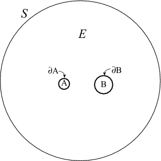
Figure 4: The regions of space around and inside a binary-black-hole system.

With the aid of Gauss’s theorem and the Einstein field equations (4), one can reexpress Eq. (7) for the binary’s total 4-momentum as a sum over contributions from each of the bodies and from the gravitational field in the region $\mathcal{E}$ outside them:

$$p_{\rm tot}^{\mu}=p_{A}^{\mu}+p_{B}^{\mu}+p_{\rm field}^{\mu}\;.$$ (9a)

Here

$$p_{A}^{\mu}:=\frac{1}{16\pi}\oint_{\partial A}{H^{\mu\alpha 0j}}_{,\alpha}d\Sigma_{j}$$ (9b)

is the 4-momentum of body $$A B$$ (an equivalent expression holds for body ), and

$$p_{\rm field}^{\mu}:=\int_{\mathcal{E}}\tau^{0\mu}d^{3}x$$ (9c)

is the gravitational field’s 4-momentum in the exterior of the black holes.

We define an effective velocity of black hole $A$ (with similar expressions holding for hole $B$) by

$$v_{\rm LL}^{j}:=\frac{p^{j}_{A}}{p^{0}_{A}}\;.$$ (10)

In analogy to Eq. (8) for the rate of change of the binary’s total 4-momentum, one can write the corresponding equation for the rate of change of the 4-momentum of body $A$:

$$\frac{dp^{\mu}_{A}}{dt}=-\oint_{\partial A}(\tau^{\mu k}-\tau^{\mu 0}v^{k}_{A})d\Sigma_{k}\;.$$ (11)

Equation (11) describes the flow of field 4-momentum into and out of body $A$ (the second term comes from the motion of the boundary of body $A$ with local coordinate velocity $v^{k}_{A}$).

We will use Eqs. (8)–(10) as the basis for our study of momentum flow in black-hole binaries. The actual values of the body and field 4-momenta, computed in the above ways, will depend on the arbitrary mapping between the physical spacetime and the AFS; this is the gauge-dependence that will be discussed in Sec. IV.2.

III Simulations of head-on BBH collisions with anti-aligned spins

In order to investigate the gauge dependence of our results, we compare simulations of the same physical system using two separate methods that employ different choices of coordinates. One method is a pseudospectral excision scheme based on generalized harmonic coordinates; the other is a finite-difference moving-puncture scheme that uses 1+log slicing and a gamma-driver shift condition (henceforth referred to as “moving puncture gauge”; for details see Appendix B.2). The coordinates used in the two methods differ both for the initial data and during the evolution. In this section we summarize the construction of initial data and the evolution scheme for both methods, and we present convergence tests and estimate numerical uncertainties. Further details about our numerical methods are are given in Appendices A and B.

III.1 Pseudospectral

III.1.1 Quasiequilibrium excision data

The evolutions described in Sec. III.1.2 begin with quasiequilibrium excision data constructed using the method of Ref. Lovelace et al. (2008). This method requires the arbitrary choice of a conformal three-metric; we choose this metric to be flat almost everywhere but curved (such that the metric is nearly that of a single Kerr-Schild hole) near the horizons.

Our initial data method also requires us to choose an outer boundary condition on a shift vector $\beta^{i}$; for a general binary that is orbiting and inspiraling, we use

$$\beta^{i}=\left(\mathbf{\Omega}_{0}\times r\right)^{i}+\dot{a}_{0}r^{i}+V_{0}^{i},\mbox{ }r\rightarrow\infty,$$ (12)

where $\Omega_{0}$ is the angular velocity, $\dot{a}_{0}r^{i}$ is the initial radial velocity, and $V_{0}^{i}$ is a translational velocity. Note that Eq (12) is different from the choice made in Ref. Lovelace et al. (2008). In this paper we confine our focus to collisions that are head-on, which we define as $\Omega_{0}=\dot{a}_{0}=0$. However, $V_{0}^{i}$ must be nonzero to make the total linear momentum of the initial data vanish.

Table 1 summarizes the initial data used in this paper. The Arnowitt-Deser-Misner (ADM) mass $M_{\rm ADM}$ (Eq. (11.2.14) in Ref. Wald (1984); see also Arnowitt et al. (1962); York, Jr. (1979)), the irreducible mass $M_{\rm irr}$ and Christodoulou mass $M_{\rm Chr}$ of one of the holes are listed, where $M_{\rm Chr}$ is related to $M_{\rm irr}$ and the spin of the hole $S_{z}$ by

$$M_{\rm Chr}^{2}=M_{\rm irr}^{2}+\frac{S_{z}^{2}}{4M_{\rm irr}^{2}}.$$ (13)

Table 1 also shows the dimensionless spin $S_{z}/M_{\rm Chr}^{2}$; by definition, this measure of the spin lies in the interval $-1\leq S_{z}/M_{\rm Chr}^{2}\leq 1$.

For set S1 listed in Table 1, $V_{0}^{i}$ is adjusted so that the initial effective velocity of the entire spacetime $v^{i}_{\rm tot}:=p^{i}_{\rm tot}/p^{0}_{\rm tot}$ is smaller than 0.1 km/s, which is approximately the size of our numerical truncation error (cf. Fig. 9): $\left(\left|v^{x}_{\rm tot}\right|,\left|v^{y}_{\rm tot}\right|,\left|v^{z}_{\rm tot}\right|\right)=(4\times 10^{-4},5\times 10^{-2},2\times 10^{-3})$ km/s at time $t=0$.

The construction of initial data is described in more detail in Appendix A.

Set	$x_{o}/M_{\rm ADM}$	$M_{\rm irr}/M_{\rm ADM}$	$M_{\rm Chr}/M_{\rm ADM}$	$S_{z}/M_{\rm Chr}^{2}$
S1	$3.902$	0.4986	0.5162	$\pm 0.5000$
P1	$4.211$	0.4970	0.5146	$\pm 0.5000$
P2	$8.368$	0.4802	0.5072	$\pm 0.5091$
H1	$14.864$	0.4870	0.5042	$\pm 0.5000$

Table 1: Parameters of the initial data configurations studied in this work. Model S1 (see Sec. III.1.1) gives the parameters used to construct a set of Superposed-Kerr-Schild quasiequilibrium excision initial data. Model H1 (see Appendix D) gives the parameters for the larger separation Superposed-Harmonic-Kerr initial data set. Both S1 and H1 were used in spectral evolutions. P1 and P2 provide the Bowen-York parameters for the two systems evolved with the moving puncture method. The holes are initially separated by a coordinate distance $d=2x_{0}$ and are located at coordinates $(x,y,z)=(\pm x_{0},0,0)$. For clarity, only 4 significant figures are shown.

III.1.2 Generalized harmonic evolutions

We evolve the quasiequilibrium excision data described in Sec. III.1.1 pseudospectrally, using generalized harmonic gauge Friedrich (1985); Garfinkle (2002); Pretorius (2005b); Lindblom et al. (2006), for which the coordinates $x^{\mu}$ satisfy the gauge condition

$$g_{\mu\nu}\nabla^{\rho}\nabla_{\rho}x^{\mu}=H_{\nu}\left(x^{\rho},g_{\sigma\tau}\right)$$ (14)

where $H_{\nu}$ is a function of the coordinates and the spacetime metric. In this subsection, we summarize the computational grid used for our spectral evolutions, and we briefly discuss our numerical accuracy. Details of our pseudospectral evolutions are given in Appendix B.1.

Our computational grid covers only the exterior regions of the black holes (“black hole excision”): there is an artificial inner boundary just inside each apparent horizon where no boundary condition is needed because of causality. The grid extends to a large radius $r_{\rm max}\sim 400M_{\rm ADM}$. A set of overlapping subdomains of different shapes (spherical shells near each hole and far away; cylinders elsewhere) covers the entire space between the excision boundaries and $r=r_{\rm max}$.

Because different subdomains have different shapes and the grid points are not distributed uniformly, we describe the resolution of our grid in terms of the total number of grid points summed over all subdomains. We label our resolutions $\mbox{N}0$, $\mbox{N}1$, and $\mbox{N}2$, corresponding to approximately $55^{3}$, $67^{3}$, and $79^{3}$ grid points, respectively. After merger, we regrid onto a new computational domain that has only a single excised region (just inside the newly-formed apparent horizon that encompasses both holes). This new grid has a different resolution (and a different decomposition into subdomains) from the old grid. We label the resolution of the post-merger grid by $A$, $B$, and $C$, corresponding to approximately $63^{3}$, $75^{3}$, and $87^{3}$ gridpoints, respectively. We label the entire run using the notation ‘N$x$.$y$’, where the characters before and after the decimal point denote the pre-merger and post-merger resolution for that run. Thus, for example, ‘$\mbox{N}2.B$’ denotes a run with approximately $67^{3}$ grid points before merger, and $75^{3}$ grid points afterward. On the outermost portion of the grid (farther than $\sim 200M_{\rm ADM}$), we use a coarser numerical resolution than we do elsewhere. (We only measure the gravitational wave flux, linear momentum, etc., at radii of $r\leq 160M_{\rm ADM}$.)

To demonstrate the convergence of our evolutions, we plot the constraint violation in Fig. 5 for several resolutions. The quantity plotted is the $L^{2}$ norm of all the constraints of the generalized harmonic system, normalized by the $L^{2}$ norm of the spatial gradients of all the dynamical fields, as defined by by Eq. (71) of Ref. Lindblom et al. (2006). The left portion of the plot depicts the constraint violation during the plunge, the right third of the plot shows the constraint violation during the ringdown, and the middle panel shows the constraints shortly before and shortly after the common apparent horizon forms. Throughout the evolution, we generally observe exponential convergence, although the convergence rate is smaller near merger. After merger, there are two sources of constraint violations: those generated by numerical truncation error after merger (these depend on the resolution of the post-merger grid) and those generated by numerical truncation error before merger and are still present in the solution (these depend on the resolution of the pre-merger grid). We see from Fig. 5 that the constraint violations after merger are dominated by the former source. Also, at about $t=200M_{\rm ADM}$, the constraint violation increases noticeably (but is still convergent); at this time, the outgoing gravitational waves have reached the coarser, outermost region of the grid.

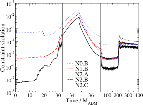
Figure 5: Constraint violation at different numerical resolutions for the pseudospectral evolutions S1. The common apparent horizon forms at time $t=34.73M_{\rm ADM}$. Labels of the form $\mbox{N}x.y$ indicate the grid resolution, where the pre-merger resolution is labeled (from coarse to fine) by $x=0,1,2$ and the post-merger resolution is labeled by $y=A,B,C$. The constraints decrease exponentially with higher resolution; the convergence rate is smaller near merger.

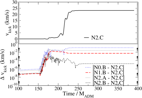
Figure 6: Recoil velocity for initial data set S1 inferred from the gravitational wave signal $\Psi_{4}$ extracted at $r_{\rm extr}=160M_{\rm ADM}$ at the highest resolution (upper panel). Differences between several coarser resolutions and the highest resolution result are plotted in the lower panel.

Finally, in Fig. 6, we demonstrate the accuracy of the recoil velocity $v_{\rm kick}=22$ km/s inferred from the gravitational wave signal $\Psi_{4}$, which asymptotically is related to the gravitational wave amplitudes $h_{+}$ and $h_{\times}$ by

$$\Psi_{4}=\frac{d^{2}}{dt^{2}}h_{+}-i\frac{d^{2}}{dt^{2}}h_{\times}.$$ (15)

We extract the spin-weighted spherical harmonic coefficients of $\Psi_{4}(t)$ from the simulation as described in Ref. Scheel et al. (2009), and we integrate these coefficients over time to obtain $\dot{h}^{\ell m}(t)$, which are the spin-weighted spherical harmonic coefficients of $\dot{h}=\dot{h}_{+}-i\dot{h}_{\times}$. For each $(\ell,m)$, the integration constant is chosen so that the average value of $\dot{h}^{\ell m}(t)$ is zero. The $\dot{h}^{\ell m}(t)$ are then used to compute the 4-momentum flux of the gravitational waves from Eqs. (3.14)–(3.19) of Ref. Ruiz et al. (2008). Integrating this flux over time yields the total radiated energy-momentum, $p^{\mu}_{\rm rad}$. The recoil velocity can then be computed from energy-momentum conservation: $v^{i}_{\rm kick}=-p^{i}_{\rm rad}/M_{\rm final}$, where $M_{\rm final}:=M_{\rm ADM}-E_{\rm rad}$ and $E_{\rm rad}$ is the energy radiated to infinity. For set S1, we obtain a radiated energy of $E_{\rm rad}/M_{\rm ADM}=(5.6840\pm 0.0008)\times 10^{-4}$, where the quoted error includes truncation error and uncertainty from extrapolation to infinite radius (as discussed below). The top panel of Fig. 6 shows the recoil velocity as a function of time for our highest resolution simulation, while the lower panel shows differences between the highest resolution ($\mbox{N}2.C$) and lower resolutions. From these differences, we estimate a numerical uncertainty for the final recoil velocity of $5\times 10^{-3}$ km/s for $\mbox{N}1.B$ and $2\times 10^{-5}$ km/s for $\mbox{N}2.B$.

This numerical uncertainty includes only the effects of numerical truncation error; however, there are other potential sources of uncertainty in the simulations that must also be considered. The first is the spurious “junk” gravitational radiation that arises because the initial data do not describe a perfect equilibrium situation. This radiation is not astrophysically realistic, but by carrying a small amount of energy-momentum that contributes to the measured $p^{\mu}_{\rm rad}$ at large distances, the spurious radiation does affect our determination of the final recoil velocity. In our investigation of momentum flow (Sec. IV), we do not correct for the initial data’s failure to be in equilibrium; here we estimate the contribution of the resulting spurious radiation to the final recoil velocity. First, we note that for head-on collisions, the physical gravitational waves are emitted predominantly after merger. Therefore, we estimate the influence of the spurious radiation by examining the accumulated recoil velocity at time $t=\Delta t+r$, where $r$ is the radius of the extraction surface and $\Delta t$ is a cutoff time. Because the holes merge so quickly (because they begin at so small an initial separation), the spurious and physical contributions to the recoil are not clearly distinguishable in Fig. 6. Varying $\Delta t$ between $31.1M_{\rm ADM}$ and $38.3M_{\rm ADM}$ (the common event and apparent horizons form at $t=31.1M_{\rm ADM}$ and $t=34.7M_{\rm ADM}$, respectively), we estimate that the spurious radiation contributes approximately $1$ km/s (about 5%) to the recoil velocity—a much larger uncertainty than the truncation error. The same variation of $\Delta t$ implies that the spurious radiation contributes about 10% of the total radiated energy $E_{\rm rad}$.)

Another potential source of uncertainty in $v^{i}_{\rm kick}$ arises from where on the grid we measure the gravitational radiation. In particular, the quantity $\Psi_{4}$ in Eq. (15) should ideally be measured at future null infinity. Instead, we measure $\Psi_{4}$ on a set of coordinate spheres at fixed radii, compute $v^{i}_{\rm kick}$ on each of these spheres, and extrapolate the final equilibrium value of $v^{i}_{\rm kick}$ to infinite radius. The dotted curves on Fig. 12 show $v^{y}_{\rm kick}$ measured from $\Psi_{4}$ at several radii, and the black cross shows the final value of $v^{y}_{\rm kick}$ extrapolated to infinity. We estimate our uncertainty in the extrapolated value by comparing polynomial extrapolation of orders $1$, $2$, and $3$; we find an uncertainty of $3\times 10^{-3}$ km/s for the quadratic fit. Note that if we had not extrapolated to infinity, but had instead simply used the value of $v^{y}_{\rm kick}$ at our largest extraction sphere ($r=160M_{\rm ADM}$), we would have made an error of $0.85$ km/s, which is much larger than the uncertainty from numerical truncation error. Finally, we mention that our computation of $\Psi_{4}$ is not strictly gauge invariant unless $\Psi_{4}$ is evaluated at future null infinity. As long as gauge effects in $\Psi_{4}$ fall off faster than $1/r$ as expected, extrapolation of $v^{y}_{\rm kick}$ to infinity should eliminate this source of uncertainty.

III.2 Moving puncture

III.2.1 Bowen-York puncture data

In order to address the importance of gauge dependence for our calculations using the Landau-Lifshitz formalism, we also simulate BBH mergers using the so-called moving puncture method, which employs the covariant form of “1+log” slicing Campanelli et al. (2006); Bona et al. (1997) for the lapse function $\alpha$ and a “Gamma-driver” condition (based on the original “Gamma-freezing” condition introduced in Alcubierre et al. (2003a)) for the shift vector. The precise evolution equations for the gauge variables as well as further technical details of our puncture simulations are given in Appendix B.2.

Our simulations start with puncture initial data Brandt and Brügmann (1997) provided in our case by the spectral solver of Ref. Ansorg et al. (2004). The initial data are fully specified in terms of the initial spin $\vec{S}_{1,2}$, linear momentum $\vec{P}_{1,2}$ and initial coordinate position $\vec{x}_{1,2}$ as well as the bare mass parameters $m_{1,2}$ of either hole Bowen and York, Jr. (1980). The corresponding nonvanishing values for the two puncture models considered in this work are given in Table 1. There we also list the total black-hole mass $M_{\rm Chr}$ and normalize all quantities using the total ADM mass $M_{\rm ADM}$. The main difference between the two configurations is the initial separation of the holes. The lapse and shift are initialized as $\alpha=\gamma^{-1/6}$ and $\beta^{i}=0$, where $\gamma$ is the determinant of the physical three-metric.

III.2.2 Moving puncture evolutions

The evolution of the puncture initial data is performed using sixth order spatial discretization of the BSSN equations combined with a fourth order Runge-Kutta time integration. Mesh refinement of Berger-Oliger Berger and Oliger (1984) type is implemented using Schnetter’s Carpet package Schnetter et al. (2004); Car . The prolongation operator is of fifth order in space and quadratic in time. Outgoing radiation boundary conditions are implemented using second-order accurate advection derivatives (see, for example, Sec. VI in Ref. Alcubierre et al. (2003b)).

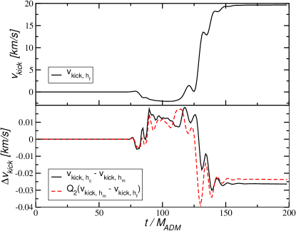
Figure 7: Gravitational recoil for model P1 as estimated from the gravitational wave signal $\Psi_{4}$ extracted at $r_{\rm ex}=73.5~{}M_{\rm ADM}$ using the highest resolution (upper panel). Differences in the recoil obtained at coarse, medium and fine resolution rescaled for second order convergence (lower panel).

Using the notation of Sec. II E of Ref. Sperhake (2007) the grid setup in units of $M_{\rm ADM}$ for these evolutions is given by (rounded to 3 significant digits)

$$\{(202,101,58.8,25.2,12.6)\times(3.15,1.58,0.788),~{}h\},$$

$$\{(201,100,58.5,25.1)\times(6.27,3.13,1.57,0.784),~{}h\},$$

respectively. Here $h$ denotes the resolution on the innermost refinement level. For model P1 we perform a convergence analysis by setting $h$ to $h_{\rm c}=M_{\rm ADM}/49.5$, $h_{\rm m}=M_{\rm ADM}/57.1$ and $h_{\rm f}=M_{\rm ADM}/64.7$, respectively, for coarse, medium and fine resolution. Model P2 is evolved using $h=M_{\rm ADM}/49.8$.

Before we discuss the physical results from the puncture simulations, we estimate the numerical errors due to discretization, finite extraction radius and the presence of unphysical gravitational radiation in the initial data.

In order to study the dependence of the results on resolution, we have evolved model P1 of Table 1 using different resolutions $h_{\rm c}$, $h_{\rm m}$ and $h_{\rm f}$ on the finest level and correspondingly larger grid spacings by a factor of two on each consecutive level. The kick velocity from the high resolution simulation, as inferred from the gravitational radiation flux at $r_{\rm ex}=73.5~{}M_{\rm ADM}$, is shown in the upper panel of Fig. 7. The bottom panel shows the differences between the velocities obtained at the different resolutions scaled for second order convergence using a factor $Q_{2}=1.49$. By using Richardson extrapolation we estimate the error in the final kick for the fine resolution run to be $1~{}{\rm km/s}$ or $5~{}{\rm\%}$. We similarly find overall second order convergence for the velocity derived from the components of the Landau-Lifshitz tensor as integrated over the apparent horizon. The error in that quantity barely varies throughout the entire simulation and stays at a level just below $\Delta v_{\rm LL}\approx 50~{}{\rm km/s}$ and $60~{}{\rm km/s}$ for fine and coarse resolution respectively.

The gravitational wave signal is further affected by the use of finite extraction radius and linear momentum contained in the spurious initial radiation. We estimate the uncertainty due to the finite extraction radius by fitting the final kick velocity obtained for the medium resolution simulation of model P1 at radii $r_{\rm ex}=31.5...94.5~{}M_{\rm ADM}$ in steps of $10.5~{}M_{\rm ADM}$. The resulting final kick velocities are well approximated by a polynomial of the form $a_{0}+a_{1}/r_{\rm ex}+a_{2}/r^{2}_{\rm ex}$. For $r_{\rm ex}=73.5~{}M$ we thus obtain an uncertainty of $0.4~{}{\rm km/s}$ corresponding to a relative error of $2.2~{}\%$.

Finally we take into account contributions from the spurious initial radiation by discarding the wave signal up to $t-r_{\rm ex}=\Delta t$. For model P1 it is not entirely clear where exactly the spurious wave signal stops and the physical signal starts. By varying $\Delta t$ from $30$ to $45~{}M_{\rm ADM}$ we obtain an additional error of about $\pm 1~{}{\rm km/s}$. For model P2 no such problem arises because of the smaller amplitude of the spurious radiation and because the longer pre-merger time enables the junk radiation to escape the system long before the merger happens. We estimate the resulting total uncertainty by summing the squares of the individual errors and obtain $7.5~{}\%$ and $5.5~{}\%$ for models P1 and P2, respectively.

Using these uncertainties, the gravitational wave emission for model P1 results in a total radiated energy of $E_{\rm rad}/M_{\rm ADM}=(0.042\pm 0.008)~{}\%$ and a recoil velocity $v_{\rm kick}=(20.3\pm 1.5)~{}{\rm km/s}$. For model P2 the result is $E_{\rm rad}/M_{\rm ADM}=(0.0555\pm 0.0023)~{}\%$ and $v_{\rm kick}=(19.7\pm 1.1)~{}{\rm km/s}$.

IV Momentum flow

In this section, we turn to the momentum flow during the evolutions described in Sec. III. First, in Sec. IV.1 we measure the momentum of the holes during plunge, merger, and ringdown during a pseudospectral evolution of initial data set S1 (Table 1), focusing on the momentum density and the inferred Landau-Lifshitz velocity $v_{\rm LL}^{y}$ along and opposite the frame-dragging direction (which in this paper are chosen to be the $\mp y$ direction, respectively). In Sec. IV.2, we look at the momentum flow in a moving-puncture simulation with similar initial data, and by comparing the puncture and spectral simulations, we investigate the influence of the choice of gauge on our results. Then, in Sec. IV.3 we compare the momentum density and velocity of the holes with post-Newtonian predictions.

IV.1 Pseudospectral results

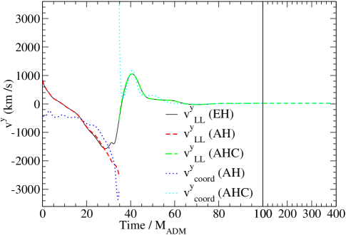
Figure 8: The velocity of the individual and merged black holes. The Landau-Lifshitz velocity $v_{\rm LL}^{y}:=p^{y}_{\rm LL}/p^{t}_{\rm LL}$, where $p^{\mu}_{\rm LL}$ is the Landau-Lifshitz 4-momentum enclosed, is measured on the individual and common apparent horizons (labeled AH and AHC, respectively) and also on the event horizon (labeled EH). For comparison, the coordinate velocities $v^{y}_{\rm coord}$ of the apparent horizons are also shown. The data shown are from the high-resolution evolution $\mbox{N}2.C$.

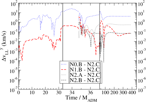
Figure 9: Convergence of $v_{\rm LL}^{y}$ with resolution. Specifically, differences between $v_{\rm LL}^{y}$ at the highest resolution $\mbox{N}2.C$ and at various lower resolutions are shown. Labels of the form $\mbox{N}x.y$ indicate the grid resolution, where the pre-merger resolution is labeled (from coarse to fine) by $x=0,1,2$ and the post-merger resolution is labeled by $y=A,B,C$. The difference between the second-highest and highest resolution is below $0.1\mbox{km/s}$ except near merger, when it grows as large as 1 km/s.

Throughout the pseudospectral evolutions summarized in Sec. III.1.2, we measure the 4-momentum density by explicitly computing the Landau-Lifshitz pseudotensor [Eq. (5)]. Because our evolution variables are essentially the spacetime metric $g_{\mu\nu}$ and its first derivative $g_{\mu\nu,\rho}$, we are able to compute the momentum density without taking any additional numerical derivatives. Besides measuring the momentum density, we also measure the 4-momentum $p^{\mu}_{A}$ [Eq. (9b)] enclosed by i) the apparent horizons, ii) the event horizon, and iii) several spheres of large radius. From the enclosed momentum, we evaluate the effective velocity $v^{j}_{\rm LL}$ [Eq. (10)].

IV.1.1 Apparent horizons

The effective velocities of the apparent horizons are shown in Fig. 8 (dashed curves). To demonstrate convergence, Fig. 9 shows the differences between apparent-horizon effective velocities computed at different resolutions. During the plunge, the difference between the medium and fine resolution is less than 0.1 km/s until shortly before merger, when it reaches a few tenths of a km/s. Shortly after merger, the difference between the highest and medium continuation resolutions between N2.B and N2.C falls from about 1 km/s to about 0.1 km/s.

For comparison, Fig. 8 also shows the apparent horizons’ coordinate velocities (dotted curves); the coordinate and effective velocities agree qualitatively during the plunge and quantitatively during the merger. Also, Fig. 8 shows that the effective velocities of individual apparent horizons and the the event horizon agree well until shortly before merger, when the event horizon’s velocity smoothly transitions to agree with the common apparent horizon’s (cf. Sec. IV.1.2 below).

Because of frame-dragging, during the plunge the individual apparent horizons accelerate in the downward ($-y$) direction, eventually reaching velocities of thousands of km/s. But when the common apparent horizon appears, its velocity is much closer to zero and quickly changes sign, eventually reaching speeds of about 1000 km/s in the $+y$ direction (i.e., in the direction opposite the frame-dragging direction). Then, as the common horizon rings down, the velocity relaxes to a final kick velocity of about 20 km/s in the $+y$ direction.

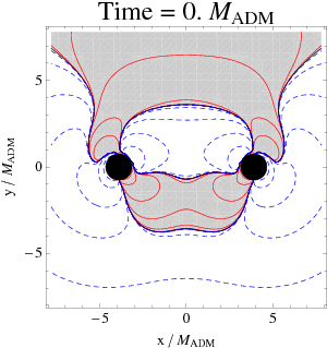
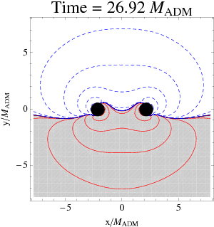
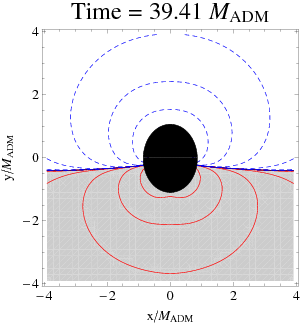
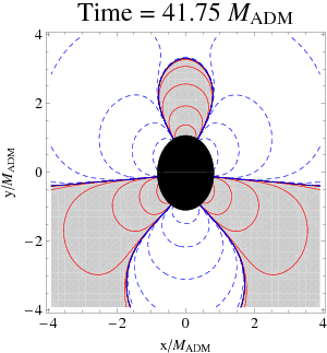
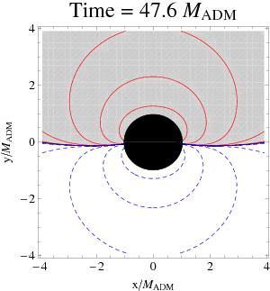
Figure 10: Contour plots of the $y$ (up-down) component of the momentum density, which points along or opposite of the holes’ motion due to frame dragging. Adjacent contours correspond to a factor of 10 difference in the magnitude of the momentum density. Contours of positive $y$ momentum density are shown as solid red lines, while contours of negative $y$ momentum density are shown as dashed blue lines. The region containing positive $y$ momentum density is shaded grey. The regions inside the apparent horizons are shaded black, except for the upper right panel, where the region inside the individual horizons is shaded black, while the common apparent horizon is indicated by a thick black line. The data shown are from the high-resolution evolution $\mbox{N}2.C$.

After merger, why have the horizon velocities suddenly changed from thousands of km/s in the frame-dragging direction to over a thousand km/s in the opposite direction? The answer can be seen in Fig. 10, which plots contours of constant y-momentum density at several times. At $t=0$, the momentum density has an irregular shape, because the initial data is initially not in equilibrium. By time $t=26.92M_{\rm ADM}$, the momentum density has relaxed. When the common apparent horizon forms (at time $t=34.73M_{\rm ADM}$), it encloses not only the momentum of the individual apparent horizons but also the momentum in the gravitational field between the holes.

It turns out that the net momentum outside the individual horizon but inside the common horizon points in the $+y$ direction; as the common horizon expands, it absorbs more and more of this upward momentum. Fig. LABEL:fig:Shape compares the common apparent horizon’s effective velocity to its area and shape; the latter is indicated by the pointwise maximum and minimum of the horizon’s intrinsic scalar curvature. During the first half-period of oscillation (to the left of the leftmost dashed vertical line), the common horizon expands (as seen by its increasing area); as it expands, the upward-pointing linear momentum it encloses causes $v_{\rm LL}^{y}$ to increase. After the first half-period, the horizon shape is maximally oblate (cf. panel B on the right side of of Fig. LABEL:fig:Shape), and $v_{\rm LL}^{y}$ is at its maximum value of about $1000$ km/s.

After another half-period of oscillation, the apparent horizon becomes prolate and encloses enough downward-pointing momentum that $v_{\rm LL}^{\rm eff}$ has decreased to only about $+200$ km/s. After one additional full period, the effective velocity has fallen to nearly zero. As the horizon is ringing down, the momentum density in the surrounding gravitational field also oscillates: the final four panels in Fig. 10 show how the momentum density relaxes to a final state as the horizon relaxes to that of a boosted Schwarzschild black hole.

As the horizon rings down, gravitational waves are emitted, and these waves carry off a small amount of linear momentum. The net radiated momentum is only a small fraction of the momenta of the individual holes at the time of merger: the final effective velocity of the merged hole is about $20$ km/s in the upward-pointing direction, or about 1% of the individual holes’ downward velocity just before merger.

Figure 12: A comparison of various measures of the merged hole’s final velocity. The kick velocity inferred from the gravitational-wave flux (thin dashed lines) and the Landau-Lifshitz effective velocities $v^{y}_{\rm LL}$ (thin solid lines) are measured on spheres of radius $100M_{\rm ADM}$, $120M_{\rm ADM}$, $140M_{\rm ADM}$, and $160M_{\rm ADM}$ The value of the kick velocity at the final time is extrapolated to $r=\infty$ (black cross). The effective velocity measured on the common apparent horizon (thick solid line) and the coordinate velocity (thick dashed line) are also shown. The data shown are from the high-resolution evolution $\mbox{N}2.C$.

Various measures of the final velocity of the merged hole are shown in Fig. 12. The kick velocity $v^{y}_{\rm kick}$, which is inferred from the outgoing gravitational waves, is measured on four coordinate spheres (with radii $R$ of $100M_{\rm ADM}$, $120M_{\rm ADM}$, $140M_{\rm ADM}$, and $160M_{\rm ADM}$); the effective velocity is measured on the same coordinate spheres. We find that the effective velocity $v^{y}_{\rm LL}$ has no significant dependence on the radius of the extraction surface at late times, while $v^{y}_{\rm kick}$ does. The dependence of $v^{y}_{\rm kick}$ on the extraction radius is expected, since our method of extracting $\Psi_{4}$ at finite radius has gauge-dependent contributions that vanish as $R\to\infty$. When $v^{y}_{\rm kick}$ is extrapolated to infinite radius, however, it does agree well (within 0.2 km/s) with $v^{y}_{\rm LL}$. Also, the effective velocity $v^{y}_{\rm LL}$ calculated on the horizon also agrees fairly well (within about 0.5 km/s) with $v^{y}_{\rm LL}$ measured on distant spheres.

IV.1.2 Event horizon

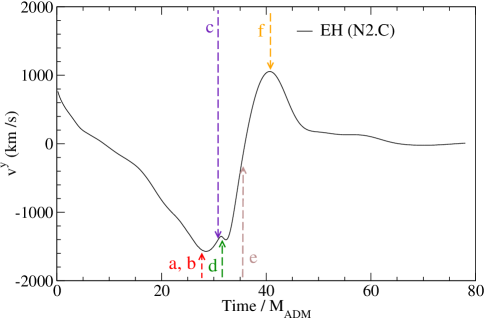
Figure 13: The effective velocity $v_{\rm LL}^{y}$ calculated on the event horizon surface, with the specified snapshots in Fig. 14 of the event horizon surface marked: a,b, $t=27.7M_{\rm ADM}$; c, $t=30.8M_{\rm ADM}$; d, $t=31.6M_{\rm ADM}$; e, $t=35.5M_{\rm ADM}$; f, $t=40.8M_{\rm ADM}.$

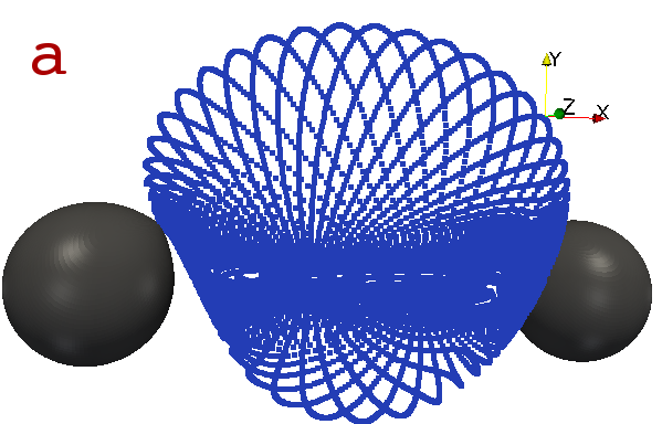
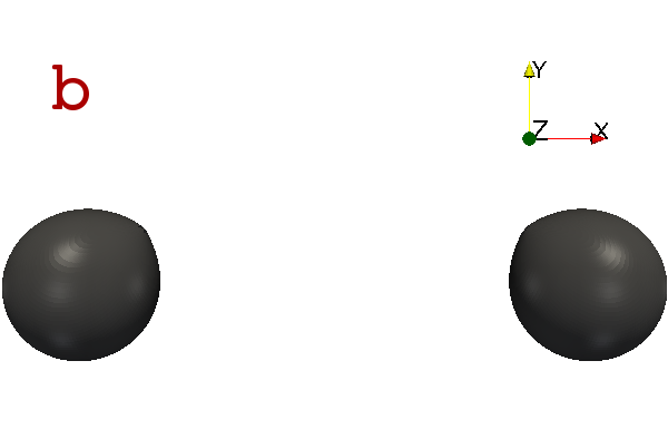
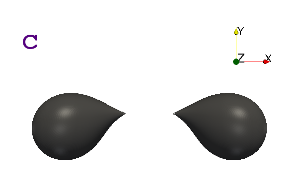
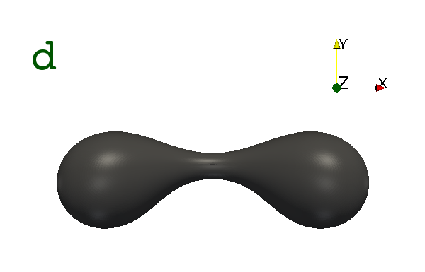
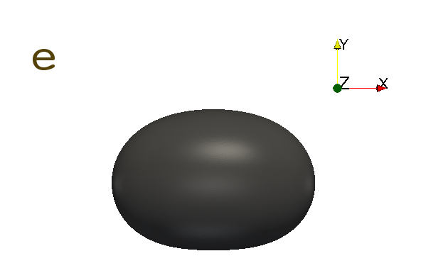
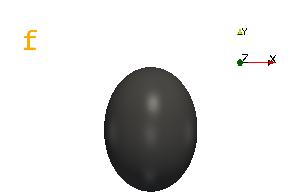
Figure 14: Snapshots of the event horizons at the times indicated in Fig. 13: a,b, $t=27.7M_{\rm ADM}$; c, $t=30.8M_{\rm ADM}$; d, $t=31.6M_{\rm ADM}$; e, $t=35.5M_{\rm ADM}$; f, $t=40.8M_{\rm ADM}.$ All snapshots are looking down the z-axis to the x-y plane, except for shot a, which is slightly skewed (slightly rotated about the y axis) to better see the geodesic structure. In shot a, the future generators of the horizon are visible as small blue dots. Note how the future generators map out a surface that meets the event horizon at the event horizon’s cusps; this is where the future generators join the horizon. The data shown are from the high-resolution evolution $\mbox{N}2.C$.

We would like to compare our quantitative results of the effective velocity $v_{\rm LL}^{y}$ calculated using the event horizon surface (Fig. 13) with qualitative observations of the event horizon’s dynamics (Fig. 14). We find that the greatest variation in both the event horizon geometry and the value of $v_{\rm LL}^{y}$ occurs over a period of about $\Delta t=13M_{\rm ADM}$ from $t=28M_{\rm ADM}$ to $t=41M_{\rm ADM}$. At time $t=27.7M_{\rm ADM}$, the cusps of the event horizon just begin to become noticeable (Figs. 14 a & b). One can see in Fig. 13 that this is the time at which $v_{\rm LL}^{y}$ changes from decreasing to increasing. Shortly after, at $t=31.1M_{\rm ADM}$, the two separate event horizons coalesce into a common event horizon, and the common event horizon rapidly expands to form a convex shape by $t=35.5M_{\rm ADM}$ (Figs. 14 d & e). At this time, we note that $v_{\rm LL}^{y}$ is rapidly increasing (Fig. 13, arrow e); this rapid increase corresponds to the quickly expanding event horizon surface.

We interpret this process as the merging black holes “swallowing” the gravitational field momentum between the holes. The resulting change in $v_{\rm LL}^{y}$ can be divided into two distinct portions: i) one that results from the changing event horizon surface in space, i.e. the field momentum swallowed by the black holes [mathematically, the second term, in Eq. (11)] and ii) a second that results from the change of field momentum at the black holes’ surface, i.e. the field momentum flowing into the black holes [mathematically, the first term, in Eq. (11)]. While this distinction is clearly coordinate dependent, it could, after further investigation, nevertheless provide an intriguing and intuitive picture of the near-zone dynamics of merging black hole binaries.

IV.2 Moving-puncture results and gauge

As summarized in Sec. II, the Landau-Lifshitz formalism that we have applied to our numerical simulations is based on a mapping between the curved spacetime of the simulation and an auxiliary flat spacetime. In the asymptotically-flat region far from the holes, there is a preferred way to construct this mapping. Consequently, when the surface of integration is a sphere approaching infinite radius, Eq. (9b) gives a gauge-invariant measure of the system’s total 4-momentum (see, e.g., Sec. 20.3 of Ref. Misner et al. (1973)). However, when the surface of integration is in the strong-field region of the spacetime (e.g., when the surface is a horizon), the 4-momentum enclosed is gauge dependent. The momentum density, being given by a pseudotensor, is always gauge dependent.

The gauge-dependence of the effective velocity can be investigated at late times—when the spacetime has relaxed to its final, stationary configuration—by comparing the velocity obtained on the horizon with gauge-invariant measures of the kick velocity (Fig. 12). At the final time in our pseudospectral simulation, the effective velocities of the apparent and event horizons agree within tenths of a km/s with the (extrapolated) kick velocity inferred from the gravitational-wave flux; at late times, the horizon effective velocities also agree with the effective velocity measured on coordinate spheres of large radius. At least at late times, then, the effective velocity $v^{y}_{\rm LL}$ is not significantly affected by our choice of gauge.

But how strong is the influence of gauge on our results in the highly-dynamical portion of the evolution, when we have no gauge-invariant measure of momentum or velocity? To investigate this, we have evolved initial data that are physically similar using two manifestly different gauge conditions: i) the generalized-harmonic condition used in our spectral evolutions, and ii) the “1+log” slicing and “Gamma-driver” shift conditions used in our moving-puncture evolutions.

Figs. 15 and 16 display the velocity obtained from the horizon integral of the components of the Landau-Lifshitz tensor in the moving-puncture evolutions described in Sec. III.2.2. The most remarkable feature in these plots is a large temporary acceleration of the black holes in the frame-dragging direction. The magnitude of the velocity reaches about $4500~{}{\rm km/s}$, which is of the order of the superkicks first reported in Refs. Gonzalez et al. (2007b); Campanelli et al. (2007a).

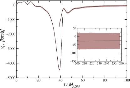
Figure 15: Velocity perpendicular to the line of sight associated with the horizon integrals of the the Landau-Lifshitz tensor obtained for model P1. The shaded area represents the numerical uncertainty. During the pre-merger phase, the velocities of both holes are identical.

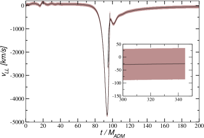
Figure 16: Same as Fig. 15 for model P2 of Table 1.

In contrast to those inspiraling configurations, however, the black hole motion reverses during the merger and settles down to a small value of $-30\pm 50~{}{\rm km/s}$.

In order to examine to what extent this behavior is dependent on specific properties of the puncture evolution (such as the particular form of the spurious radiation, which differs in our spectral and puncture evolutions), we have performed the following additional simulations. First, we have changed the gauge parameter $\eta$ in Eq. (51) to $0.75$ and $1.25$. We do not observe a significant change in the behavior of the effective velocity for this modification.

Second, in order to gain further insight into the dependence of the effective velocity on the initial separation of the black holes, we have increased the initial separation of the holes to allow for a longer pre-merger interaction phase; We study the evolution of the second model P2 in Table 1. This simulation has been performed with the Lean code as summarized in Sec. III.2.1 using a resolution $h_{\rm c}=M_{\rm ADM}/49.8$. The resulting velocity is shown in Fig. 16 and represents numerical uncertainties as gray shading. The remarkable similarity between the figure and its counterpart Fig. 15 for model P1 demonstrates that the numerical results are essentially independent of the initial separation.

Comparing Figs. 8 and 15, the qualitative behavior of the apparent horizons’ effective velocities agrees. In both the spectral and puncture simulations:

1. during the plunge, the individual apparent horizons accelerate to speeds larger than 1000 km/s in the frame dragging direction,

2. when the common horizon forms, its velocity is much smaller in magnitude, because the common horizon has enclosed momentum pointing opposite the frame-dragging direction, and

3. the velocity relaxes to a value of only tens of km/s that (within numerical uncertainty) agrees with the kick velocity measured using the gravitational-wave flux.

These results are particularly encouraging because two popular gauge choices used in the NR community give remarkable overall agreement. While this qualitative agreement certainly does not constitute a proof of a gauge independence of our findings, we feel encouraged in our hope that different types of observers might agree on their overall perception of the local black-hole dynamics during the collision. Most importantly from a practical point of view, it appears possible that such local descriptions can be derived from the current generation of BBH codes without the different numerical relativity groups having to agree upon one and the same gauge choice for comparing their momentum densities and effective velocities. Future investigations using a wider class of coordinate conditions should further clarify the significance of gauge choices in this context.

IV.3 Comparison with post-Newtonian predictions

In this section we compare our results to post-Newtonian predictions. For each comparison, first the S1 data set (Table 1) is presented along with post-Newtonian predictions of a corresponding initial configuration, then the H1 data set (Table 1) is presented along with its post-Newtonian predictions. The post-Newtonian trajectories for spinning point particles were generated by evolving the post-Newtonian equations of motion Faye et al. (2006); Tagoshi et al. (2001). The difference between the two data sets are: i) set H1 begins with a larger initial separation than set S1, and ii) set H1 is evolved in a nearly harmonic gauge. Comparing evolutions of data sets S1 and H1 illustrates how these two effects improve the comparisons one can make with post-Newtonian predictions.

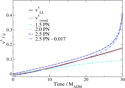
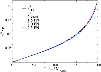
Figure 17: A comparison of numerical and post-Newtonian longitudinal velocities (i.e., $v^{x}/c$) versus time. The predicted coordinate velocities at several post-Newtonian orders are shown as broken curves. Left: A comparison of S1 numerical data and post-Newtonian predictions. The numerical and post-Newtonian curves agree qualitatively. When the 2.5 PN curve is offset by a certain amount, it agrees quantitatively with the coordinate velocity $v^{x}_{\rm coord}$ and the effective velocity $v^{x}_{\rm LL}$. Right: A comparison of H1 numerical data and PN predictions. The effective velocity $v^{x}_{\rm LL}$ (thick black line) closely tracks the coordinate velocity $v^{x}_{\rm coord}$; both numerical curves also agree well with the 2.0 PN and 2.5 PN curves.

The left panels of Figs. 17–19 show the comparison between the highest-resolution evolution ($\mbox{N}2.C$) of initial data set S1 and several orders of post-Newtonian predictions. The right panels of Figs. 17–19 show analogous comparisons with an evolution of initial data set H1.

Figure 17 shows that the bulk, longitudinal motions (i.e., motion in the $x$ direction) agree both qualitatively and quantitatively with post-Newtonian predictions through most of the plunge (i.e., a few $M_{\rm ADM}$ before the formation of the common apparent horizon) for both data sets. In the left panel of Fig. 17, we have added another 2.5 PN curve that is offset vertically such that the 2.5 PN coordinate velocity agrees exactly with the numerical effective velocity at $t\approx 18.34M_{\rm ADM}$; this is done in order to account for the period of initial relaxation in the S1 data set. Quantitative agreement is then found between 2.5 PN predictions and both the effective and coordinate velocities from $t\approx 5M_{\rm ADM}$ through $t\approx 20M_{\rm ADM}$. The right panel of Fig. 17, which has less of an initial relaxation due to the increased separation, shows excellent agreement between both the effective and coordinate velocities and the 2.0 PN and 2.5 PN predictions.

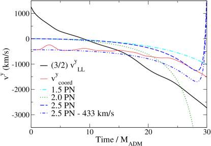
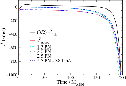
Figure 18: A comparison of numerical and post-Newtonian transverse velocities (i.e., $v^{y}$ in km/s) versus time. The left panel shows numerical results from simulation S1, while the right panel shows numerical results from simulation H1. The predicted coordinate velocity at several post-Newtonian orders are shown as broken curves. The effective velocity is shown in black; it has been rescaled by a factor of $3/2$ in order to aid comparison with the post-Newtonian point-particle velocities, as discussed in the text.

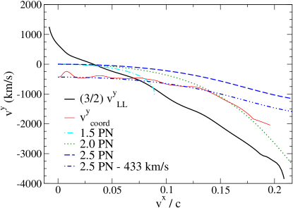
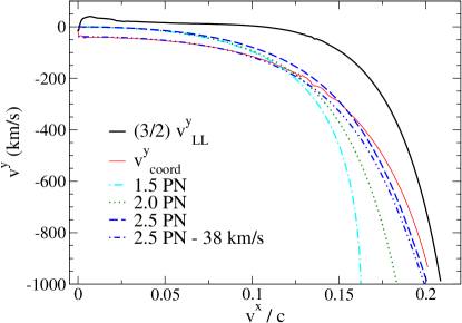
Figure 19: A comparison of numerical and post-Newtonian velocities. In the figure, $v^{y}$ in km/s is plotted against $v^{x}/c$. The effective velocity $v^{y}_{\rm LL}$ of the highest-resolution ($\mbox{N}2.C$) evolution of initial data S1 (Table 1) on the left and of the evolution of initial data H1 (Table 1) on the right are shown as a thick black line. The predicted coordinate velocity at several post-Newtonian orders are shown as broken curves. The transverse effective velocities only agree qualitatively with post-Newtonian predictions; however, the coordinate velocity agrees very well with post-Newtonian predictions. In the left panel, the coordinate velocity has been artificially truncated shortly before merger because at that point we do not have a good measure of the coordinate velocity. The effective velocity has been rescaled by a factor of $3/2$ to aid comparison with the post-Newtonian point-particle velocities, as discussed in the text.

For the minor (yet more interesting) transverse motion (i.e., the motion along the $y$ direction), we find only qualitative agreement between the numerical data and post-Newtonian predictions—spin-orbit coupling [more specifically, frame-dragging plus spin-curvature coupling, see Eq. (5.11) of paper I and discussions thereafter] cause the holes to move in the $-y$ direction during the plunge, reaching speeds of order 1000 km/s before the holes merge. The post-Newtonian expansion scheme we adopt (paper I and Refs. Faye et al. (2006); Tagoshi et al. (2001)) uses a harmonic gauge, and a physical spin supplementary condition (SSC) of $S^{\alpha\beta}u_{\beta}=0$, where $S^{\alpha\beta}$ is the spin angular momentum tensor of the black hole and $u^{\beta}$ its four velocity (see e.g., Sec. II B of paper I).

In this scheme, for the equal-mass–opposite-spin configuration, up to the leading 1.5 PN order, the coordinate $y$ velocity of the point particle representing each hole is equal to $3/2$ the hole’s effective velocity, $v^{y}_{\rm LL}$, evaluated through a surface integral of the post-Newtonian expression for the super potential [cf. Eq. (9b)]. Therefore, in Figs. 18–19 we rescale the effective velocity $p^{y}_{\rm LL}$ by this factor of 3/2, which arises from our particular choice of SSC and from field momentum distribution in the vicinity of the holes (see Secs. II B and II C, and Table I of paper I for details).

In Figs. 18 and 19, we compare the post-Newtonian point-particle $y$ velocity with the numerical coordinate $y$ velocity and $3/2$ of the numerical effective $y$ velocity $v^{y}_{\rm LL}$. For the comparison to the S1 data set, we find qualitative agreement with both the effective and coordinate velocities and the post-Newtonian predictions. We think this agreement is not better because of the large initial relaxations present in the S1 data set related to small initial separation. However, in the H1 comparison, we find excellent agreement between the coordinate velocity and the 2.5 PN prediction but only qualitative agreement between the effective velocity and post-Newtonian predictions. In these figures, offsets of $-$433 km/s (for S1 data) and $-$38 km/s (for H1 data) have been used to make 2.5 PN coordinate velocity agree better with numerical results. Such offsets can be motivated as follows. Our numerical initial data were chosen such that the initial total momentum of the entire spacetime vanishes. This, in our post-Newtonian scheme, corresponds to nonvanishing initial $y$ velocities of (see Table I of paper I)

$$v^{y}_{\rm coord}=\frac{\chi}{4(r_{0}/M_{\rm ADM})^{2}}\,,$$ (16)

where $\chi$ is the spin parameter of each hole, and $r_{0}$ their initial separation. This corresponds to $-616$ km/s for the S1 data, and $-42$ km/s for H1 data. Again, the agreement is qualitative for S1 data, and quantitative for H1 data.

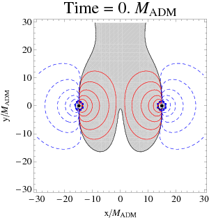
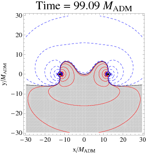
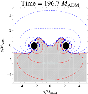
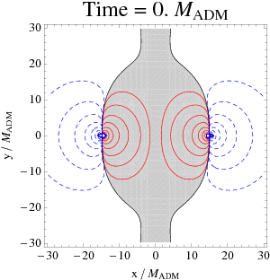
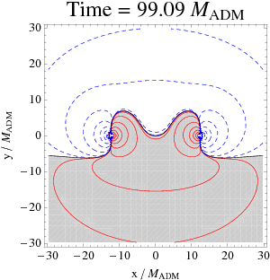
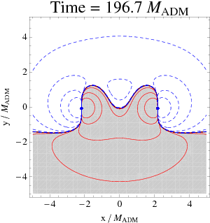
Figure 20: Comparison of numerical (top row) and post-Newtonian (bottom row) $y$ momentum density. The numerical data comes from the harmonic evolution H1 described in Appendix D. The 1.5 PN momentum density is computed from Eqs. (A2a)–(A2c) in paper I using the numerical hole trajectories. As in Fig. 10, contours represent powers of $10$ in $y$ momentum density. The positive $y$ momentum density contours are shown in red, negative in blue. The region of positive $y$ momentum density is shaded grey. In the numerical plots the apparent horizons are shown in black.

One final comparison we make between the H1 data set and post-Newtonian predictions is the near-field momentum density, shown in Fig. 20. The numerical data comes from the harmonic evolution H1, while the 1.5 PN momentum density is computed from Eqs. (A2a)-(A2c) in paper I using the numerical hole trajectories. The left panels, comparing the initial data to the predicted post-Newtonian momentum density, show differences which are presumably due to differences in the post-Newtonian and numerical initial data, such as the numerical initial data being out of equilibrium. The center panels show the momentum densities agree very well once enough time has elapsed for the spacetime to relax and for the spurious radiation to be emitted but before the holes have fallen too close together. The right panels make a final comparison just before the holes get close enough to merge and shows differences appearing between the numerical data and the post-Newtonian predictions very near the holes—which could be an indication of the breakdown of the post-Newtonian approximation.

These comparisons with post-Newtonian predictions have yielded several interesting results. The primary result of these comparisons is the surprisingly good agreement found between post-Newtonian predictions and the coordinate velocities, especially from the harmonic gauge evolution. Also, the longitudinal effective and coordinate velocities track each other; consequently, the longitudinal effective velocity agrees with post-Newtonian predictions. The transverse effective velocities agree qualitatively with the post-Newtonian predictions in the sense that they both indicate that the holes accelerate in the expected frame-dragging direction to speeds of order 1000 km/s. Finally, we have also found the qualitative agreement between harmonic gauge numerical data and post-Newtonian extends to the near-zone momentum density after the initial data relaxes but before the holes have fallen too close together.

V Conclusion

With the goal of building up greater physical intuition, we have used the Landau-Lifshitz momentum-flow formalism to explore the nonlinear dynamics of fully relativistic simulations of a head-on BBH plunge, merger, and ringdown. We have defined and computed an effective velocity of the black holes in terms of the momentum and mass-energy enclosed by their horizons, and we have interpreted the holes’ transverse motion—which reaches speeds of order 1000 km/s—as a result of momentum flow between the holes and the gravitational field of the surrounding spacetime. We have found that the merged hole’s final effective velocity—about 20 km/s—agrees with the recoil velocity implied by the momentum carried off by the emitted gravitational waves.

Our measures of linear momentum and effective velocity are gauge dependent. Nonetheless, after comparing simulations of comparable initial data in generalized-harmonic and moving-puncture gauges, we have observed remarkably weak gauge dependence for the generalized-harmonic and moving-puncture evolutions discussed in this paper. Additionally, we have found surprisingly good agreement between the holes’ effective and coordinate velocities, and at late times, the holes’ final effective velocities and gauge-invariant measures of the kick velocity agree.

These results motivate future explorations of momentum flow in fully-relativistic numerical simulations that are more astrophysically realistic. We are particularly eager to investigate simulations of superkick BBH mergers (the inspiral of a superkick configuration was considered using the post-Newtonian approximation in paper I). Other future work includes studies of the linear and angular momentum flow in inspiraling (rather than head-on) mergers as well as mergers with larger spins.

Appendix A Superposed-Kerr-Schild (SKS) initial data

The initial data for the pseudospectral simulations presented in this paper was constructed using the methods described in Ref. Lovelace et al. (2008). In this appendix, we describe in more detail these initial data (which we summarize in Sec. III.1.1).

The usual 3+1 decomposition splits the spacetime metric $g_{\mu\nu}$ into a spatial metric $\gamma_{ij}$, lapse $\alpha$, and shift $\beta^{i}$, i.e.

$$ds^{2} = g_{\mu\nu}dx^{\mu}dx^{\nu}=-\alpha^{2}dt^{2}$$ (17)

$$+ \gamma_{ij}(dx^{i}+\beta^{i}dt)(dx^{j}+\beta^{j}dt).$$

On the initial spatial slice (at time $t=0$), the initial data must specify the spatial metric $\gamma_{ij}$ and the extrinsic curvature $K_{ij}$, which is related to the time derivative of the spatial metric by

$$\partial_{t}\gamma_{ij}=-2\alpha K_{ij}+2\nabla_{(i}\beta_{j)}.$$ (18)

We use the quasiequilibrium formalism Cook (2002); Cook and Pfeiffer (2004); Caudill et al. (2006); Gourgoulhon et al. (2002); Grandclément et al. (2002), in which $\gamma_{ij}$ and $K_{ij}$ are expanded as

$$\gamma_{ij}=\psi^{4}\tilde{\gamma}_{ij},$$

$$K_{ij}=A_{ij}+\frac{1}{3}\gamma_{ij}K.$$ (19)

The conformal metric $\tilde{\gamma}_{ij}$, the trace of the extrinsic curvature $K$, and their time derivatives can be chosen freely. We adopt the quasiequilibrium choices

$$\tilde{u}_{ij}:=\partial_{t}\tilde{\gamma}_{ij}=0,$$

$$\partial_{t}K=0.$$ (20)

The remaining free data are based on a weighted superposition of two boosted, spinning Kerr-Schild black holes (Eqs. (45)–(46) of Ref. Lovelace et al. (2008)):

$$\tilde{\gamma}_{ij} := f_{ij}+\sum_{a=1}^{2}e^{-r_{a}^{2}/w_{a}^{2}}\left(\gamma_{ij}^{a}-f_{ij}\right),$$ (21)

$$K := \sum_{a=1}^{2}e^{-r_{a}^{2}/w_{a}^{2}}K_{a}..$$ (22)

Here $f_{ij}$ is the metric of flat space, $r_{a}$ is the Euclidean distance from the center of the apparent horizon of hole $a$, and $\gamma_{ij}^{a}$ and $K_{a}$ are the spatial metric and mean curvature of a boosted (with velocity $\tilde{v}^{i}$), spinning (with spin $\tilde{S}/\tilde{M}^{2}$) Kerr-Schild black hole centered at the initial position of hole $a$. In this paper we choose $\tilde{v}^{i}=0$ (since we seek data describing holes falling head-on from rest), $\tilde{M}=0.39M_{\rm ADM}$, and $\tilde{S}/\tilde{M}^{2}=0.5$. The Gaussian weighting parameter is chosen to be $w_{a}=d/3$, where $d$ is the initial coordinate separation between the two holes; note that this choice causes the conformal metric to be flat everywhere except near each hole. The holes are located at coordinates $(x,y,z)=(x_{0}\equiv\pm d/2,0,0)$.

These free data are then inserted into the extended conformal thin sandwich (XCTS) equations (e.g., Eqs. (13)–(15) of Ref. Cook and Pfeiffer (2004)), which are then solved for the conformal factor $\psi$, the lapse $\alpha$, and the shift $\beta^{i}$:

$${\tilde{\nabla}}^{2}\psi-\frac{1}{8}\tilde{R}\psi - \frac{1}{12}K^{2}\psi^{5}+\frac{1}{8}\psi^{-7}\tilde{A}^{ij}\tilde{A}_{ij}=0,$$

$${\tilde{\nabla}}\!_{j}\Big{(}\frac{\psi^{7}}{2(\alpha\psi)}(\tilde{\mathbb{L}}{\beta})^{ij}\Big{)} - \frac{2}{3}\psi^{6}{\tilde{\nabla}}^{i}K-{\tilde{\nabla}}\!_{j}\Big{(}\frac{\psi^{7}}{2(\alpha\psi)}\tilde{u}^{ij}\Big{)}=0,$$

$${\tilde{\nabla}}^{2}(\alpha\psi) - (\alpha\psi)\bigg{[}\frac{\tilde{R}}{8}\!+\!\frac{5}{12}K^{2}\psi^{4}\!+\!\frac{7}{8}\psi^{-8}\tilde{A}^{ij}\tilde{A}_{ij}\bigg{]}$$ (23)

$$= -\psi^{5}(\partial_{t}K-\beta^{k}\partial_{k}K),$$

where the Ricci scalar curvature of the conformal metric $\tilde{\gamma}_{ij}$ is $\tilde{R}$, the longitudinal derivative $\tilde{\mathbb{L}}$ is defined as

$$(\tilde{\mathbb{L}}V)_{ij}:=\tilde{\nabla}_{i}V_{j}+\tilde{\nabla}_{j}V_{i}-\frac{2}{3}\tilde{\gamma}_{ij}\tilde{\nabla}_{k}V^{k},$$ (24)

and the trace-free part of the extrinsic curvature $A^{ij}$ satisfies

$$\tilde{A}^{ij}=\psi^{10}A^{ij}=\frac{\psi^{7}}{2(\alpha\psi)}\left[(\tilde{\mathbb{L}}\beta)^{ij}-\tilde{u}^{ij}\right].$$

The XCTS equations are solved using a spectral elliptic solver Pfeiffer et al. (2003) on a computational domain with i) a very large outer boundary (which is chosen to be a coordinate sphere with radius $10^{9}\tilde{M}$), and ii) with the region inside the holes’ apparent horizons excised. The excision surfaces $\mathcal{S}$ are surfaces of constant Kerr radius $r_{\rm Kerr}$, where

$$\frac{x^{2}+y^{2}}{r_{\rm Kerr}^{2}+\tilde{S_{a}}^{2}/\tilde{M_{a}}^{2}}+\frac{z^{2}}{r_{\rm Kerr}^{2}}=1.$$ (25)

The excision surfaces are the apparent horizons of the holes; this is enforced by the following boundary condition: (Eq. (48) of Ref. Cook and Pfeiffer (2004)):

$$\tilde{s}^{k}\partial_{k}\psi = -\frac{\psi^{-3}}{8\tilde{\alpha}}\tilde{s}^{i}\tilde{s}^{j}\left[(\tilde{\mathbb{L}}{\beta})_{ij}-\tilde{u}_{ij}\right]$$ (26)

$$-\frac{\psi}{4}\,\tilde{h}^{ij}{\tilde{\nabla}}\!_{i}\tilde{s}_{j}+\frac{1}{6}K\psi^{3}\mbox{ on }\mathcal{S}.$$

Here $\tilde{s}^{i}:=\psi^{2}s^{i}$, $s^{i}$ is a unit vector normal to the excision surface $\mathcal{S}$, and $\tilde{h}_{ij}:=\tilde{\gamma}_{ij}-\tilde{s}_{i}\tilde{s}_{j}$ is the induced metric on the excision surface.

On the apparent horizon, the lapse satisfies the boundary condition

$$\alpha\psi=1+\sum_{a=1}^{2}e^{-r_{a}^{2}/w_{a}^{2}}(\alpha_{a}-1)\mbox{ on }\mathcal{S},$$ (27)

where $\alpha_{a}$ is the lapse of the Kerr-Schild metric corresponding to hole $a$. The shift satisfies

$$\beta^{i}=\alpha s^{i}-\Omega_{r}\xi^{i}\mbox{ on }\mathcal{S}.$$ (28)

The first term in Eq. (28) implies that the holes are initially at rest, and the second term determines the spin of the hole; to make the spin point in the $\pm z$ direction with magnitude $S/M_{\rm Chr}^{2}=0.5$ (measured using the method described in Appendix A of Ref. Lovelace et al. (2008)), we choose $M_{\rm ADM}\Omega_{r}=\mp 0.244146$ and $\xi^{i}=\partial_{\phi}$, where $\partial_{\phi}$ is the rotation vector on the apparent horizon corresponding to rotation about the $+z$ axis.

On the outer boundary $\mathcal{B}$, the spacetime metric is flat:

$$\psi = 1\mbox{ on }\mathcal{B},$$ (29)

$$\alpha\psi = 1\mbox{ on }\mathcal{B}.$$ (30)

Because the holes are initially at rest in the coordinates, they can be given orbital, radial, and translational motion by rotation, expansion, and translation of the shift on the outer boundary, i.e.

$$\beta^{i}=\left(\mathbf{\Omega}_{0}\times r\right)^{i}+\dot{a}_{0}r^{i}+V_{0}^{i},\mbox{ on }\mathcal{B}.$$ (31)

We choose $\dot{a}_{0}=0$ and $\Omega$ = 0. To make the total momentum of the initial data vanish, we choose $V^{i}=-0.001444$.

Our initial data are constructed [Eq. (28)] in a frame comoving with the black holes. Thus, an asymptotic rotation, expansion, and translation in the comoving shift $\beta^{i}$ cause the holes to initially have radial, angular, or translational velocity in the inertial frame. Note that the initial data are evolved in inertial, not comoving, coordinates, so that the shift during the evolution is different from the comoving shift $\beta^{i}$ obtained from the XCTS equations: the former asymptotically approaches zero, not a constant vector $V_{0}^{i}$.

Appendix B Numerical methods for evolutions

B.1 Pseudospectral evolutions

We evolve the initial data summarized in Sec. III.1.1 using the Caltech-Cornell pseudospectral code SpEC. This code and the methods it employs are described in detail in Refs. Scheel et al. (2006); Boyle et al. (2007); Scheel et al. (2009). Some of these methods have been simplified for the head-on problem discussed here, and others have been modified to account for a nonzero center-of-mass velocity, so we will describe them here.

We evolve a first-order representation Lindblom et al. (2006) of the generalized harmonic system Friedrich (1985); Garfinkle (2002); Pretorius (2005b). We handle the singularities by excising the black hole interiors from the computational domain. Our outer boundary conditions Lindblom et al. (2006); Rinne (2006); Rinne et al. (2007) are designed to prevent the influx of unphysical constraint violations Stewart (1998); Friedrich and Nagy (1999); Bardeen and Buchman (2002); Szilágyi et al. (2002); Calabrese et al. (2003); Szilágyi and Winicour (2003); Kidder et al. (2005) and undesired incoming gravitational radiation Buchman and Sarbach (2006, 2007) while allowing outgoing gravitational radiation to pass freely through the boundary.

We employ the dual-frame method described in Ref. Scheel et al. (2006): we solve the equations in an “inertial frame” that is asymptotically Minkowski, but our domain decomposition is fixed in a “comoving frame” that is allowed to shrink, translate and distort relative to the inertial frame. The positions of the centers of the black holes are fixed in the comoving frame; we account for the motion of the holes by dynamically adjusting the coordinate mapping between the two frames. Note that the comoving frame is referenced only internally in the code as a means of treating moving holes with a fixed domain. Therefore all coordinate quantities (e.g. black hole trajectories) mentioned in this paper are inertial-frame values unless explicitly stated otherwise.

The mapping from comoving to inertial coordinates is changed several times during the run. During the plunge phase, we denote the mapping by ${\cal M}_{\rm p}(x^{i},x^{\prime i})$, where primed coordinates denote the comoving frame and unprimed coordinates denote the inertial frame. Explicitly, ${\cal M}_{\rm p}(x^{i},x^{\prime i})$ is the mapping

$$x = F(r^{\prime},t)\sin\theta^{\prime}\cos\phi^{\prime},$$ (32)

$$y = F(r^{\prime},t)\sin\theta^{\prime}\sin\phi^{\prime}+e^{-r^{\prime 2}/r^{\prime 2}_{\rm T}}Y(t),$$ (33)

$$z = F(r^{\prime},t)\cos\theta^{\prime}\cos\phi^{\prime},$$ (34)

where

$$F(r^{\prime},t) := r^{\prime}\left[a(t)+\left(1-a(t)\right)\frac{r^{\prime 2}}{R_{0}^{\prime 2}}\right].$$ (35)

Here $a(t)$ and $Y(t)$ are functions of time, $(r^{\prime},\theta^{\prime},\phi^{\prime})$ are spherical polar coordinates in the comoving frame centered at the origin, and $R_{0}^{\prime}$ and $r^{\prime}_{\rm T}$ are constants. For the choice $R_{0}^{\prime}=\infty$ and $r^{\prime}_{\rm T}=\infty$, the mapping is simply an overall contraction by $a(t)\leq 1$ plus a translation $Y(t)$ in the $y$ direction. Choosing $R_{0}^{\prime}$ equal to the outer boundary radius $R^{\prime}_{\rm max}$ and choosing $r^{\prime}_{\rm T}\sim R^{\prime}_{\rm max}/6$ causes the map to approach the identity near the outer boundary; this prevents the outer boundary from falling close to the strong-field region during merger, and makes it easier to keep the outer boundary motion smooth through the merger/ringdown transition. The functions $a(t)$ and $Y(t)$ are determined by dynamical control systems as described in Ref. Scheel et al. (2006). These control systems adjust $a(t)$ and $Y(t)$ so that the centers of the apparent horizons remain stationary in the comoving frame. For the evolutions presented here, we use $R_{0}^{\prime}=532.2M_{\rm ADM}=1.1R^{\prime}_{\rm max}$ and $r^{\prime}_{\rm T}=31.21M_{\rm ADM}=4d_{o}$, where $d_{o}$ is the initial separation of the holes.

The gauge freedom in the generalized harmonic system is fixed via a freely specifiable gauge source function $H_{a}$ that satisfies the constraint

$$0=\mathcal{C}_{a}:=\Gamma_{ab}{}^{b}+H_{a},$$ (36)

where $\Gamma^{a}{}_{bc}$ are the spacetime Christoffel symbols. To choose this gauge source function, we define a new quantity $\tilde{H}_{a}$ that transforms like a tensor and agrees with $H_{a}$ in inertial coordinates (i.e. $\tilde{H}_{a}=H_{a}$). Then we choose $\tilde{H}_{a}$ so that the constraint (36) is satisfied initially, and we demand that $\tilde{H}_{a^{\prime}}$ is constant in the moving frame.

Shortly before merger (at time $t_{1}=31.1M_{\rm ADM}$), we make two modifications to our algorithm to reduce numerical errors and gauge dynamics during merger. First, we begin controlling the size of the individual apparent horizons so that they remain constant in the comoving frame, and therefore they remain close to their respective excision boundaries. This is accomplished by changing the map between comoving and inertial coordinates as follows. We define the map ${\cal M}_{\rm AH_{1}}(\tilde{x}^{i},x^{\prime i})$ for black hole 1 as

$$\tilde{x} = x^{\prime}_{\rm AH_{1}}+\bar{r}\sin\theta^{\prime}\cos\phi^{\prime},$$ (37)

$$\tilde{y} = y^{\prime}_{\rm AH_{1}}+\bar{r}\sin\theta^{\prime}\sin\phi^{\prime},$$ (38)

$$\tilde{z} = z^{\prime}_{\rm AH_{1}}+\bar{r}\cos\theta^{\prime},$$ (39)

$$\bar{r} := r^{\prime}-e^{-(r^{\prime}-r^{\prime}_{0})^{3}/\sigma_{1}^{3}}\lambda_{1}(t),$$ (40)

where $(r^{\prime},\theta^{\prime},\phi^{\prime})$ are spherical polar coordinates centered at the (fixed) comoving-coordinate location of black hole 1, which we denote as $(x^{\prime}_{\rm AH_{1}},y^{\prime}_{\rm AH_{1}},z^{\prime}_{\rm AH_{1}})$. The constant $R^{\prime}_{\rm AH_{1}}$ is the desired average radius (in comoving coordinates) of black hole 1. Similarly, we define the map ${\cal M}_{\rm AH_{2}}(\tilde{x}^{i},x^{\prime i})$ for black hole 2. Then the full map from the comoving coordinates $x^{\prime i}$ to the inertial coordinates $x^{i}$ is given by

$${\cal M}_{\rm m}(x^{i},x^{\prime i}):={\cal M}_{\rm p}(x^{i},\bar{x}^{i}){\cal M}_{\rm AH_{2}}(\bar{x}^{i},\tilde{x}^{i}){\cal M}_{\rm AH_{1}}(\tilde{x}^{i},x^{\prime i}).$$ (41)

The constants $\sigma_{1}$, $\sigma_{2}$, and $r^{\prime}_{0}$ are chosen to be $0.780M_{\rm ADM}$, $0.780M_{\rm ADM}$, and $1.01M_{\rm ADM}$, respectively. The functions $\lambda_{1}(t)$ and $\lambda_{2}(t)$ are determined by dynamical control systems that drive the comoving-coordinate radius of the apparent horizons towards their desired values $R^{\prime}_{\rm AH_{1}}=R^{\prime}_{\rm AH_{2}}=1.56M_{\rm ADM}$ Note that in comoving coordinates, the shape of the horizons is not necessarily spherical; only the average radius of the horizons is controlled.

The second change we make at time $t_{1}=31.1M_{\rm ADM}$ is to smoothly roll gauge source function $H_{a}$ to zero by adjusting $\tilde{H}_{a^{\prime}}(t)$ according to

$$\tilde{H}_{a^{\prime}}(t)=\tilde{H}_{a^{\prime}}(t_{1})e^{-(t-t_{1})^{2}/\tau^{2}},$$ (42)

where $\tau=0.5853M_{\rm ADM}.$ This choice makes it easier for us to continue the evolution after the common horizon has formed, and it also reduces gauge dynamics that otherwise cause oscillations in the observed Landau-Lifshitz velocity $v^{y}_{\rm LL}$ during the ringdown.

When the two black holes are sufficiently close to one another, a new apparent horizon suddenly appears, encompassing both black holes. At time $t_{m}=34.73M_{\rm ADM}$ (which is shortly after the common horizon forms), we interpolate all variables onto a new computational domain that contains only a single excised region, and we choose a new comoving coordinate system so that the merged (distorted, pulsating) apparent horizon remains spherical in the new comoving frame. This is accomplished in the same way as described in Section II.D. of Scheel et al. (2009), except that here the map from the new comoving coordinates to the inertial coordinates contains an additional translation in the $y$ direction that handles the nonzero velocity of the merged black hole. In Scheel et al. (2009) a third change, namely a change of gauge, was necessary to continue the simulation after merger. But in the simulations discussed here, Eq. (42) has caused $H_{a}$ to fall to zero by the time of merger, and we find it suffices to simply allow $H_{a}$ to remain zero after merger.

For completeness, we now explicitly describe the map from the new comoving coordinates $x^{\prime\prime i}$ to the inertial coordinates $x^{i}$. This map is given by

$$x = r\sin\theta^{\prime\prime}\cos\phi^{\prime\prime},$$ (43)

$$y = r\sin\theta^{\prime\prime}\sin\phi^{\prime\prime}+e^{-r^{\prime\prime 2}/r^{\prime\prime 2}_{\rm T}}Y(t),$$ (44)

$$z = r\cos\theta^{\prime\prime},$$ (45)

$$r = \tilde{r}\biggr{[}1+\sin^{2}(\pi\tilde{r}/2R^{\prime\prime}_{\rm max})$$ (46)

$$\left.\times\left(A(t)\frac{R^{\prime}_{\rm max}}{R_{\rm max}^{\prime\prime}}+(1-A(t))\frac{R_{\rm max}^{\prime 3}}{R_{\rm max}^{\prime\prime}R_{0}^{\prime 2}}-1\right)\right],$$

$$\tilde{r} = r^{\prime\prime}-q(r^{\prime\prime})\sum_{\ell=0}^{\ell_{\rm max}}\sum_{m=-\ell}^{\ell}\lambda_{\ell m}(t)Y_{\ell m}(\theta^{\prime\prime},\phi^{\prime\prime}),$$ (47)

$(r^{\prime\prime},\theta^{\prime\prime},\phi^{\prime\prime})$ are spherical polar coordinates in the new comoving coordinate system, $R^{\prime\prime}_{\rm max}$ is the value of $r^{\prime\prime}$ at the outer boundary, and $r^{\prime\prime}_{\rm T}$ is a constant chosen to be $31.21M_{\rm ADM}$. The function $q(r^{\prime\prime})$ is given by

$$q(r^{\prime\prime})=e^{-(r^{\prime\prime}-R^{\prime\prime}_{\rm AH})^{3}/\sigma_{q}^{3}},$$ (48)

where $R^{\prime\prime}_{\rm AH}$ is the desired radius of the common apparent horizon in comoving coordinates. The function $A(t)$ is

$$A(t)=A_{0}+(A_{1}+A_{2}(t-t_{m}))e^{-(t-t_{m})/\tau_{A}},$$ (49)

where the constants $A_{0}$, $A_{1}$, and $A_{2}$ are chosen so that $A(t)$ matches smoothly onto $a(t)$ from Eq. (35): $A(t_{m})=a(t_{m})$, $\dot{A}(t_{m})=\dot{a}(t_{m})$, and $\ddot{A}(t_{m})=\ddot{a}(t_{m})$. The constant $\tau_{A}$ is chosen to be on the order of $5M$. The functions $Y(t)$ and $\lambda_{\ell m}(t)$ are determined by dynamical control systems that keep the apparent horizon spherical and centered at the origin in comoving coordinates; see Scheel et al. (2009) for details.

B.2 Moving-puncture evolutions

In addition to the spectral evolutions, we have performed a second set of simulations using the so-called moving puncture technique Baker et al. (2006a); Campanelli et al. (2006) using the Lean code Sperhake (2007); Sperhake et al. (2007). This code is based on the Cactus computational toolkit CAC and uses mesh refinement provided by the Carpet package Schnetter et al. (2004); Car . Initial data are provided in the form of the TwoPunctures thorn by Ansorg’s spectral solver Ansorg et al. (2004) and apparent horizons are calculated with Thornburg’s AHFinderDirect Thornburg (1996, 2004).

The most important ingredient in this method for the present discussion is the choice of coordinate conditions. A detailed study of alternative gauge conditions in the context of moving puncture type black-hole evolutions is given in Ref. van Meter et al. (2006). In particular, they demonstrate how the common choice of a second order in time evolution equation for the shift vector $\beta^{i}$ can be integrated in time analytically and thus reduced to a first order equation. Various test simulations performed with the Lean code confirm their Eq. (26) as the most efficient method to evolve the shift vector. In contrast to the shift, moving puncture codes show little variation in the evolution of the lapse function. Here we follow the most common choice so that our gauge conditions are given by

$$\partial_{t}\alpha = \beta^{i}\partial_{i}\alpha-2\alpha K,$$ (50)

$$\partial_{t}\beta^{i} = \beta^{m}\partial_{m}\beta^{i}+\frac{3}{4}\tilde{\Gamma}^{i}-\eta\beta^{i}.$$ (51)

$\tilde{\Gamma}^{i}$ is the contracted Christoffel symbol of the conformal 3-metric, $K$ the trace of the extrinsic curvature [see for example Eq. (1) of Sperhake (2007)] and $\eta$ a free parameter set to $1$ unless specified otherwise. For further details about the moving puncture method and the specific implementation in the Lean code code we refer to Sec. II of Ref. Sperhake (2007). Except for the use of sixth instead of fourth order spatial discretization Husa et al. (2008), we did not find it necessary to apply any modifications relative to the simulations presented in that work.

The calculation of the 4-momentum in the Lean code is performed in accordance with the relations listed in Sec. II. The only difference is that in a BSSN code the four metric and its derivatives are not directly available but need to be expressed in terms of the 3-metric $\gamma_{ij}$, the extrinsic curvature $K_{ij}$ as well as the gauge variables lapse $\alpha$ and shift $\beta^{i}$. The key quantity for the calculation of the 4-momentum is the integrand in Eq. (7). A straightforward calculation gives it in terms of the canonical ADM variables

$$\partial_{\alpha}H^{0\alpha 0j} = \frac{1}{\chi^{3}}\left[\frac{3}{\chi}\gamma^{jm}\partial_{m}\chi+\gamma^{km}\gamma^{jn}\partial_{k}\gamma_{mn}\right],$$ (52)

$$\partial_{\alpha}H^{i\alpha 0j} = \frac{1}{\chi^{3}}\left[2\alpha(K^{ij}-\gamma^{ij}K)+\gamma^{ij}\partial_{m}\beta^{m}-\gamma^{im}\gamma_{m}\beta^{j}\right]$$ (53)

$$-\beta^{i}\partial_{\alpha}H^{0\alpha 0j},$$

where $K:=K^{i}{}_{i}$ and $\chi:=\det\gamma^{-1/3}$ have been used for convenience because they are fundamental variables in our BSSN implementation.

Appendix C Treatment of the Event Horizon

In this subsection, we summarize the numerical methods used to find the event horizon in our pseudospectral simulations.

The event horizon of the merging black holes is determined by the global structure of the spacetime, and thus identifying its location on any given time slice requires knowledge of the full evolution of the spacetime. In order to determine the event horizon surface for our pseudospectral evolutions, we use the “geodesic method” implemented by Cohen, Pfeiffer and Scheel Michael Cohen (2009), which locates the event horizon by evolving null geodesics backwards in time. This algorithm makes use of the well-established property that outgoing null geodesics in close proximity to the event horizon diverge exponentially from it, when followed forwards in time. Thus, these geodesics, when followed backwards in time, converge exponentially onto the event horizon, as first recognized by Libson et. al. Anninos et al. (1995); Libson et al. (1996). One must evolve many geodesics to get a full picture of the horizon. In this subsection, we explain how these geodesics are chosen.

The event horizon finding process can be summarized in three steps: $1)$ choosing a suitable locus of geodesics such that when evolved backward in time, they map out the event horizon, $2)$ evolving those geodesics backwards in time from a late enough time such that the spacetime is no longer dynamical (i.e. after the merged hole has rung down to its final state), and $3)$ determining which of those geodesics are on the event horizon at any given time.

One property of event horizons is the formation of “cusps” in the course of a black hole merger. As the holes approach merger, generators enter the horizon through these cusps Shapiro et al. (1995). Therefore, as we follow the generators backwards in time, they will leave the horizon, and become future generators of the event horizon. This implies that at early times, the event horizon will be a subset of the surface defined by the geodesics.

We choose our locus of geodesics from the apparent horizon surface at a time $t_{\rm end}=78.0M_{\rm ADM}$. If the coordinate location of a point on the surface is $q^{i}$, we can expand the surface in terms of scalar spherical harmonics as

$$q^{i}(t,u,v)=\sum^{L}_{\ell=0}\sum_{m=-\ell}^{\ell}\tilde{A}^{i}_{\ell m}(t)Y_{\ell m}(u,v),$$ (54)

where $Y_{\ell m}(u,v)$ are the standard spherical harmonics, though $u$ and $v$ are not the standard spherical angular coordinates; they are merely a conveniently chosen parameterization of the surface.

Individual geodesics are placed on a rectangular grid in $(u,v)$ of dimension $L+1$ by $2(L+1)$, with the $u$ values chosen such that $cos(u)$ are the roots of the Legendre polynomials of order L+1, and the $v$ values are equally spaced in the interval $[0,2\pi]$ Michael Cohen (2009). Therefore, there are $N=2(L+1)^{2}$ geodesics on this surface; we call the value of $L$ the resolution of the event horizon finding run. The position of the geodesic in space is given as a 3-vector $q^{i}$ which is evolved, along with its derivatives. The initial velocity of the geodesics is chosen to be the outgoing null normal to the surface of the apparent horizon at $t_{\rm end}=78.0M_{\rm ADM}$.

The integration of null geodesics backwards in time is straightforward given the metric data from a simulation. Writing the position of the null geodesic as $q^{\mu}$ (where $q^{0}:=t$), one can reexpress the geodesic equation in terms of coordinate time as

$$\ddot{q}^{i}=\Gamma^{0}_{\alpha\beta}\dot{q}^{\alpha}\dot{q}^{\beta}\dot{q}^{i}-\Gamma^{i}_{\alpha\beta}\dot{q^{\alpha}}\dot{q}^{\beta},$$ (55)

where $\Gamma^{\mu}_{\alpha\beta}$ are the spacetime Christoffel symbols. Reexpressing this as a first order system, we have

$$\dot{q}^{i}=p^{i}$$ (56a)

$$\dot{p}^{i}=\Gamma^{0}_{\alpha\beta}p^{\alpha}p^{\beta}p^{i}-\Gamma^{i}_{\alpha\beta}p^{\alpha}p^{\beta}.$$ (56b)

Finally, we must determine at what times some of the geodesics pass through the cusps of the event horizon, and leave the horizon (as we follow them backwards in time). Our most useful tool for this is the surface area element of the event horizon. This is defined as the square root of the determinant of the induced metric on the horizon $\sqrt{h}$, where

$$h=\frac{1}{\sin^{2}u}\text{det}\left(\begin{array}[]{cc}\gamma_{ij}\partial_{u}q^{i}\partial_{u}q^{j}&\gamma_{ij}\partial_{u}q^{i}\partial_{v}q^{j}\\ \gamma_{ij}\partial_{v}q^{i}\partial_{u}q^{j}&\gamma_{ij}\partial_{v}q^{i}\partial_{v}q^{j}\end{array}\right),$$ (57)

$\gamma_{ij}$ is the 3-metric, and the area of the event horizon is given by

$$A(t)=\int dA=\int\sqrt{h(t,u,v)}\sin u\,du\,dv.$$ (58)

To determine when a null geodesic leaves the event horizon, (going backward in time), we note that all geodesics leave the event horizon surface at a cusp. In our pseudospectral simulations, we observe that all cusps on the event horizon surface are also caustics. Thus, our cusps may be identified by considering what happens to the area element of the surface at a caustic: it goes to zero (see §4.4 of Michael Cohen (2009) for a more thorough discussion). Thus, by tracking the local area element $\sqrt{h}$ of each geodesic, we are able to tell that it leaves the horizon at the time its area element approaches zero. If the local area element does not approach zero at any time, then it represents a null generator that originated on one of the two initial holes. We are then able to define a masking function for each geodesic; this function tells us if the geodesic is on the horizon at a given timestep.

At this point we have located the event horizon surface at all times, and thus we may calculate the surface integral of any quantity we wish on the horizon. We note one subtlety: the formation of cusps on the event horizon surface introduces a problem for taking spectral derivatives on the surface. Thus, for calculating derivatives of quantities on the event horizon surface, we use a 6th order finite differencing stencil. Note that this is an improvement on the 2nd order stencil used in Michael Cohen (2009).

Appendix D Superposed-Harmonic-Kerr (SHK) initial data

We also present a simulation, H1 in Table 1, that is similar to S1 except that the initial separation between the holes is larger and the gauge is nearly harmonic. The construction of this Superposed-Harmonic-Kerr initial data for this run follows that of the Superposed-Kerr-Schild (S1) initial data described in Appendix A. The differences are as follows.

The first difference is our choice of coordinates. In Appendix A, the quantities $\gamma^{a}_{ij}$, $K_{a}$, and $\alpha_{a}$ that appear in Eqs. (21), (22), and (27) refer to the three-metric, the trace of the extrinsic curvature, and the lapse function of the Kerr metric in Kerr-Schild coordinates. Here we still use Eqs. (21), (22), and (27), but $\gamma^{a}_{ij}$, $K_{a}$, and $\alpha_{a}$ now refer to the three-metric, the trace of the extrinsic curvature, and the lapse function of the Kerr metric in fully harmonic coordinates, Eqs. (22)-(31), (41) and (43) of Ref. Cook and Scheel (1997). Furthermore, the computational domain is excised on surfaces of constant Boyer-Lindquist radius, $r_{\textrm{BL}}$, where

$$\frac{x^{2}+y^{2}}{{(r_{\textrm{BL}}-\tilde{M_{a}})}^{2}+\tilde{S_{a}}^{2}/\tilde{M_{a}}^{2}}+\frac{z^{2}}{{(r_{\textrm{BL}}-\tilde{M_{a}})}^{2}}=1.$$ (59)

The initial coordinate separation was chosen to be $d=29.73M_{\textrm{ADM}}$ and the Gaussian weighting parameter that appears in Eqs. (21), (22), and (27) is $w_{a}=d/9$. To obtain $S/M_{\rm Chr}^{2}=\{0,0,\pm 0.5\}$ we choose $\Omega_{r}=\mp 0.261332/M_{\textrm{ADM}}$ in Eq. (28), and to make the total momentum vanish we choose $V_{0}^{y}=-0.0000582185$ in Eq. (31).

Solving the XCTS equations results in initial data that is approximately harmonic. Harmonic coordinates satisfy $\nabla^{c}\nabla_{c}x^{a}=0$, or equivalently, $\Gamma_{a}:=\Gamma_{ab}{}^{b}=0$. We can evaluate the degree to which the harmonic gauge condition is satisfied in our initial data by examining the normalized magnitude of $\Gamma_{a}$:

$$f:={\left(\frac{\displaystyle\sum_{a}{\lvert\Gamma_{a}\rvert}^{2}}{\displaystyle\frac{1}{4}\sum_{a}\sum_{b}{\lvert\Gamma_{ab}{}^{b}\rvert}^{2}}\right)}^{1/2}.$$ (60)

The denominator consists of the sum of squares of terms that must cancel to produce $\Gamma_{a}=0$, so that $f=1$ corresponds to complete violation of the harmonic coordinate condition. On the apparent horizons $f<0.049$, while in the asymptotically flat region far from the holes $f<0.0083$. In the regions where the Gaussians in Eqs. (21), (22) and (27) transition the XCTS free data from harmonic Kerr to conformally flat we cannot expect the data to be strongly harmonic, and we find that $f<0.12$.

The techniques employed in the spectral evolution from this SHK initial data follow those used for the SKS initial data as described in Appendix B.1. In particular, the generalized harmonic gauge source function, $H_{a}$ (Eq. 14), is constructed by demanding that $\tilde{H}_{a^{\prime}}$ remains frozen to its value in the initial data. The evolution proceeds in nearly harmonic gauge because of the way the initial data is constructed.

Three of these H1 evolutions were performed at resolutions of approximately $61^{3}$, $67^{3}$ and $72^{3}$ grid points. The constraints were found to be convergent. The data presented in this paper is taken from the highest resolution run.

These simulations are specifically constructed to provide data for comparison with PN approximations, so we are restricted to remain in our approximately harmonic gauge. However, currently this gauge choice prevents us from continuing our H1 evolutions beyond the plunge phase; we have not observed the formation of a common horizon.

References

- Pretorius (2005a) F. Pretorius, Phys. Rev. Lett. 95, 121101 (2005a).
- Campanelli et al. (2006) M. Campanelli, C. O. Lousto, P. Marronetti, and Y. Zlochower, Phys. Rev. Lett. 96, 111101 (2006).
- Baker et al. (2006a) J. G. Baker, J. Centrella, D.-I. Choi, M. Koppitz, and J. van Meter, Phys. Rev. Lett. 96, 111102 (2006a).
- Scheel et al. (2009) M. A. Scheel, M. Boyle, T. Chu, L. E. Kidder, K. D. Matthews, and H. P. Pfeiffer, Phys. Rev. D 79, 024003 (2009).
- Keppel et al. (2009) D. Keppel, D. A. Nichols, Y. Chen, and K. S. Thorne (2009), submitted to Phys. Rev. D, eprint arXiv:0902.4077.
- Krishnan et al. (2007) B. Krishnan, C. O. Lousto, and Y. Zlochower, Phys. Rev. D76, 081501(R) (2007).
- Szabados (2004) L. B. Szabados, Living. Rev. Rel. 7, 4 (2004), URL (citedonMay27,2009)http://www.livingreviews.org/lrr-2004-4.
- Lousto and Zlochower (2009) C. O. Lousto and Y. Zlochower, Phys. Rev. D 79, 064018 (2009), eprint arXiv:0805.0159.
- Lousto and Zlochower (2008) C. O. Lousto and Y. Zlochower, Phys. Rev. D 77, 044028 (2008), eprint arXiv:0708.4048.
- Boylan-Kolchin et al. (2004) M. Boylan-Kolchin, C.-P. Ma, and E. Quataert, Astrophys. J 613, L37 (2004), astro-ph/0407488.
- Gualandris and Merritt (2008) A. Gualandris and D. Merritt, Astrophys. J 678, 780 (2008), arXiv:0708.0771 [astro-ph].
- Komossa and Merritt (2008) S. Komossa and D. Merritt, Astrophys. J. Lett. 689, l89 (2008), arXiv:0811.1037 [astro-ph].
- Madau et al. (2004) P. Madau, M. J. Rees, M. Volonteri, F. Haardt, and S. P. Oh, Astrophys. J. 604, 484 (2004).
- Haiman (2004) Z. Haiman, Astrophys. J 613, 36 (2004), astro-ph/0404196.
- Madau and Quataert (2004) P. Madau and E. Quataert, Astrophys. J. 606, L17 (2004).
- Merritt et al. (2004) D. Merritt, M. Milosavljevic, M. Favata, S. A. Hughes, and D. E. Holz, Astrophys. J. 607, L9 (2004).
- Volonteri (2007) M. Volonteri, Astrophys. J 663, L5 (2007), astro-ph/0703180.
- Blecha and Loeb (2008) L. Blecha and A. Loeb (2008), arXiv:0805.1420 [astro-ph].
- Loeb (2007) A. Loeb, Phys. Rev. Lett. 99, 041103 (2007), astro-ph/0703722.
- Komossa et al. (2008) S. Komossa, H. Zhou, and H. Lu, Astrophys. J. 678, L81 (2008), arXiv:0804.4585 [astro-ph].
- Menou et al. (2008) K. Menou, Z. Haiman, and B. Kocsis, New Astron. Rev. 51, 884 (2008), arXiv:0803.3627 [astro-ph].
- Fitchett (1983) M. J. Fitchett, MNRAS 203, 1049 (1983).
- Favata et al. (2004) M. Favata, S. A. Hughes, and D. E. Holz, Astrophys. J. 607, L5 (2004).
- Blanchet et al. (2005) L. Blanchet, M. S. S. Qusailah, and C. M. Will, Astrophys. J. 635, 508 (2005), eprint arXiv:astro-ph/0507692.
- Damour and Gopakumar (2006) T. Damour and A. Gopakumar, Phys. Rev. D 73, 124006 (2006).
- Baker et al. (2006b) J. G. Baker, J. Centrella, D.-I. Choi, M. Koppitz, J. R. van Meter, and M. C. Miller, Astrophys. J. 653, L93 (2006b), eprint astro-ph/0603204.
- Gonzalez et al. (2007a) J. A. Gonzalez, U. Sperhake, B. Brügmann, M. Hannam, and S. Husa, Phys. Rev. Lett. 98, 091101 (2007a), eprint gr-qc/0702052.
- Herrmann et al. (2007) F. Herrmann, I. Hinder, D. Shoemaker, P. Laguna, and R. A. Matzner, Astrophys. J. 661, 430 (2007), eprint gr-qc/0701143.
- Koppitz et al. (2007) M. Koppitz, D. Pollney, C. Reisswig, L. Rezzolla, J. Thornburg, P. Diener, and E. Schnetter, Phys. Rev. Lett. 99, 041102 (2007), eprint gr-qc/0701163.
- Campanelli et al. (2007a) M. Campanelli, C. O. Lousto, Y. Zlochower, and D. Merritt, Astrophys. J. Lett. 659, L5 (2007a).
- Tichy and Marronetti (2007) W. Tichy and P. Marronetti, Phys. Rev. D76, 061502(R) (2007).
- Gonzalez et al. (2007b) J. A. Gonzalez, M. D. Hannam, U. Sperhake, B. Brügmann, and S. Husa, Phys. Rev. Lett. 98, 231101 (2007b), eprint gr-qc/0702052.
- Campanelli et al. (2007b) M. Campanelli, C. O. Lousto, Y. Zlochower, and D. Merritt, Phys. Rev. Lett. 98, 231102 (2007b), eprint gr-qc/0702133.
- Healy et al. (2008) J. Healy, F. Herrman, I. Hinder, D. M. Schoemaker, P. Laguna, and R. A. Matzner, Superkicks in hyperbolic encounters of binary black holes (2008), eprint 0807.3292.
- Boyle et al. (2008) L. Boyle, M. Kesden, and S. Nissanke, Phys. Rev. Lett. 100, 151101 (2008), arXiv:0709.0299 [gr-qc].
- Boyle and Kesden (2008) L. Boyle and M. Kesden, Phys. Rev. D 78, 024017 (2008), arXiv:0712.2819 [astro-ph].
- Schnittman and Buonanno (2007) J. D. Schnittman and A. Buonanno (2007), astro-ph/0702641.
- Baker et al. (2008) J. G. Baker, W. D. Boggs, J. Centrella, B. J. Kelly, S. T. McWilliams, M. C. Miller, and J. R. van Meter, Astrophys. J. 682, L29 (2008), eprint arXiv:0802.0416.
- Tichy and Marronetti (2008) W. Tichy and P. Marronetti, Phys. Rev. D 78, 081501(R) (2008), arXiv:0807.2985 [gr-qc].
- Lousto et al. (2009) C. O. Lousto, M. Campanelli, and Y. Zlochower (2009), arXiv:0904.3541 [gr-qc].
- Baker et al. (2007) J. G. Baker, W. D. Boggs, J. Centrella, B. J. Kelly, S. T. McWilliams, M. C. Miller, and J. R. van Meter, Astrophys. J. 668, 1140 (2007), eprint astro-ph/0702390.
- Gonzalez et al. (2009) J. A. Gonzalez, U. Sperhake, and B. Brügmann, Phys. Rev. D 79, 124006 (2009), arXiv:0811.3952 [gr-qc].
- Rezzolla (2009) L. Rezzolla, Class. Quant. Grav. 26, 094023 (2009), arXiv:0812.2325 [gr-qc].
- Schnittman et al. (2008) J. D. Schnittman, A. Buonanno, J. R. van Meter, J. G. Baker, W. D. Boggs, J. Centrella, B. J. Kelly, and S. T. McWilliams, Phys. Rev. D 77, 044031 (2008).
- Miller and Matzner (2009) S. H. Miller and R. Matzner, Gen. Rel. Grav. 41, 525 (2009), eprint arXiv:0807.3028.
- Racine et al. (2008) E. Racine, A. Buonanno, and L. E. Kidder (2008), accepted for publication in Phys. Rev. D, eprint arXiv:0812.4413.
- Mino and Brink (2008) Y. Mino and J. Brink, Phys. Rev. D 78, 124015 (2008), eprint arXiv:0809.2814.
- Pretorius (2007) F. Pretorius (2007), arXiv:0710.1338 [gr-qc].
- Landau and Lifshitz (1962) L. D. Landau and E. M. Lifshitz, Classical Theory of Fields (Addison Wesley, Reading, MA, 1962), 2nd ed.
- Misner et al. (1973) C. W. Misner, K. S. Thorne, and J. A. Wheeler, Gravitation (Freeman, New York, New York, 1973).
- Babak and Grishchuk (1999) S. V. Babak and L. P. Grishchuk, Phys. Rev. D 61, 024038 (1999).
- Lovelace et al. (2008) G. Lovelace, R. Owen, H. P. Pfeiffer, and T. Chu, Phys. Rev. D 78, 084017 (2008).
- Wald (1984) R. M. Wald, General Relativity (University of Chicago Press, 1984).
- Arnowitt et al. (1962) R. Arnowitt, S. Deser, and C. W. Misner, in Gravitation: An Introduction to Current Research, edited by L. Witten (Wiley, New York, 1962), pp. 227–265, eprint gr-qc/0405109.
- York, Jr. (1979) J. W. York, Jr., in Sources of Gravitational Radiation, edited by L. L. Smarr (Cambridge University Press, Cambridge, England, 1979), pp. 83–126.
- Friedrich (1985) H. Friedrich, Commun. Math. Phys. 100, 525 (1985).
- Garfinkle (2002) D. Garfinkle, Phys. Rev. D 65, 044029 (2002).
- Pretorius (2005b) F. Pretorius, Class. Quantum Grav. 22, 425 (2005b).
- Lindblom et al. (2006) L. Lindblom, M. A. Scheel, L. E. Kidder, R. Owen, and O. Rinne, Class. Quantum Grav. 23, S447 (2006).
- Ruiz et al. (2008) M. Ruiz, R. Takahashi, M. Alcubierre, and D. Núñez, Gen. Relativ. Gravit. 40, 1705 (2008), eprint arXiv:0707.4654.
- Bona et al. (1997) C. Bona, J. Massó, E. Seidel, and J. Stela, Phys. Rev. D 56, 3405 (1997).
- Alcubierre et al. (2003a) M. Alcubierre, B. Brügmann, P. Diener, M. Koppitz, D. Pollney, E. Seidel, and R. Takahashi, Phys. Rev. D 67, 084023 (2003a).
- Brandt and Brügmann (1997) S. Brandt and B. Brügmann, Phys. Rev. Lett. 78, 3606 (1997).
- Ansorg et al. (2004) M. Ansorg, B. Brügmann, and W. Tichy, Phys. Rev. D 70, 064011 (2004), eprint gr-qc/0404056.
- Bowen and York, Jr. (1980) J. M. Bowen and J. W. York, Jr., Phys. Rev. D 21, 2047 (1980).
- Berger and Oliger (1984) M. J. Berger and J. Oliger, J. Comput. Phys. 53, 484 (1984).
- Schnetter et al. (2004) E. Schnetter, S. H. Hawley, and I. Hawke, Class. Quantum Grav. 21, 1465 (2004).
- (68) Carpet – Adaptive Mesh Refinement for the Cactus Framework, http://www.carpetcode.org.
- Alcubierre et al. (2003b) M. Alcubierre, B. Brügmann, P. Diener, M. Koppitz, D. Pollney, E. Seidel, and R. Takahashi, Phys. Rev. D 67, 084023 (2003b).
- Sperhake (2007) U. Sperhake, Phys. Rev. D 76, 104015 (2007), eprint gr-qc/0606079.
- Faye et al. (2006) G. Faye, L. Blanchet, and A. Buonanno, Phys. Rev. D 74, 104033 (2006).
- Tagoshi et al. (2001) H. Tagoshi, A. Ohashi, and B. J. Owen, Phys. Rev. D 63, 044006 (2001).
- Cook (2002) G. B. Cook, Phys. Rev. D 65, 084003 (2002).
- Cook and Pfeiffer (2004) G. B. Cook and H. P. Pfeiffer, Phys. Rev. D 70, 104016 (2004).
- Caudill et al. (2006) M. Caudill, G. B. Cook, J. D. Grigsby, and H. P. Pfeiffer, Phys. Rev. D 74, 064011 (2006).
- Gourgoulhon et al. (2002) E. Gourgoulhon, P. Grandclément, and S. Bonazzola, Phys. Rev. D 65, 044020 (2002).
- Grandclément et al. (2002) P. Grandclément, E. Gourgoulhon, and S. Bonazzola, Phys. Rev. D 65, 044021 (2002).
- Pfeiffer et al. (2003) H. P. Pfeiffer, L. E. Kidder, M. A. Scheel, and S. A. Teukolsky, Comput. Phys. Commun. 152, 253 (2003).
- Scheel et al. (2006) M. A. Scheel, H. P. Pfeiffer, L. Lindblom, L. E. Kidder, O. Rinne, and S. A. Teukolsky, Phys. Rev. D 74, 104006 (2006).
- Boyle et al. (2007) M. Boyle, D. A. Brown, L. E. Kidder, A. H. Mroué, H. P. Pfeiffer, M. A. Scheel, G. B. Cook, and S. A. Teukolsky, Phys. Rev. D 76, 124038 (2007).
- Rinne (2006) O. Rinne, Class. Quantum Grav. 23, 6275 (2006).
- Rinne et al. (2007) O. Rinne, L. Lindblom, and M. A. Scheel, Class. Quantum Grav. 24, 4053 (2007).
- Stewart (1998) J. M. Stewart, Class. Quantum Grav. 15, 2865 (1998).
- Friedrich and Nagy (1999) H. Friedrich and G. Nagy, Commun. Math. Phys. 201, 619 (1999).
- Bardeen and Buchman (2002) J. M. Bardeen and L. T. Buchman, Phys. Rev. D 65, 064037 (2002).
- Szilágyi et al. (2002) B. Szilágyi, B. Schmidt, and J. Winicour, Phys. Rev. D 65, 064015 (2002).
- Calabrese et al. (2003) G. Calabrese, J. Pullin, O. Reula, O. Sarbach, and M. Tiglio, cmp 240, 377 (2003), eprint gr-qc/0209017.
- Szilágyi and Winicour (2003) B. Szilágyi and J. Winicour, Phys. Rev. D 68, 041501(R) (2003).
- Kidder et al. (2005) L. E. Kidder, L. Lindblom, M. A. Scheel, L. T. Buchman, and H. P. Pfeiffer, Phys. Rev. D 71, 064020 (2005).
- Buchman and Sarbach (2006) L. T. Buchman and O. C. A. Sarbach, Class. Quantum Grav. 23, 6709 (2006).
- Buchman and Sarbach (2007) L. T. Buchman and O. C. A. Sarbach, Class. Quantum Grav. 24, S307 (2007).
- Sperhake et al. (2007) U. Sperhake, B. Brügmann, J. Gonzalez, M. Hannam, and S. Husa, in Proceedings of the eleventh Marcel Grossmann Meeting (2007), eprint 0705.2035v1.
- (93) The cactus computational toolkit, http://www.cactuscode.org.
- Thornburg (1996) J. Thornburg, Phys. Rev. D 54, 4899 (1996), gr-qc/9508014.
- Thornburg (2004) J. Thornburg, Class. Quantum Grav. 21, 743 (2004), gr-qc/0306056.
- van Meter et al. (2006) J. R. van Meter, J. G. Baker, M. Koppitz, and D.-I. Choi, Phys. Rev. D 73, 124011 (2006), eprint gr-qc/0605030.
- Husa et al. (2008) S. Husa, J. A. González, M. Hannam, B. Brügmann, and U. Sperhake, Class. Quantum Grav. 25, 105006 (2008).
- Michael Cohen (2009) M. A. S. Michael Cohen, Harald P. Pfeiffer, Class. Quantum Grav. 26, 035005 (2009), eprint arXiv:0809.2628.
- Libson et al. (1996) J. Libson, J. Massó, , E. Seidel, W.-M. Suen, and P. Walker, Phys. Rev. D53, 4335 (1996).
- Anninos et al. (1995) P. . Anninos, D. . Bernstein, S. . Brandt, J. . Libson, J. . Massó, E. . Seidel, L. . Smarr, W.-M. . Suen, and P. . Walker, Phys. Rev. Lett. 74, 630 (1995).
- Shapiro et al. (1995) S. L. Shapiro, S. A. Teukolsky, and J. Winicour, Phys. Rev. D 52, 6982 (1995).
- Cook and Scheel (1997) G. B. Cook and M. A. Scheel, Phys. Rev. D 56, 4775 (1997).