Competitive nucleation in metastable systems

Abstract

Metastability is observed when a physical system is close to a first order phase transition. In this paper the metastable behavior of a two state reversible probabilistic cellular automaton with self–interaction is discussed. Depending on the self–interaction, competing metastable states arise and a behavior very similar to that of the three state Blume–Capel spin model is found.

1 Introduction.

Metastable states are observed when a physical system is close to a first order phase transition. Well known examples are super-saturated vapor states and magnetic hystereses [1]. In the Figure 1 the isotherms of a ferromagnet are depicted on the left; $T$ denotes the temperature, $m$ the magnetization, i.e., the density of total magnetic moment, $h$ the external magnetic field, $m^{*}>0$ the spontaneous magnetization, and $T_{\textrm{c}}$ the Curie temperature. At temperature higher than $T_{\textrm{c}}$ the magnetization is zero for $h=0$; it is said that the system is in the paramagnetic phase [2]. Below the critical temperature at $h=0$ the system can exhibit the not zero values $m^{*}$ and $-m^{*}$; it is said that the system is in the ferromagnetic phase. For $h=0$, when the temperature reaches the critical value $T_{\textrm{c}}$ the system undergoes a continuous (second order) phase transition; the name is justified since the order parameter $m$ varies continuously when $T_{\textrm{c}}$ is crossed.

In the graph on the right in Figure 1 the behavior of the ferromagnet at $T$ smaller than $T_{\textrm{c}}$ is illustrated. When $h=0$ the system jumps from the positive magnetization phase to the negative magnetization one, or vice-versa; the transition is called first order since the order parameter $m$, which is the first derivative of one of the thermodynamical potential, undergoes an abrupt variation [2]. Sometimes, provided the value $h=0$ is crossed sweetly in the experiment, the system persists in the same phase and the hysteresis in the picture is observed. It is then said that the phase with negative (resp. positive) magnetization is metastable for $T<T_{\textrm{c}}$ and $h>0$ (resp. $h<0$) small.

Figure 1: Isotherms of a ferromagnet on the left; ferromagnetic hysteresis on the right. The temperature is denoted by $T$, $m$ is the magnetization, $h$ is the external magnetic field, $m^{*}$ is the spontaneous magnetization, $T_{\textrm{c}}$ is the Curie temperature.

The rigorous mathematical description of this phenomenon is relatively recent. Not completely rigorous approaches based on equilibrium states have been developed in different fashions. The purely dynamical point of view revealed more powerful and leaded to a pretty elegant definition and characterization of the metastable states; the most important results in this respect have been summed up in [1].

In this paper we stick to the dynamical description and investigate competing metastable states. This problem shows up in connection with many physical processes, such as the crystallization of proteins [3] and in glasses, in which the presence of a huge number of minima of the energy landscape prevents the system from reaching the equilibrium [4]. The study of these systems is difficult, since the minima of the energy and the decay pathways between them change when the control parameters are varied. It is then of interest the study of models in which a complete control of the variations induced on the energy landscape by changes in the parameters is possible. In Section 2 we discuss the metastable behavior of the Blume–Capel model relying on results in [7]. In Section 3 the obtained result will be compared with the known metastable behavior of reversible Probabilistic Cellular automata with self–interaction.

2 The Blume–Capel model.

The Blume–Capel model has been introduced in [5, 6] in connection with the liquid Helium transition. In the context of metastability this model revealed very interesting for the three–fold nature of its ground states, see [7, 8]. Consider the two–dimensional torus $\Lambda=\{0,\dots,L-1\}^{2}$, with $L$ even, endowed with the Euclidean metric; $x,y\in\Lambda$ are nearest neighbors iff their mutual distance is equal to $1$. Associate a variable $\sigma(x)=0,\pm 1$ with each site $x\in\Lambda$ and let $\Omega=\{-1,0,+1\}^{\Lambda}$ be the configuration space. The energy associated to the configuration $\sigma\in\Omega$ is

(1) $$H(\sigma)=\sum_{<x,y>}(\sigma(x)-\sigma(y))^{2}-\lambda\sum_{x\in\Lambda}(\sigma(x))^{2}-h\sum_{x\in\Lambda}\sigma(x)$$

where $<x,y>$ denotes a generic pair of nearest neighbors sites in the torus $\Lambda$, $\lambda\in\mathbb{R}$ is the chemical potential, $h\in\mathbb{R}$ is the external magnetic field, and $|h|,|\lambda|<1$. The function $H$ will be also called Hamiltonian. The equilibrium behavior of the system is described by the Gibbs measure $\mu(\sigma):=\exp\{-\beta H(\sigma)\}/Z$, where $\beta$ is the inverse of the temperature and the normalization constant $Z$ is called partition function.

It is possible to introduce the stochastic version of the model by defining a serial dynamics reversible w.r.t. the Hamiltonian (1). It will be a discrete time Glauber dynamics, that is a Markov chain with state space $\Omega$ and transition matrix $p:\Omega\times\Omega\to[0,1]$ such that

(2) $$p(\sigma,\eta):=\frac{1}{2|\Lambda|}e^{-\beta\max\{H(\eta)-H(\sigma),0\}}$$

for $\sigma,\eta\in\Omega$ such $\sigma$ and $\eta$ are nearest neighboring configurations, i.e., $\sigma$ is equal to $\eta$ excepted for the value of the spin associated to a single site; $p(\sigma,\eta):=0$ for $\sigma,\eta\in\Omega$ such that $\sigma\neq\eta$ and $\sigma$ and $\eta$ are not nearest neighboring, that is to say they differ for the values of the spins associated to at least two sites. To ensure the correct normalization of the transition matrix, we also set $p(\sigma,\sigma)=1-\sum_{\eta\neq\sigma}p(\sigma,\eta)$ for any $\sigma\in\Omega$.

This dynamics, called Metropolis algorithm, satisfies the two following important properties: (i) only transitions between nearest neighboring configurations are allowed; (ii) the dynamics is reversible w.r.t. the Hamiltonian (1), i.e.,

(3) $$\mu(\sigma)p(\sigma,\eta)=\mu(\eta)p(\eta,\sigma)$$

for any $\sigma,\eta\in\Omega$. The equation (3) is called detailed balance condition.

The definition (2) of the dynamics implies that transitions decreasing the energy happen with finite probability,” while transitions increasing the energy are performed with probability tending to zero for $\beta\to\infty$, that is when the temperature tends to zero. This means that when the temperature is small, the system takes a time exponentially large in $\beta$ to leave a local minimum of the Hamiltonian, i.e., a configuration $\sigma\in\Omega$ such that $H(\eta)>H(\sigma)$ for any $\eta\in\Omega$ nearest neighbor of $\sigma$. We can then expect that, wherever started, the systems tends to reach the ground state of the energy, i.e., the minimum of $H$, in a tunneling time depending on the initial condition. Supposing that there exists initial data for which the tunneling time is exponentially large in $\beta$, it is rather natural to define the metastable state as the configuration to which corresponds the maximum tunneling time.

Figure 2: Definition of metastable states.

More precisely, following [1] and referring to the Figure 2 for a description of the following definitions, given a sequence of configurations $\omega=\omega_{1},\dots,\omega_{n}$, with $n\geq 2$, we define the energy height along the path $\omega$ as $\Phi_{\omega}=\max_{i=1,\dots,|\omega|}H(\omega_{i})$. Given $A,A^{\prime}\subset\Omega$, we let the communication energy $\Phi(A,A^{\prime})$ between $A$ and $A^{\prime}$ be the minimal energy height $\Phi_{\omega}$ over the set of paths $\omega$ starting in $A$ and ending in $A^{\prime}$. For any $\sigma\in\Omega$, we let $\mathcal{I}_{\sigma}\subset\Omega$ be the set of configurations with energy strictly below $H(\sigma)$ and $V_{\sigma}=\Phi(\sigma,\mathcal{I}_{\sigma})-H(\sigma)$ be the stability level of $\sigma$, that is the energy barrier that, starting from $\sigma$, must be overcome to reach the set of configurations with energy smaller than $H(\sigma)$; we set $V_{\sigma}=\infty$ if $\mathcal{I}_{\sigma}=\emptyset$. We denote by $\Omega^{\textrm{s}}$ the set of global minima of the energy (1), i.e., the collection of the ground states, and suppose that the communication energy $\Gamma=\max_{\sigma\in\Omega\setminus\Omega^{\textrm{s}}}V_{\sigma}$ is strictly positive. Finally, we define the set of metastable states $\Omega^{\textrm{m}}=\{\eta\in\Omega:\,V_{\eta}=\Gamma\}$. The set $\Omega^{\textrm{m}}$ deserves its name, since in a rather general framework it is possible to prove (see, e.g., [9, Theorem 4.9]) the following: pick $\sigma\in\Omega^{\textrm{m}}$, consider the chain $\sigma_{n}$ started at $\sigma_{0}=\sigma$, then the first hitting time $\tau_{\Omega^{\textrm{s}}}=\inf\{t>0:\,\sigma_{t}\in\Omega^{\textrm{s}}\}$ to the ground states is a random variable with mean exponentially large in $\beta$, that is

(4) $$\lim_{\beta\to\infty}\frac{1}{\beta}\,\log\mathbb{E}_{\sigma}[\tau_{\Omega^{\textrm{s}}}]=\Gamma$$

with $\mathbb{E}_{\sigma}$ the average on the trajectories started at $\sigma$. In the considered regime, finite volume and temperature tending to zero, the description of metastability is then reduced to the computation of $\Omega^{\textrm{s}}$, $\Gamma$, and $\Omega^{\textrm{m}}$.

After this rather general discussion on the definition of metastable states we get back to the study of the Blume–Capel model and note that rigorous results have already been found in [7] in the region $h>\lambda>0$. In this section we review those results on heuristic grounds and extend the discussion to the whole region $h>0$ and $h>-\lambda$.

Figure 3: Ground states of the Blume–Capel model.

First of all we describe the structure of the ground states of the Hamiltonian. Denote by ${\mathbf{d}}$, ${\mathbf{u}}$ and ${\mathbf{0}}$ the configurations with all the spins in $\Lambda$ equal respectively to $-1$, $+1$ and $0$, and remark that $E({\mathbf{u}})=-L^{2}(\lambda+h)$, $E({\mathbf{d}})=-L^{2}(\lambda-h)$, and $E({\mathbf{0}})=0$. It is not difficult to prove that for $\lambda=h=0$ the ground state is three times degenerate and the configurations minimizing the Hamiltonian are ${\mathbf{d}}$, ${\mathbf{u}}$ and ${\mathbf{0}}$; for $h>0$ and $h>-\lambda$, the ground state is ${\mathbf{u}}$; for $h<0$ and $h<\lambda$ the ground state is ${\mathbf{d}}$; for $\lambda<0$ and $\lambda<h<-\lambda$ the ground state is ${\mathbf{0}}$; for $h=0,\lambda>0$ the ground state is two times degenerate and the configurations minimizing the Hamiltonian are ${\mathbf{d}}$ and ${\mathbf{u}}$; for $h=\lambda<0$ the ground state is two times degenerate and the configurations minimizing the Hamiltonian are ${\mathbf{d}}$ and ${\mathbf{0}}$; for $h=-\lambda>0$ the ground state is two times degenerate and the configurations minimizing the Hamiltonian are ${\mathbf{u}}$ and ${\mathbf{0}}$. These results are summarized in the graph in the left in Figure 3. Note, also, that $E({\mathbf{0}})>E({\mathbf{d}})>E({\mathbf{u}})$ for $0<h<\lambda\leq 1$, $E({\mathbf{0}})=E({\mathbf{d}})>E({\mathbf{u}})$ for $0<h=\lambda\leq 1$, and $E({\mathbf{d}})>E({\mathbf{0}})>E({\mathbf{u}})$ for $h>|\lambda|$, see the two graphs on the right in the Figure 3.

The obvious candidates to be metastable states are the configurations $\mathbf{d}$ or $\mathbf{0}$; in particular the situation in the region $h>\lambda>0$ looks really intriguing. In order to prove rigorously that one of them is the metastable state, one should compute $\Gamma$ and prove that either $V_{\mathbf{d}}$ or $V_{\mathbf{0}}$ is equal to $\Gamma$. This is a difficult task, indeed all the paths $\omega$ connecting ${\mathbf{d}}$ and ${\mathbf{0}}$ to ${\mathbf{u}}$ should be taken into account and the related energy heights $\Phi_{\omega}$ computed. This problem has been solved rigorously in [7] in the region $h>\lambda>0$ under the technical restriction $2(h/\lambda)^{2}+h/\lambda-1<2J/\lambda$. There it has been proven that the metastable state is ${\mathbf{d}}$ and that, depending on the ration $h/\lambda$, during the tunneling from the metastable to the stable state the configuration ${\mathbf{0}}$ is visited or not visited.

As mentioned above we develop an heuristic argument to characterize the behavior of the system in the whole region $h>0$ and $h>-\lambda$. To characterize the local minima of the Hamiltonian, it is necessary to compute the energy variation under the flip of a single spin. Then consider $\sigma\in\Omega$, $x\in\Lambda$, $a\in\{-1,0,+1\}$, and denote by $\sigma_{x}^{a}$ the configuration such that $\sigma_{x}^{a}(y)=\sigma(y)$ for all $y\neq x$ and $\sigma_{x}^{a}(x)=a$; note that $\sigma_{x}^{a}=\sigma$ iff $a=\sigma(x)$. By using (1) we easily get

(5) $$H(\sigma_{x}^{a})-H(\sigma)=-2(a-\sigma(x))S_{\sigma}(x)-(\lambda-4)(a^{2}-\sigma(x)^{2})-h(a-\sigma(x))$$

where $S_{\sigma}(x)$ is the sum of the four spins of $\sigma$ associated to the nearest neighbors of the site $x$. Equation (5) can be used to compute the energy difference involved in all the possible spin flips; the results are summarized in the Table 1. Note that the three cases not listed in the table can be deduced by changing the sign accordingly, for instance if $\sigma(x)=-1$ and $a=+1$, we get $H(\sigma_{x}^{a})-H(\sigma)=-4S_{\sigma}(x)-2h$ whose sign is positive for $S_{\sigma}(x)\leq-1$ and negative for $S_{\sigma}(x)\geq 0$. It is also worth remarking that the results on the sign of the energy differences listed in the third column of the Table 1 strongly depend on the assumption $|\lambda|,|h|<1$.

Table 1: Spin flip energy costs. In the last column the sign of the energy difference is discussed.

$\sigma(x)$	$a$	$H(\sigma_{x}^{a})-H(\sigma)$	sign
$+1$	$-1$	$4S_{\sigma}(x)+2h$	$>0$ if $S_{\sigma}(x)\geq 0$ $<0$ if $S_{\sigma}(x)\leq-1$
$+1$	$0$	$2S_{\sigma}(x)-4+\lambda+h$	$>0$ if $S_{\sigma}(x)\geq+2$ $<0$ if $S_{\sigma}(x)\leq+1$
$0$	$-1$	$2S_{\sigma}(x)+4-\lambda+h$	$>0$ if $S_{\sigma}(x)\geq-1$ $>0$ if $S_{\sigma}(x)\geq-2$ and $h>\lambda$ $<0$ if $S_{\sigma}(x)\leq-2$ and $h<\lambda$ $<0$ if $S_{\sigma}(x)\leq-3$

From the results in Table 1 it follows that for $h>\lambda$ the local configurations in which a minus can appear in a local minimum are those such that the sum of the neighboring spins is smaller than or equal to $-3$, see the two configurations on the left in Figure 4. For $h<\lambda$ the local configurations in which a minus can appear in a local minimum are those such that the sum of the neighboring spins is smaller than or equal to $-2$, see the four configurations in the Figure 4.

$-$

$-$ $-$ $-$

$-$

$0$

$-$ $-$ $-$

$-$

$0$

$0$ $-$ $-$

$-$

$+$

$-$ $-$ $-$

$-$

Figure 4: Minus spins allowed in a local minimum; for $h>\lambda$ only the two configurations on the left are allowed, while for $h<\lambda$ all the four depicted configurations are possible.

From the first two lines in Table 1 it follows that the sole local configurations in which a plus spin can appear in a local minimum are those such that the sum of the neighboring spins is greater than or equal to $2$, see Figure 5.

$+$

$+$ $+$ $+$

$+$

$0$

$+$ $+$ $+$

$+$

$-$

$+$ $+$ $+$

$+$

$0$

$0$ $+$ $+$

$+$

Figure 5: Plus spins allowed in a local minimum.

We discuss in detail the case $h>\lambda$; the analogous results in the region $\lambda>h>0$ will be summarized in the Figure 7. From the necessary condition for a minus in a local minimum, see the two graphs on the left in the Figure 4, we have that for a configuration to be a local minimum it is necessary that the zeroes form well separated rectangles possibly winding around the torus. To verify that this condition is sufficient for the configuration to be a local minimum we note that, in this case $h>\lambda$, the local configurations in which a zero can appear in a local minimum are those such that the sum of the neighboring spins is greater than or equal to $-2$ and smaller than or equal to $+1$. In the Figure 6 the possible local configuration for a zero with at least a neighboring plus are shown. This condition is surely met in a configuration in which the zeroes form separated rectangular clusters plunged in a sea of minuses with side lengths larger or equal to two. Moreover, see the Figure 4, in a local minimum direct interfaces between minuses and pluses are forbidden, then the pluses must necessarily be located in the bulk of the zero rectangular droplets. From the results in the Figure 6, see in particular the two graphs on the right, it follows that the pluses must a form well separated rectangular clusters, possibly winding around the torus, inside a rectangular zero cluster. Note that the plus cluster can be separated by the minus component even by a single layer of zeroes.

$-$

$-$ $0$ $+$

$+$

$-$

$0$ $0$ $+$

$+$

$-$

$-$ $0$ $-$

$+$

$0$

$-$ $0$ $-$

$+$

$0$

$0$ $0$ $-$

$+$

$0$

$0$ $0$ $0$

$+$

Figure 6: Zero spins with at least a neighboring plus allowed in a local minimum for $h>\lambda$.

In order to study the nucleation of the stable state starting from the possibly metastable states ${\mathbf{0}}$ and ${\mathbf{d}}$ the interesting local minima, in the case $h>\lambda$, are the zero rectangular droplets in the see of minuses, the plus rectangular droplets in the sea of zeroes, and the frames made of a plus rectangular droplet plunged in the sea of minuses and separated by the minus component by a single layer of pluses (the frame). The local minima can be used to construct the optimal paths connecting ${\mathbf{d}}$ and ${\mathbf{0}}$ to the ground state ${\mathbf{u}}$.

Consider, first, the paths from ${\mathbf{d}}$ to ${\mathbf{0}}$. Optimal paths can be reasonably constructed via a sequence of zero droplets. The difference of energy between two zero droplets with side lengths respectively given by $\ell,m\geq 2$ and $\ell,m+1$ is equal to $2-(h-\lambda)\ell$. It then follows that the energy of a such a droplet is increased by adding an $\ell$–long slice iff $\ell<\lfloor 2/(h-\lambda)\rfloor+1=\ell^{\mathbf{0}}_{\mathbf{d}}$, where $\lfloor x\rfloor$ denotes the largest integer smaller than the real $x$. The length $\ell^{\mathbf{0}}_{\mathbf{d}}$ is called the critical length. It is reasonable that the energy barrier $V_{\mathbf{0}}$ is given by the difference of energy between the smallest supercritical zero droplet, i.e., the square zero droplet with side length $\ell^{\mathbf{0}}_{\mathbf{d}}$, and the configuration ${\mathbf{0}}$; by using (1) we get that such a difference of energy is equal to $\Gamma^{\mathbf{0}}_{\mathbf{d}}=4/(h-\lambda)$.

A path from ${\mathbf{0}}$ to ${\mathbf{u}}$ can be constructed with a sequence of plus droplets. By using (1) we get that the difference of energy between two plus droplets with side lengths respectively given by $\ell,m\geq 2$ and $\ell,m+1$ is equal to $2-2(h+\lambda)\ell$. It then follows that the energy of a plus droplet is increased by adding an $\ell$–long slice iff $\ell<\lfloor 2/(h+\lambda)\rfloor+1=\ell^{\mathbf{u}}_{\mathbf{0}}$. The length $\ell^{\mathbf{u}}_{\mathbf{0}}$ is the critical length for the plus droplets; the difference of energy between the smallest supercritical plus droplet and ${\mathbf{0}}$ is equal to $\Gamma^{\mathbf{u}}_{\mathbf{0}}=4/(h+\lambda)$.

A path from ${\mathbf{d}}$ to ${\mathbf{u}}$ can be constructed via a sequence of frames. It is not difficult to prove that the difference of energy between two frames with internal (rectangle of pluses) side lengths respectively given by $\ell,m\geq 2$ and $\ell,m+1$ is equal to $4-2(h-\lambda)-2h\ell$, so that the critical length for those frames is given by $\ell^{\mathbf{f}}_{\mathbf{d}}=\lfloor(2-(h-\lambda))/h\rfloor+1$ and the difference of energy between the smallest supercritical frame and ${\mathbf{d}}$ is equal to $\Gamma^{\mathbf{f}}_{\mathbf{d}}=8+2(\ell^{\mathbf{f}}_{\mathbf{d}})^{2}h-4h\ell^{\mathbf{f}}_{\mathbf{d}}\varepsilon-4(h-\lambda)$, where $\varepsilon=\ell^{\mathbf{f}}_{\mathbf{d}}-[(2-(h-\lambda)/h]$.

Remarked that for $h,\lambda\ll 1$ one has $\Gamma^{\mathbf{f}}_{\mathbf{d}}\sim 8/h$, by comparing the energy barriers computed above, it is possible to find the communication energy $\Gamma$ and to deduce all the results summarized in the Figure 7.

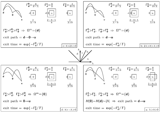
Figure 7: Summary of results for the Blume–Capel model.

3 Probabilistic cellular automata with self–interaction.

We have seen above how in the case of a three–state model as the Blume–Capel model competing metastable states shows up. In some sense this result is natural because the single site configuration space is three–state. In the framework of Probabilistic Cellular Automata it has been shown, see [10, 11, 12, 13], how competing metastable states arise in the context of a genuine two–state model.

Consider the two–dimensional torus $\Lambda=\{0,\dots,L-1\}^{2}$, with $L$ even, endowed with the Euclidean metric. Associate a variable $\sigma(x)=\pm 1$ with each site $x\in\Lambda$ and let $\Omega=\{-1,+1\}^{\Lambda}$ be the configuration space. Let $\beta>0$ and $\kappa,h\in[0,1]$. Consider the Markov chain $\sigma_{n}$, with $n=0,1,\dots$, on $\Omega$ with transition matrix

(6) $$p(\sigma,\eta)=\prod_{x\in\Lambda}p_{x,\sigma}\left(\eta(x)\right)\;\;\;\forall\sigma,\eta\in\Omega$$

where, for $x\in\Lambda$ and $\sigma\in\Omega$, $p_{x,\sigma}(\cdot)$ is the probability measure on $\{-1,+1\}$ defined as $p_{x,\sigma}(s)=1/[1+\exp\left\{-2\beta s(S_{\sigma}(x)+h)\right\}]$ with $s\in\{-1,+1\}$ and $S_{\sigma}(x)=\sum_{y\in\Lambda}K(x-y)\,\sigma(y)$ where $K(x-y)$ is $0$ if $|x-y|\geq 2$, $1$ if $|x-y|=1$, and $\kappa$ if $|x-y|=0$. The probability $p_{x,\sigma}(s)$ for the spin $\sigma(x)$ to be equal to $s$ depends only on the values of the spins of $\sigma$ in the five site cross centered at $x$. The metastable behavior of model (6) has been studied in Ref. [11] for $\kappa=0$ and in Ref. [10, 12] for $\kappa=1$.

The Markov chain (6) is a probabilistic cellular automata (PCA); the chain $\sigma_{n}$, with $n=0,1,\dots$, updates all the spins simultaneously and independently at any time. The chain is reversible with respect to the Gibbs measure $\mu(\sigma)=\exp\{-\beta H(\sigma)\}/Z$ with $Z=\sum_{\eta\in\Omega}\exp\{-\beta H(\eta)\}$ and

(7) $$H(\sigma)=-h\sum_{x\in\Lambda}\sigma(x)-\frac{1}{\beta}\sum_{x\in\Lambda}\log\cosh\left[\beta\left(S_{\sigma}(x)+h\right)\right]$$

that is detailed balance $p(\sigma,\eta)\,e^{-\beta H(\sigma)}=p(\eta,\sigma)\,e^{-\beta H(\eta)}$ holds and, hence, $\mu$ is stationary; $1/\beta$ is called the temperature and $h$ the magnetic field.

Although the dynamics is reversible w.r.t. the Gibbs measure associated to the Hamiltonian (7), the probability $p(\sigma,\eta)$ cannot be expressed in terms of $H(\sigma)-H(\eta)$, as usually happens for Glauber dynamics. Given $\sigma,\eta\in\Omega$, we define the energy cost

(8) $$\Delta(\sigma,\eta)=-\lim_{\beta\to\infty}\frac{\log p(\sigma,\eta)}{\beta}=\!\!\!\!\!\!\!\!\!\sum_{\genfrac{}{}{0.0pt}{}{x\in\Lambda:}{\eta(x)[S_{\sigma}(x)+h]<0}}\!\!\!\!\!\!\!\!\!2|S_{\sigma}(x)+h|$$

Note that $\Delta(\sigma,\eta)\geq 0$ and $\Delta(\sigma,\eta)$ is not necessarily equal to $\Delta(\eta,\sigma)$; it can be proven, see [12, Section 2.6], that

(9) $$e^{-\beta\Delta(\sigma,\eta)-\beta\gamma(\beta)}\leq p(\sigma,\eta)\leq e^{-\beta\Delta(\sigma,\eta)+\beta\gamma(\beta)}$$

with $\gamma(\beta)\to 0$ in the zero temperature limit $\beta\to\infty$. Hence, $\Delta$ can be interpreted as the cost of the transition from $\sigma$ to $\eta$ and plays the role that, in the context of Glauber dynamics, is played by the difference of energy.

In this context the ground states are those configurations on which the Gibbs measure $\mu$ concentrates when $\beta\to\infty$; hence, they can be defined as the minima of the energy

(10) $$E(\sigma)=\lim_{\beta\to\infty}H(\sigma)=-h\sum_{x\in\Lambda}\sigma(x)-\sum_{x\in\Lambda}|S_{\sigma}(x)+h|$$

For $X\subset\Omega$, we set $E(X)=\min_{\sigma\in X}E(\sigma)$. For $h>0$ the configuration ${\mathbf{u}}$, with ${\mathbf{u}}(x)=+1$ for $x\in\Lambda$, is the unique ground state, indeed each site contributes to the energy with $-h-(4+\kappa+h)$. For $h=0$, the ground states are the configurations such that all the sites contribute to the sum (10) with $4+\kappa$. Hence, for $\kappa\in(0,1]$, the sole ground states are the configurations ${\mathbf{u}}$ and ${\mathbf{d}}$, with ${\mathbf{d}}(x)=-1$ for $x\in\Lambda$. For $\kappa=0$, the configurations $\mathbf{c}^{\textrm{e}},\mathbf{c}^{\textrm{o}}\in\Omega$ such that $\mathbf{c}^{\textrm{e}}(x)=(-1)^{x_{1}+x_{2}}$ and $\mathbf{c}^{\textrm{o}}(x)=(-1)^{x_{1}+x_{2}+1}$ for $x=(x_{1},x_{2})\in\Lambda$ are ground states, as well. Notice that $\mathbf{c}^{\textrm{e}}$ and $\mathbf{c}^{\textrm{o}}$ are chessboard–like states with the pluses on the even and odd sub–lattices, respectively; we set $\mathbf{c}=\{\mathbf{c}^{\textrm{e}},\mathbf{c}^{\textrm{o}}\}$. Since the side length $L$ of the torus $\Lambda$ is even, then $E(\mathbf{c}^{\textrm{e}})=E(\mathbf{c}^{\textrm{o}})=E(\mathbf{c})$. By studying those energies as a function of $\kappa$ and $h$, recalling that periodic boundary conditions are considered, we get $E({\mathbf{u}})=-L^{2}(4+\kappa+2h)$, $E({\mathbf{d}})=-L^{2}(4+\kappa-2h)$, and $E(\mathbf{c})=-L^{2}(4-\kappa)$; hence $E(\mathbf{c})>E({\mathbf{d}})>E({\mathbf{u}})$ for $0<h<\kappa\leq 1$, $E(\mathbf{c})=E({\mathbf{d}})>E({\mathbf{u}})$ for $0<h=\kappa\leq 1$, and $E({\mathbf{d}})>E(\mathbf{c})>E({\mathbf{u}})$ for $0<\kappa<h\leq 1$.

In [13] the metastable behavior of this model has been studied with an heuristic argument very similar to the one developed in the Section 2 to discuss the metastable behavior of the Blume–Capel model. For the details we refer the interested reader to the quoted paper, we just mention here, that quite surprisingly results very similar to the ones obtained in the framework of the Blume–Capel model are found, provided the different parameters are interpreted according to the correspondences in Table 2.

Table 2: Correspondence between the Blume–Capel model and the PCA.

Blume–Capel	${\mathbf{u}}$	${\mathbf{d}}$	${\mathbf{0}}$	$h$	$\lambda$
PCA	${\mathbf{u}}$	${\mathbf{d}}$	$\mathbf{c}$	$h/2$	$\kappa/2$

Notice that the role of the zero state of the Blume–Capel model is played, in the context of the PCA, by the flip–flopping chessboard–like configurations. As (4) shows, the discussed results are valid in the limit $\beta\to\infty$. Their validity at finite temperature can be tested with Monte Carlo simulations, see the configurations in Figure 8 observed in a run of the dynamics of the PCA with the parameters specified in the caption and with starting configuration ${\mathbf{d}}$. On the left it is shown that if the self–interaction is present the nucleation of the plus phase is achieved directly; the plot on the right shows that, if the self–interaction is zero, than the chessboard–like phase is visited before the plus phase is nucleated.

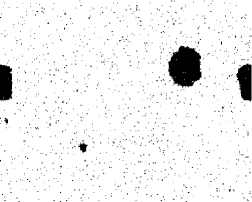
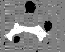
Figure 8: On the left, typical configuration of the PCA with $\kappa=1$; simulation performed on a $380\times 230$ torus with $\beta=0.7$. White and black points represent respectively minus and plus spins. On the right, the same with $\kappa=0$; the chessboard region looks grey.

References

- [1] E. Olivieri and M. E. Vares, Large deviations and metastability. Cambridge University Press, UK, 2004.
- [2] K. Huang, Statistical Mechanics. Wiley, 1987.
- [3] P.R. ten Wolde and D. Frenkel, Enhancement of Protein Crystal Nucleation by Critical Density Fluctuations, Science, 277 (1997) pp. 1975–1978.
- [4] G. Biroli and J. Kurchan, Metastable states in glassy systems, Phys. Rev. E, 64 (2001) pp. 016101(1–14).
- [5] M. Blume, Theory of the First–Order Magnetic Phase Change in , Phys. Rev., 141 (1966) pp. 517–524.
- [6] H.W. Capel, On the possibility of first–order phase transitions in Ising systems of triplet ions with zero-field splitting Physica, 32, (1966) pp. 966–988.
- [7] E.N.M. Cirillo and E. Olivieri, Metastability and nucleation for the Blume-Capel model. Different mechanisms of transition, J. Stat. Phys., 83 (1996) pp. 473–554.
- [8] T. Fiig, B.M. Gorman, P.A. Rikvold, and M.A. Novotny, Numerical transfer–matrix study of a model with competing metastable states, Phys. Rev. E, 50 (1994) pp. 1930–1947.
- [9] F. Manzo, F.R. Nardi, E. Olivieri, and E. Scoppola, On the essential features of metastability: tunnelling time and critical configurations, J. Stat. Phys., 115 (2004) pp. 591–642.
- [10] S. Bigelis, E.N.M. Cirillo, J.L. Lebowitz, and E.R. Speer, Critical droplets in metastable probabilistic cellular automata, Phys. Rev. E, 59 (1999) pp. 3935–3941.
- [11] E. N. M. Cirillo and F. R. Nardi, Metastability for the Ising model with a parallel dynamics, J. Stat. Phys., 110 (2003) pp. 183–217.
- [12] E.N.M. Cirillo, F.R. Nardi and C. Spitoni, Metastability for a reversible probabilistic cellular automata with self–interaction. J. Stat. Phys., 132 (2008) pp. 431–471.
- [13] E.N.M. Cirillo, F.R. Nardi and C. Spitoni, Competitive nucleation in reversible Probabilistic Cellular Automata with self–interaction. Phys. Rev. E, 78 (2008) pp. 040601(1–4).