Particle Acceleration in Advection-Dominated Accretion Disks with Shocks: Green’s Function Energy Distribution

Abstract

The distribution function describing the acceleration of relativistic particles in an advection-dominated accretion disk is analyzed using a transport formalism that includes first-order Fermi acceleration, advection, spatial diffusion, and the escape of particles through the upper and lower surfaces of the disk. When a centrifugally-supported shock is present in the disk, the concentrated particle acceleration occurring in the vicinity of the shock channels a significant fraction of the binding energy of the accreting gas into a population of relativistic particles. These high-energy particles diffuse vertically through the disk and escape, carrying away both energy and entropy and allowing the remaining gas to accrete. The dynamical structure of the disk/shock system is computed self-consistently using a model previously developed by the authors that successfully accounts for the production of the observed relativistic outflows (jets) in M87 and Sgr A^∗. This ensures that the rate at which energy is carried away from the disk by the escaping relativistic particles is equal to the drop in the radial energy flux at the shock location, as required for energy conservation. We investigate the influence of advection, diffusion, and acceleration on the particle distribution by computing the nonthermal Green’s function, which displays a relatively flat power-law tail at high energies. We also obtain the energy distribution for the particles escaping from the disk, and we conclude by discussing the spectrum of the observable secondary radiation produced by the escaping particles.

1 INTRODUCTION

Accretion flows onto supermassive black holes with mass $M\lower 1.72218pt\hbox{$\;\buildrel>\over{\scriptstyle\sim}\;$}10^{8}\,M_{\odot}$ are believed to power the high-energy emission observed from quasars and active galactic nuclei (AGNs), as discussed by Lynden-Bell (1969; see also Novikov & Thorne 1973; Rees 1984; and Ford et al. 1994). When the accretion rate is relatively low compared with the Eddington value, the flow is radiatively inefficient, and the gas temperature approaches the virial value. In this case the disk has an advection-dominated structure, and most of the binding energy is swallowed by the black hole (e.g., Narayan, Kato, & Honma 1997; Blandford & Begelman 1999; Becker, Subramanian, & Kazanas 2001; Becker & Le 2003). Despite the inefficiency of X-ray production in these sources, advection-dominated disks are luminous radio and $\gamma$-ray emitters, and they frequently display powerful bipolar jets of matter escaping from the central mass, presumably containing high-energy particles (e.g., Sambruna et al. 2004; Di Matteo et al. 2000; Allen, Di Matteo & Fabian 2000; Urry & Padovani 1995; Owen, Eilek, & Kassim 2000).

Although the effect of a standing shock in heating the gas in the post-shock region has been examined by a number of previous authors for both viscid (Chakrabarti & Das 2004; Lu, Gu, & Yuan 1999; Chakrabarti 1990) and inviscid (e.g., Lu & Yuan 1997, 1998; Yang & Kafatos 1995; Abramowicz & Chakrabarti 1990) disks, the implications of the shock for the acceleration of nonthermal particles in the disk have not been considered in detail before. However, a great deal of attention has been focused on particle acceleration in the vicinity of supernova-driven shock waves as a possible explanation for the observed cosmic-ray energy spectrum (Blandford & Ostriker 1978; Jones & Ellison 1991). In the present paper we consider the analogous process occurring in hot, advection-dominated accretion flows (ADAFs) around black holes. These disks are ideal sites for first-order Fermi acceleration at shocks because the plasma is collisionless, and therefore a small fraction of the particles can gain a great deal of energy by repeatedly crossing the shock. Shock acceleration in the disk therefore provides an intriguing possible explanation for the powerful outflows of relativistic particles observed in many radio-loud systems (Le & Becker 2004).

The idea of shock acceleration in the environment of AGNs was first suggested by Blandford & Ostriker (1978). Subsequently, Protheroe & Kazanas (1983) and Kazanas & Ellison (1986) investigated shocks in spherically-symmetric accretion flows as a possible explanation for the energetic radio and $\gamma$-radiation emitted by many AGNs. However, in these papers the acceleration of the particles was studied without the benefit of a detailed transport equation, and the assumption of spherical symmetry precluded the treatment of acceleration in disks. The state of the theory was advanced significantly by Webb & Bogdan (1987) and Spruit (1987), who employed a transport equation to solve for the distribution of energetic particles in a spherical accretion flow characterized by a self-similar velocity profile terminating at a standing shock. While more quantitative in nature than the earlier models, these solutions are not directly applicable to disks since the geometry is spherical and the velocity distribution is inappropriate. Hence none of these previous models can be used to develop a single, global, self-consistent picture for the acceleration of relativistic particles in an accretion disk containing a shock.

Accretion disks around black holes are not spherical, except perhaps in the innermost region, and therefore a transport equation written in cylindrical geometry is required in order to describe the acceleration of energetic particles in the accreting plasma. In this paper we develop a self-consistent cylindrically-symmetric model describing the acceleration of protons and/or electrons via first-order Fermi acceleration processes operating in a hot, advection-dominated accretion disk containing an isothermal shock. This is the third and final paper in a series studying the production of relativistic particles in ADAF disks with shocks. In Le & Becker (2004; hereafter Paper 1), we successfully applied our inflow/outflow model to explain the observed kinetic power of the outflows in M87 and Sgr A^∗, and in Le & Becker (2005; hereafter Paper 2), we discussed the detailed dynamics of ADAF disks containing isothermal shocks. Based on this dynamical model we can self-consistently compute the structure of the shocked disk and also the rate of escape of particles and energy from the disk at the shock location. In this paper we provide further details regarding the distribution in space and energy of the accelerated particles in the disk, and we also describe the energy distribution of the relativistic particles escaping from the disk at the shock location. Our focus here is on the computation of the Green’s function for monoenergectic particle injection, which describes in detail how the particles are advected, diffused, and accelerated within the disk, resulting in a nonthermal particle distribution with a high-energy power-law tail. We also discuss the spectrum of the observable secondary radiation produced by the escaping particles, including radio (synchrotron) as well as inverse-Compton X-ray and $\gamma$-ray emission, which provides a quantitative basis for developing observational tests of the model.

The first-order Fermi acceleration scenario that we focus on here (and in Papers 1 and 2) parallels the early studies of cosmic-ray acceleration in supernova shock waves. In analogy with the supernova case, we expect that shock acceleration in the disk will naturally produce a power-law energy distribution for the accelerated particles. Our earlier work in Paper 2 established that the first-order Fermi mechanism provides a very efficient means for accelerating the jet particles. In this paper, the solution for the Green’s function, $f_{{}_{\rm G}}(E,r)$, describing the evolution of monoenergetic seed particles injected into the disk, is obtained by solving the transport equation using the method of separation of variables. The eigenvalues and the corresponding spatial eigenfunctions are determined using a numerical approach because the differential equation obtained for the spatial function cannot be solved in closed form. The resulting solution for the Green’s function provides useful physical insight into how the relativistic particles are distributed in space and energy. We can also use the solution for $f_{{}_{\rm G}}(E,r)$ to check the self-consistency of the theory by comparing the numerical values obtained for the number and energy densities by integrating the Green’s function with those obtained in Paper 2 by directly solving the associated differential equations for these quantities.

The remainder of the paper is organized as follows. In § 2 we briefly review the inviscid dynamical model used to describe the structure of the ADAF disk/shock system. In § 3 we develop and solve the associated steady-state particle transport equation to obtain the solution for the Green’s function, $f_{{}_{\rm G}}(E,r)$, describing the evolution of monoenergetic seed particles injected from a source located at the shock radius, and in § 4 we evaluate the Green’s function using dynamical parameters appropriate for M87 and Sgr A^∗. In § 5 we discuss the observational implications of our results for the production of secondary radiation by the outflowing relativistic particles, and in § 6 we review our main conclusions.

2 ACCRETION DYNAMICS

It has been known for some time that inviscid accretion disks can display both shocked and shock-free (i.e., smooth) solutions depending on the values of the energy and angular momentum per unit mass in the gas supplied at a large radius (e.g., Chakrabarti 1989; Chakrabarti & Molteni 1993; Kafatos & Yang 1994; Lu & Yuan 1997; Das, Chattopadhyay, & Chakrabarti 2001). Shocks can also exist in viscous disks if the viscosity is relatively low (Chakrabarti 1996; Lu, Gu, & Yuan 1999), although smooth solutions are always possible for the same set of upstream parameters (Narayan, Kato, & Honma 1997; Chen, Abramowicz, & Lasota 1997). Hawley, Smarr, & Wilson (1984a, 1984b) have shown through general relativistic simulations that if the gas is falling with some rotation, then the centrifugal force can act as a “wall,” triggering the formation of a shock. Furthermore, the possibility that shock instabilities may generate the quasi-periodic oscillations (QPOs) observed in some sources containing black holes has been pointed out by Chakrabarti, Acharyya, & Molteni (2004), Lanzafame, Molteni, & Chakrabarti (1998), Molteni, Sponholz, & Chakrabarti (1996), and Chakrabarti & Molteni (1995). Nevertheless, shocks are “optional” even when they are allowed, and one is always free to construct models that avoid them. However, in general the shock solution possesses a higher entropy content than the shock-free solution, and therefore we argue based on the second law of thermodynamics that when possible, the shocked solution represents the preferred mode of accretion (Becker & Kazanas 2001; Chakrabarti & Molteni 1993).

The possible presence of shocks in hot ADAF disks with low viscosity motivated us to explore in Paper 2 the relationship between the dynamical structure of the disk/shock system and the possible acceleration of relativistic particles that can escape from the disk to power the outflows commonly observed from radio-loud accretion flows around both stellar-mass and supermassive black holes. The disk/shock/outflow model is depicted schematically in Figure 1. In this scenario, the gas is accelerated gravitationally toward the central mass, and experiences a shock transition due to an obstruction near the event horizon. The obstruction is provided by the “centrifugal barrier,” which is located between the inner and outer sonic points. Particles from the high-energy tail of the background Maxwellian distribution are accelerated at the shock discontinuity via the first-order Fermi mechanism, resulting in the formation of a nonthermal, relativistic particle distribution in the disk. The spatial transport of the energetic particles within the disk is a stochastic process based on a three-dimensional random walk through the accreting background gas. Consequently, some of the accelerated particles diffuse to the disk surface and become unbound, escaping through the upper and lower edges of the cylindrical shock to form the outflow, while others diffuse outward radially through the disk or advect across the event horizon into the black hole.

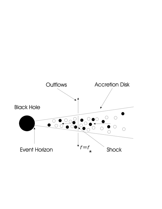
Figure 1: Schematic representation of the disk/shock/outflow model. The filled circles in the disk represent the accelerated particles, and the open circles represent the MHD scattering centers which advect with the background flow velocity. The seed particles are injected at the shock location.

2.1 Transport Rates

Becker & Le (2003) and Becker & Subramanian (2005) demonstrated that three integrals of the flow are conserved in viscous ADAF disks when outflows are not occurring. The three integrals correspond to the mass transport rate

$$\dot{M}=4\pi rH\rho\,u\ ,$$ (1)

the angular momentum transport rate

$$\dot{J}=\dot{M}r^{2}\,\Omega-\mathcal{G}\ ,$$ (2)

and the energy transport rate

$$\dot{E}=-\mathcal{G}\,\Omega+\dot{M}\left({1\over 2}\,v_{\phi}^{2}+{1\over 2}\,u^{2}+{P+U\over\rho}+\Phi\right)\ ,$$ (3)

where $\rho$ is the mass density, $\Omega$ is the angular velocity, ${\cal G}$ is the torque, $H$ is the disk half-thickness, $u$ is the positive radial inflow speed, $v_{\phi}=r\,\Omega$ is the azimuthal velocity, $U$ is the internal energy density, $P=(\gamma-1)\,U$ is the pressure, and

$$\Phi(r)\equiv{-GM\over r-r_{{}_{\rm S}}}$$ (4)

denotes the pseudo-Newtonian gravitational potential for a black hole with mass $M$ and Schwarzschild radius $r_{{}_{\rm S}}=2GM/c^{2}$ (Paczyński & Wiita 1980). Each of the various densities and velocities represents a vertical average over the disk structure. We also assume that the ratio of specific heats, $\gamma$, maintains a constant value throughout the flow. Note that all of the transport rates $\dot{M}$, $\dot{J}$, and $\dot{E}$ are defined to be positive for inflow.

The quantities $\dot{M}$ and $\dot{J}$ remain constant throughout the entire flow, and therefore they represent the rates at which mass and angular momentum, respectively, enter the black hole. The energy transport rate $\dot{E}$ also remains constant, except at the location of an isothermal shock if one is present in the disk. The torque ${\cal G}$ is related to the gradient of the angular velocity $\Omega$ via the usual expression (e.g., Frank et al. 2002)

$$\mathcal{G}=-4\pi r^{3}H\rho\,\nu{d\Omega\over dr}\ ,$$ (5)

where $\nu$ is the kinematic viscosity. The disk half-thickness $H$ is given by the standard hydrostatic prescription

$$H(r)={c_{s}\over\Omega_{\rm K}}\ ,$$ (6)

where $c_{s}$ represents the adiabatic sound speed, defined by

$$c_{s}(r)\equiv\left({\gamma P\over\rho}\right)^{1/2}\ ,$$ (7)

and $\Omega_{\rm K}$ denotes the Keplerian angular velocity of matter in a circular orbit at radius $r$ in the pseudo-Newtonian potential (eq. [4]), defined by

$$\Omega_{\rm K}^{2}(r)\equiv{GM\over r(r-r_{{}_{\rm S}})^{2}}={1\over r}{d\Phi\over dr}\ .$$ (8)

2.2 Inviscid Flow Equations

Following the approach taken in Paper 2, we focus here on the inviscid case since that allows the disk structure to be computed analytically, while retaining reasonable agreement with the dynamics of actual disks with low viscosities. We utilize the set of physical conservation equations employed by Chakrabarti (1989) and Abramowicz & Chakrabarti (1990), who investigated the structure of one-dimensional, inviscid, steady-state, axisymmetric accretion flows. In the inviscid limit, the torque ${\cal G}$ vanishes, and the angular momentum per unit mass transported through the disk is given by

$$\ell(r)\equiv{\dot{J}\over\dot{M}}=r^{2}\,\Omega(r)={\rm constant}\ .$$ (9)

We can combine equations (3) and (7) to show that the energy transported per unit mass in the inviscid case can be written as

$$\epsilon\equiv{\dot{E}\over\dot{M}}={1\over 2}\,u^{2}+{1\over 2}\,{\ell^{2}\over r^{2}}+{c_{s}^{2}\over\gamma-1}+\Phi\ ,$$ (10)

where we have also utilized the relation $\ell=rv_{\phi}$. The resulting disk/shock model depends on three free parameters, namely the energy transport per unit mass $\epsilon$, the specific heats ratio $\gamma$, and the specific angular momentum $\ell$. The value of $\epsilon$ will jump at the location of an isothermal shock if one exists in the disk, but the value of $\ell$ remains constant throughout the flow. This implies that the specific angular momentum of the particles escaping through the upper and lower surfaces of the cylindrical shock must be equal to the average value of the specific angular momentum for the particles remaining in the disk, and therefore the outflow exerts no torque on the disk (Becker, Subramanian, & Kazanas 2001).

The values of the energy transport parameter $\epsilon$ on the upstream and downstream sides of the isothermal shock at $r=r_{*}$ are denoted by $\epsilon_{-}$ and $\epsilon_{+}$, respectively. The condition $\epsilon_{-}>\epsilon_{+}$ must be satisfied as a consequence of the loss of energy through the upper and lower surfaces of the disk at the shock location. In order to satisfy global energy conservation, the rate at which energy escapes from the gas as it crosses the shock must be equal to the jet luminosity, $L_{\rm jet}$, and therefore we have

$$L_{\rm jet}\equiv-\Delta\dot{E}=-\dot{M}\,\Delta\epsilon\ \ \propto\ {\rm ergs\ s}^{-1}\ ,$$ (11)

where $\Delta$ denotes the difference between quantities on the downstream and upstream sides of the shock, so that $\Delta\epsilon=\epsilon_{+}-\epsilon_{-}<0$. The drop in $\epsilon$ at the shock has the effect of altering the transonic structure of the flow in the post-shock region, compared with the shock-free configuration (see Paper 2). In the inviscid case, the flow is purely adiabatic except at the location of an isothermal shock (if one is present), and therefore the pressure is related to the density profile via

$$P=D_{0}\,\rho^{\gamma}\ ,$$ (12)

where $D_{0}$ is a parameter related to the specific entropy that remains constant except at the location of a shock. The process of constructing a dynamical model for a specific disk/shock system begins with the selection of values for the fundamental parameters $\epsilon_{-}$, $\ell$, and $\gamma$. For given values of these three quantities, a unique flow structure can be obtained using the procedure discussed in §§ 3 and 4 of Paper 2, which yields a numerical solution for the inflow speed $u(r)$. Following Narayan, Kato, & Honma (1997), we shall assume an approximate equipartition between the gas and magnetic pressures, and therefore we set $\gamma=1.5$. The range of acceptable values for $\epsilon_{-}$ and $\ell$ is constrained by the observations of a specific object, as discussed in § 7 of Paper 2.

3 STEADY-STATE PARTICLE TRANSPORT

The gas in ADAF disks is hot and tenuous, and therefore essentially collisionless. In this situation, the relativistic particles diffuse mainly via collisions with magnetohydrodynamical (MHD) scattering centers (e.g., Alfvén waves), which control both the spatial transport and the acceleration of the particles. The magnetic scattering centers are advected along with the background flow, and therefore the shock width is expected to be comparable to the magnetic coherence length, $\lambda_{\rm mag}$. Particles from the high-energy tail of the background Maxwellian distribution are accelerated at the shock discontinuity via the first-order Fermi mechanism, resulting in the formation of a nonthermal, relativistic particle distribution in the disk. The probability of multiple shock crossings decreases exponentially with the number of crossings, and the mean energy of the particles increases exponentially with the number of crossings. This combination of factors naturally gives rise to a power-law energy distribution, which is a general characteristic of Fermi processes (Fermi 1954).

Two effects limit the maximum energy that can be achieved by the particles. First, at very high energies the particles will tend to lose energy to the waves due to recoil. Second, the mean free path $\lambda_{\rm mag}$ will eventually exceed the thickness of the disk as the particle energy is increased, resulting in escape from the disk without further acceleration. As a consequence of the random walk, some of the accelerated particles diffuse to the disk surface and become unbound, escaping through the upper and lower edges of the cylindrical shock to form the outflow, while others diffuse outward radially through the disk or advect across the event horizon into the black hole (see Fig. 1). Our goal in this paper is to analyze the Green’s function $f_{{}_{\rm G}}(E,r)$ in the disk based on the transport equation and the dynamical results discussed in Paper 2. We focus specifically on models 2 and 5 from Paper 2, which describe the disk structures for M87 and Sgr A^∗, respectively.

3.1 Transport Equation

The particle transport formalism we utilize includes advection, spatial diffusion, first-order Fermi acceleration, and particle escape. Our treatment of the Fermi process includes both the general compression related to the overall convergence of the accretion flow, as well as the enhanced compression that occurs at the shock. To avoid unnecessary mathematical complexity, we utilize a simplified model for the spatial transport in which only the radial ($r$) component is treated in detail. In this approach, the diffusion and escape of the particles in the vertical ($z$) direction is modeled using an escape-probability formalism. We will adopt the test-particle approximation utilized in Paper 2, meaning that the dynamical effect of the relativistic particle pressure on the flow structure is assumed to be negligible. This assumption is valid provided the pressure of the relativistic particles is much smaller than the background (thermal) pressure, which is verified for models 2 and 5 in § 8 of Paper 2. We also assume that the injection of the seed particles and the escape of the accelerated particles from the disk are both localized at the isothermal shock radius, which is consistent with the strong concentration of first-order Fermi acceleration in the vicinity of the shock.

The localization of the particle injection and escape at the shock radius allows us to make a direct connection between the jump in the energy flux in the disk at the shock location and the energy carried away by the escaping particles. This connection is essential in order to maintain self-consistency between the dynamical and transport calculations, as discussed in Paper 2. In a steady-state situation, the Green’s function, $f_{{}_{\rm G}}(E,r)$, representing the particle distribution resulting from the continual injection of monoenergetic seed particles from a source located at the shock radius ($r=r_{*}$) satisfies the transport equation (Becker 1992)

$${\partial f_{{}_{\rm G}}\over\partial t}=0=-\vec{\nabla}\cdot\vec{F}-{1\over 3E^{2}}{\partial\over\partial E}\left(E^{3}\,\vec{v}\cdot\vec{\nabla}f_{{}_{\rm G}}\right)+\dot{f}_{\rm source}-\dot{f}_{\rm esc}\ ,$$ (13)

where the specific flux $\vec{F}$ is evaluated using

$$\vec{F}=-\kappa\vec{\nabla}f_{{}_{\rm G}}-\vec{v}\,{E\over 3}\,{\partial f_{{}_{\rm G}}\over\partial E}\ ,$$ (14)

and the quantities $E$, $\kappa$, and $\vec{v}$ represent the particle energy, the spatial diffusion coefficient, and the vector velocity, respectively. The velocity has components given by $\vec{v}=v_{r}\hat{r}+v_{z}\hat{z}+v_{\phi}\,\hat{\phi}$, with $v_{r}=-u<0$ since we are dealing with inflow.

The injection of the monoenergetic seed particles is described by the function

$$\dot{f}_{\rm source}={\dot{N}_{0}\,\delta(E-E_{0})\,\delta(r-r_{*})\over(4\pi E_{0})^{2}\,r_{*}\,H_{*}}\ ,$$ (15)

where $E_{0}$ is the energy of the injected particles, $\dot{N}_{0}$ is the particle injection rate, and $H_{*}\equiv H(r_{*})$ represents the half-thickness of the disk at the shock location. The escape of the particles through the upper and lower surfaces of the disk is represented by the term

$$\dot{f}_{\rm esc}=A_{0}\,c\,\delta(r-r_{*})\,f_{{}_{\rm G}}\ ,$$ (16)

where the dimensionless parameter $A_{0}$ is computed using (see Appendix B of Paper 2)

$$A_{0}=\left(3\kappa_{*}\over cH_{*}\right)^{2}<1\ ,$$ (17)

and $\kappa_{*}\equiv(\kappa_{-}+\kappa_{+})/2$ denotes the mean value of the spatial diffusion coefficient at the shock radius. The subscripts “-” and “+” will be used to denote quantities measured just upstream and just downstream from the shock, respectively. The condition $A_{0}<1$ is required for the validity of the diffusive treatment of the vertical escape employed in our approach.

In order to compute the Green’s function $f_{{}_{\rm G}}(E,r)$, we must specify the injection energy of the seed particles $E_{0}$ as well as their injection rate $\dot{N}_{0}$. Following the approach taken in Paper 2, we set the injection energy using $E_{0}=0.002\,$ergs, which corresponds to an injected Lorentz factor $\Gamma_{0}\equiv E_{0}/(m_{p}\,c^{2})\sim 1.3$, where $m_{p}$ is the proton mass. Particles injected with energy $E_{0}$ are subsequently accelerated to much higher energies due to repeated shock crossings. We find that the speed of the injected particles, $v_{0}=c\,(1-\Gamma_{0}^{-2})^{1/2}$, is several times larger than the mean ion thermal velocity at the shock location, $v_{\rm rms}=(3kT_{*}/m_{p})^{1/2}$, where $T_{*}$ is the ion temperature at the shock. The seed particles are therefore picked up from the high-energy tail of the local Maxwellian distribution. With $E_{0}$ specified, we can compute the particle injection rate $\dot{N}_{0}$ using the energy conservation condition

$$\dot{N}_{0}\,E_{0}=-\dot{M}\,\Delta\epsilon\ \ \propto\ {\rm ergs\ s}^{-1}\ ,$$ (18)

where $\Delta\epsilon<0$ represents the jump in the energy transport per unit mass as the plasma crosses the shock (see eqs. [10] and [11]). This relation ensures that the energy injection rate for the seed particles is equal to the energy loss rate for the background gas at the isothermal shock location.

The total number and energy densities of the relativistic particles, denoted by $n_{r}$ and $U_{r}$, respectively, are related to the Green’s function via

$$n_{r}(r)=\int_{0}^{\infty}4\pi E^{2}\,f_{{}_{\rm G}}(E,r)\,dE\ ,\ \ \ \ \ U_{r}(r)=\int_{0}^{\infty}4\pi E^{3}\,f_{{}_{\rm G}}(E,r)\,dE\ ,$$ (19)

which determine the normalization of $f_{{}_{\rm G}}$. Equations (13) and (14) can be combined to obtain the alternative form

$$\vec{v}\cdot\vec{\nabla}f_{{}_{\rm G}}={E\over 3}\,{\partial f_{{}_{\rm G}}\over\partial E}\,\vec{\nabla}\cdot\vec{v}+\vec{\nabla}\cdot\left(\kappa\,\vec{\nabla}f_{{}_{\rm G}}\right)+\dot{f}_{\rm source}-\dot{f}_{\rm esc}\ ,$$ (20)

where the left-hand side represents the co-moving (advective) time derivative and the terms on the right-hand side describe first-order Fermi acceleration, spatial diffusion, the particle source, and the escape of particles from the disk at the shock location, respectively. Note that escape and particle injection are localized to the shock radius due to the presence of the $\delta$-functions in equations (15) and (16). Our focus here is on the first-order Fermi acceleration of relativistic particles at a standing shock in an accretion disk, and therefore equation (20) does not include second-order Fermi processes that may also occur in the flow due to MHD turbulence (e.g., Schlickeiser 1989a,b; Subramanian, Becker, & Kazanas 1999; Becker et al. 2006). Since no energy loss mechanisms are included in the model, all of the particles injected with energy $E_{0}$ will experience an increase in energy.

Under the assumption of cylindrical symmetry, equations (15), (16), and (20) can be combined to obtain

$$v_{r}{\partial f_{{}_{\rm G}}\over\partial r}+v_{z}{\partial f_{{}_{\rm G}}\over\partial z} - {E\over 3}\,{\partial f_{{}_{\rm G}}\over\partial E}\left[{1\over r}{d\over dr}\left(rv_{r}\right)+{dv_{z}\over dz}\right]-{1\over r}{\partial\over\partial r}\left(r\kappa{\partial f_{{}_{\rm G}}\over\partial r}\right)$$ (21)

$$= {\dot{N}_{0}\,\delta(E-E_{0})\,\delta(r-r_{*})\over(4\pi E_{0})^{2}\,r_{*}H_{*}}-A_{0}\,c\,\delta(r-r_{*})\,f_{{}_{\rm G}}\ ,$$

where the escape of particles from the disk is described by the final term on the right-hand side. We focus here on the vertically-integrated form of the transport equation, which can be written as (see Paper 2, Appendix A)

$$-Hu{\partial f_{{}_{\rm G}}\over\partial r} = -{1\over r}\,{d\over dr}(rHu)\,{E\over 3}\,{\partial f_{{}_{\rm G}}\over\partial E}+{1\over r}{\partial\over\partial r}\left(rH\kappa\,{\partial f_{{}_{\rm G}}\over\partial r}\right)$$ (22)

$$+ {\dot{N}_{0}\,\delta(E-E_{0})\,\delta(r-r_{*})\over(4\pi E_{0})^{2}r_{*}}-A_{0}\,c\,H_{*}\,\delta(r-r_{*})\,f_{{}_{\rm G}}\ ,$$

where $u=-v_{r}$ and $f_{{}_{\rm G}}$ and $\kappa$ are vertically averaged quantities. Due to the presence of the velocity derivative on the right-hand side of equation (22), the first-order Fermi acceleration of the particles is most pronounced near the shock, where $u$ is discontinuous. In the vicinity of the shock, we find that

$${du\over dr}\to(u_{-}-u_{+})\,\delta(r-r_{*})\ ,\ \ \ \ \ r\to r_{*}\ ,$$ (23)

where $u_{-}$ and $u_{+}$ denote the positive inflow speeds just upstream and downstream from the shock, respectively. The velocity jump condition appropriate for an isothermal shock is (see Paper 2)

$${u_{+}\over u_{-}}={1\over\gamma\,{\cal M}_{-}^{2}}\ ,$$ (24)

where ${\cal M}_{-}$ is the incident Mach number on the upstream side of the shock. Although the Fermi acceleration of the particles is concentrated at the shock, the rest of the disk also contributes to the particle acceleration because of the general convergence of the MHD waves in the accretion flow.

In order to close the system of equations and solve for the Green’s function using equation (22), we must also specify the radial variation of the diffusion coefficient $\kappa$. The behavior of $\kappa$ can be constrained by considering the fundamental physical principles governing accretion onto a black hole, which we have demonstrated in Paper 2. The precise functional form for the spatial variation of $\kappa$ is not completely understood in the accretion disk environment. In order to obtain a mathematically tractable set of equations with a reasonable physical behavior, we utilize the general form (see Paper 2, § 5)

$$\kappa(r)=\kappa_{0}\,u(r)\,r_{{}_{\rm S}}\left({r\over r_{{}_{\rm S}}}-1\right)^{2}\ ,$$ (25)

where $\kappa_{0}>0$ is a dimensionless constant that can be computed for a given source based on energy considerations (see § 4). Due to the appearance of the radial speed $u$ in equation (25), we note that $\kappa$ exhibits a jump at the shock. This is expected on physical grounds since the MHD waves that scatter the ions are swept along with the thermal background flow, and therefore they should also experience a density compression at the shock. We also point out that the dimensionless escape parameter $A_{0}$ can be evaluated by combining equations (17) and (25), which yields

$$A_{0}=\left({3\kappa_{0}u_{*}r_{{}_{\rm S}}\over cH_{*}}\right)^{2}\left({r_{*}\over r_{{}_{\rm S}}}-1\right)^{4}<\,1\ ,$$ (26)

where $u_{*}\equiv(u_{-}+u_{+})/2$ denotes the mean value of the inflow speed at the shock location. Note that the value of the diffusion parameter $\kappa_{0}$ is constrained by the inequality in equation (26).

3.2 Separation of Variables

For values of the particle energy $E>E_{0}$, the source term in equation (22) vanishes and the remaining equation is separable in energy and space using the functions

$$f_{{}_{n}}(E,r)=\left(E\over E_{0}\right)^{-\lambda_{n}}\,Y_{n}(r)\ ,$$ (27)

where $\lambda_{n}$ are the eigenvalues, and the spatial eigenfunctions $Y_{n}(r)$ satisfy the second-order ordinary differential equation

$$-Hu{dY_{n}\over dr}={\lambda_{n}\over 3r}{d\over dr}(rHu)\,Y_{n}+{1\over r}{d\over dr}\left(rH\kappa\,{dY_{n}\over dr}\right)-A_{0}\,c\,H_{*}\,\delta(r-r_{*})\,Y_{n}\ .$$ (28)

The eigenvalues $\lambda_{n}$ are determined by applying suitable boundary conditions to the spatial eigenfunctions, as discussed below. Once a numerical solution for the inflow speed $u(r)$ has been obtained following the procedures described in Paper 2, we can compute $H(r)$ and $\kappa(r)$ using equations (6) and (25), respectively. Since the coefficients in equation (28) cannot be represented in closed form, analytical solutions cannot be obtained and therefore the eigenfunctions $Y_{n}(r)$ must be determined numerically. Away from the shock ($r\neq r_{*}$), equation (28) reduces to

$${d^{2}Y_{n}\over dr^{2}}+\left[{d\ln(rH\kappa)\over dr}+{u\over\kappa}\right]{dY_{n}\over dr}+{\lambda_{n}uY_{n}\over 3\,\kappa}\,{d\ln(rHu)\over dr}=0\ ,$$ (29)

which can be rewritten as

$${d^{2}Y_{n}\over dr^{2}}+\left[{d\ln(rHu)\over dr}+{2\over r-r_{{}_{\rm S}}}+{r_{{}_{\rm S}}\over\kappa_{0}(r-r_{{}_{\rm S}})^{2}}\right]{dY_{n}\over dr}+{\lambda_{n}r_{{}_{\rm S}}Y_{n}\over 3\kappa_{0}(r-r_{{}_{\rm S}})^{2}}\,{d\ln(rHu)\over dr}=0\ ,$$ (30)

where we have used equation (25) to substitute for $\kappa$. Once a solution for the inflow speed $u(r)$ has been determined using the procedure described in § 2, the variation of the disk half-thickness $H(r)$ can be computed by combining equations (1), (6), (7), and (12). The result obtained is

$$H(r)={1\over\Omega_{\rm K}(r)}\left[r^{3/2}(r-r_{{}_{\rm S}})\,u(r)\over K\right]^{(1-\gamma)/(1+\gamma)}\ ,$$ (31)

where $\Omega_{\rm K}$ is given by equation (8) and $K$ is the “entropy parameter”, which remains constant except at the location of an isothermal shock if one is present in the flow (see Paper 2 and Becker & Le 2003). By utilizing the solutions obtained for $u(r)$ and $H(r)$, we are able to compute all of the coefficients in equation (30), which allows us to solve numerically for the spatial eigenfunctions $Y_{n}(r)$.

3.3 Eigenvalues and Eigenfunctions

The global solution for the eigenfunction $Y_{n}(r)$ must satisfy continuity and derivative jump conditions associated with the presence of the shock/source at radius $r=r_{*}$. By integrating equation (28) with respect to radius in the vicinity of the shock, we find that

$$\Delta[Y_{n}] = 0\ ,$$ (32)

$$\Delta\left[\left({\lambda_{n}\over 3}\,u\,Y_{n}+\kappa\,{dY_{n}\over dr}\right)\right] = -cA_{0}Y_{n}(r_{*})\ ,$$ (33)

where the symbol $\Delta$ denotes the difference between postshock and preshock quantities, and we have made use of the fact that $H$ is continuous across the isothermal shock. Equations (32) and (33) establish that $Y_{n}(r)$ must be continuous at the shock location, and its derivative must display a jump there.

Since the spatial eigenfunctions $Y_{n}(r)$ satisfy the second-order linear differential equation (30), we must also impose two boundary conditions in order to determine the global solutions and the associated eigenvalues $\lambda_{n}$. The required conditions can be developed based on our knowledge of the dynamical structure of the disk near the event horizon ($r=r_{{}_{\rm S}}$) and at large radii (see Becker & Le 2003 and § 4 of Paper 2). By utilizing the Frobenius expansion method to identify the dominant terms in equation (30), we find that the global solutions for the spatial eigenfunctions can be written as

$$Y_{n}(r)=\left\{\begin{array}[]{ll}G^{\rm in}_{n}(r)&,\ \ r\leq r_{*}\ ,\\ \\ a_{n}G^{\rm out}_{n}(r)&,\ \ r\geq r_{*}\ ,\end{array}\right.$$

where $a_{n}$ is a matching constant and $G^{\rm in}_{n}(r)$ and $G^{\rm out}_{n}(r)$ denote the fundamental solutions to equation (30) possessing the asymptotic behaviors

$$\begin{array}[]{ll}G^{\rm in}_{n}(r)\to\ g^{\rm in}_{n}(r)\equiv\left({r\over r_{{}_{\rm S}}}-1\right)^{-\lambda_{n}/(3\gamma+3)}&,\ \ r\to r_{{}_{\rm S}}\ ,\\ \\ G^{\rm out}_{n}(r)\to\ g^{\rm out}_{n}(r)\equiv\left({r\over r_{{}_{\rm S}}}\right)^{-1}&,\ \ r\to\infty\ ,\end{array}$$

at small and large radii, respectively. The value of $a_{n}$ is determined using the continuity condition (see eq. [32]), which yields

$$a_{n}={G^{\rm in}_{n}(r_{*})\over G^{\rm out}_{n}(r_{*})}\ .$$ (34)

The validity of the asymptotic forms in equations (3.3) is verified in § 4.1 via comparison with the numerical solutions obtained for the spatial eigenfunctions.

We use a bi-directional integration scheme to solve for the eigenvalues $\lambda_{n}$ based on the boundary conditions in equations (3.3). The value of $\lambda_{n}$ is iterated using a bisection method until the Wronskian of the inner and outer solutions vanishes at a matching radius located in the postshock region. Once a particular eigenvalue has been determined to the required accuracy, the matching constant $a_{n}$ is computed using equation (34). This procedure is repeated until the desired number of eigenvalues and eigenfunctions have been obtained. The sequences of eigenvalues associated with the model 2 (M87) and model 5 (Sgr A^∗) parameters are plotted in Figure 2. Note that $\lambda_{1}\sim 4$ in all cases, indicating that the acceleration is quite efficient, in analogy with the case of cosmic-ray acceleration (e.g., Blandford & Ostriker 1978). The first two eigenvalues in models 2 and 5 are $\lambda_{1}=4.165$, $\lambda_{2}=6.415$ and $\lambda_{1}=4.180$, $\lambda_{2}=6.344$, respectively. It follows that at high energies the power-law slope of the energy distribution is dominated by the first eigenvalue $\lambda_{1}$, since all of the subsequent eigenvalues are much larger (see Fig. 2).

Figure 2: Eigenvalues for model 2 (M87; filled squares) and model 5 (Sgr A^∗; filled circles).

3.4 Eigenfunction Orthogonality

We can establish several useful general properties of the eigenfunctions by rewriting equation (30) in the Sturm-Liouville form

$${d\over dr}\left[S(r)\,{dY_{n}\over dr}\right]+\lambda_{n}\,\omega(r)\,Y_{n}(r)=0\ ,$$ (35)

where

$$S(r)\equiv{rH\kappa\over r_{*}H_{*}\kappa_{*}}\ \exp\left\{{1\over\kappa_{0}}\left[\left({r_{*}\over r_{{}_{\rm S}}}-1\right)^{-1}-\left({r\over r_{{}_{\rm S}}}-1\right)^{-1}\right]\right\}\ ,$$ (36)

and the weight function $\omega(r)$ is defined by

$$\omega(r)\equiv{u\,S\over 3\,\kappa}\,{d\ln(rHu)\over dr}\ .$$ (37)

Note that $\omega(r)$ displays a $\delta$-function discontinuity at the shock through its dependence on the derivative of $u(r)$. In the vicinity of the shock, we can combine equations (23), (36), and (37) to show that

$$\omega(r)\to\left({u_{-}-u_{+}\over 3\kappa_{*}}\right)\delta(r-r_{*})\ ,\ \ \ \ \ r\to r_{*}\ .$$ (38)

Based on the boundary conditions satisfied by the spatial eigenfunctions $Y_{n}(r)$ (see eqs. [3.3]), we demonstrate in Appendix A that the eigenfunctions satisfy the orthogonality relation

$$\int^{\infty}_{r_{{}_{\rm S}}}Y_{n}(r)\,Y_{m}(r)\,\omega(r)\,dr=0\ ,\ \ \ \ \ m\neq n\ .$$ (39)

3.5 Eigenfunction Expansion

We have established that $Y_{n}(r)$ is the solution to a standard Sturm-Liouville problem, and therefore it follows that the set of eigenfunctions is complete. Consequently, the Green’s function $f_{{}_{\rm G}}(E,r)$ can be represented using the eigenfunction expansion (see eq. [27])

$$f_{{}_{\rm G}}(E,r)=\sum^{N_{\rm max}}_{n=1}b_{n}Y_{n}(r)\left(E\over E_{0}\right)^{-\lambda_{\rm n}}\ ,\ \ \ \ \ E\geq E_{0}\ ,$$ (40)

where $b_{n}$ are the expansion coefficients (with either positive or negative signs) and the value of $N_{\rm max}$ is established by analyzing the term-by-term convergence of the series. We utilize the value $N_{\rm max}=10$ in our numerical examples, which generally yields an accuracy of at least three decimal digits. Note that $f_{{}_{\rm G}}(E,r)=0$ for all $E<E_{0}$ because no deceleration processes are included in the particle transport model.

The expansion coefficients $b_{1},b_{2},b_{3},\ldots$ can be calculated by utilizing the orthogonality of the spatial eigenfunctions. At the source energy, $E=E_{0}$, equation (40) reduces to

$$f_{{}_{\rm G}}(E_{0},r)=\sum^{N_{\rm max}}_{m=1}b_{m}\,Y_{m}(r)\ .$$ (41)

Multiplying each side of this expression by the product $Y_{n}(r)\,\omega(r)$ and integrating from $r=r_{{}_{\rm S}}$ to $r=\infty$ yields

$$\int^{\infty}_{r_{{}_{\rm S}}}f_{{}_{\rm G}}(E_{0},r)\,Y_{n}(r)\,\omega(r)\,dr=\sum^{N_{\rm max}}_{m=1}b_{m}\int^{\infty}_{r_{{}_{\rm S}}}Y_{m}(r)\ Y_{n}(r)\,\omega(r)\,dr\ .$$ (42)

Based on the orthogonality of the eigenfunctions, as expressed by equation (39), we note that only the $m=n$ term survives on the right-hand side of equation (42), and we therefore obtain

$$\int^{\infty}_{r_{{}_{\rm S}}}f_{{}_{\rm G}}(E_{0},r)\,Y_{n}(r)\,\omega(r)\,dr=b_{n}\int^{\infty}_{r_{{}_{\rm S}}}Y^{2}_{n}(r)\,\omega(r)\,dr\ .$$ (43)

Solving this expression for the expansion coefficient $b_{n}$ yields

$$b_{n}={\int^{\infty}_{r_{{}_{\rm S}}}f_{{}_{\rm G}}(E_{0},r)\,Y_{n}(r)\,\omega(r)\,dr\over{\cal I}_{n}}\ ,$$ (44)

where the quadratic normalization integrals, ${\cal I}_{n}$, are defined by

$${\cal I}_{n}\equiv\int^{\infty}_{r_{{}_{\rm S}}}Y^{2}_{n}(r)\,\omega(r)\,dr\ .$$ (45)

To complete the calculation of the expansion coefficients, we need to evaluate the distribution function at the source energy, $f_{{}_{\rm G}}(E_{0},r)$. This can be accomplished by using equation (23) to substitute for the velocity derivative in equation (22) and then integrating with respect to $E$ in a small range around the injection energy $E_{0}$, which yields

$$f_{{}_{\rm G}}(E_{0},r)=\left\{\begin{array}[]{ll}\displaystyle{3\dot{N}_{0}\over(4\pi)^{2}E_{0}^{3}\,r_{*}H_{*}(u_{-}-u_{+})}\ ,&r=r_{*}\ ,\\[12.0pt] \displaystyle{0}\ ,&r\neq r_{*}\ .\end{array}\right.$$ (46)

Although the source term in the transport equation (21) is a delta function, we note that the Green’s function evaluated at the injection energy $E_{0}$ is not a delta function. Instead, as indicated by equation (46), we find that the Green’s function at the injection energy is zero for radii away from the shock, and it is equal to a finite value at the shock ($r=r_{*}$). From a physical point of view, this reflects the fact that the particle injection occurs at the shock location in our model. The strong acceleration experienced by the particles at the shock eliminates the appearance of a delta-function behavior in the resulting Green’s function. It is interesting to compare this with the behavior observed in the case of particle acceleration in a plane-parallel supernova shock wave, which was analyzed in detail by Blandford & Ostriker (1978). Our results are similar to theirs, except that the Blandford & Ostriker Green’s function evaluated at the injection energy $E_{0}$ has a finite value at all locations in the flow, because there is no convergence in the plasma surrounding the plane-parallel supernova shock wave. However, in our model, the plasma converges at all radii in the accretion flow (not just at the shock), and this additional particle acceleration causes the Green’s function to vanish at the injection energy for all $r\neq r_{*}$.

Utilizing equation (46) to substitute for $f_{{}_{\rm G}}(E_{0},r)$ in equation (44) and carrying out the integration, we obtain

$$b_{n}={\dot{N}_{0}\,Y_{n}(r_{*})\over(4\pi)^{2}E_{0}^{3}\,r_{*}H_{*}\kappa_{*}{\cal I}_{n}}\ ,$$ (47)

where we have made use of the fact that the weight function $\omega(r)$ has a $\delta$-function behavior close to the shock (see eq. [38]). The singular nature of the weight function also needs to be considered when computing the normalization integrals ${\cal I}_{n}$ defined in equation (45). By combining equations (38) and (45), we find that

$${\cal I}_{n}=\lim_{\epsilon\to 0}\int_{r_{{}_{\rm S}}}^{r_{*}-\epsilon}\omega(r)\,Y^{2}_{n}(r)\,dr+\int_{r_{*}+\epsilon}^{\infty}\omega(r)\,Y^{2}_{n}(r)\,dr+\left(u_{-}-u_{+}\over 3\kappa_{*}\right)Y_{n}^{2}(r_{*})\ ,$$ (48)

and we shall use this expression to evaluate the normalization integrals.

4 ASTROPHYSICAL APPLICATIONS

In Paper 2 we investigated the acceleration of particles in an inviscid ADAF disk containing an isothermal shock. For a given source with a known black hole mass $M$, accretion rate $\dot{M}$, and jet kinetic power $L_{\rm jet}$, we found that a family of flow solutions can be obtained, with each solution corresponding to a different value of the diffusion parameter $\kappa_{0}$ (see eq. [25]). We concluded that the upstream energy flux, $\epsilon_{-}$, is maximized for a certain value of $\kappa_{0}$, and we adopted that particular value for $\kappa_{0}$ in our models for M87 and Sgr A^∗ in Paper 2. In Table 1 we list the values of the parameters $M$, $\dot{M}$, $L_{\rm jet}$, $\epsilon_{-}$, $\ell$, $\epsilon_{+}$, $r_{*}$, and $u_{*}$ associated with models 2 and 5, which describe M87 and Sgr A^∗, respectively.

Figure 3: The fundamental solutions to eq. (28) $G_{1}^{\rm in}(r)$ and $G_{1}^{\rm out}(r)$ (solid lines) for model 2 (M87) are compared with the corresponding asymptotic solutions $g_{1}^{\rm in}(r)$ and $g_{1}^{\rm out}(r)$ (dashed lines) in panels a and b, respectively (see eqs. [3.3]). The associated global solution for the first eigenfunction $Y_{1}(r)$ (eq. [3.3]) is plotted in panel c. The shock location at $r=r_{*}$ is indicated.

Table 1: Disk Structure Parameters

Source	Model	$M\atop(M_{\odot})$	$\dot{M}\atop(M_{\odot}\rm\ yr^{-1})$	$L_{\rm jet}\atop\rm(ergs\ s^{-1})$	$\epsilon_{-}$	$\ell$	$\epsilon_{+}$	$r_{*}$	$\mbox{\it\scriptsize u}_{*}\over\mbox{\it\scriptsize c}$
M87	2	$3.0\times 10^{9}$	$1.3\times 10^{-1}$	$5.5\times 10^{43}$	$1.527\times 10^{-3}$	3.1340	$-5.746\times 10^{-3}$	21.654	0.108
Sgr A∗	5	$2.6\times 10^{6}$	$8.8\times 10^{-7}$	$5.0\times 10^{38}$	$1.229\times 10^{-3}$	3.1524	$-8.749\times 10^{-3}$	15.583	0.124

Note. – All quantities are expressed in gravitational units ($GM=c=1$) except as indicated.

4.1 Numerical Solutions for the Eigenfunctions

Figure 4: Same as Figure 3 but for model 5, which describes Sgr A^∗.

Figure 5: Results for the relativistic particle Green’s function $f_{{}_{\rm G}}(E,r)$ in $\rm ergs^{-3}\,cm^{-3}$ computed using eq. (40) for (a) M87 (model 2), and (b) Sgr A^∗(model 5). The value of the radius $r$ in units of $GM/c^{2}$ is indicated for each curve, with $r=r_{*}$ denoting the shock location.

Figure 6: Plots of (a) the relativistic particle number density and (b) the relativistic particle energy density in cgs units for model 2, which describes M87. The solid lines represent the solutions computed by numerically integrating the associated differential equations, and the filled circles represent the corresponding results obtained by integrating the Green’s function using eqs. (49). The location of the shock at $r=r_{*}$ is indicated. Note the close agreement between the results, which confirms the accuracy of our computational model.

In order to compute the Green’s function $f_{{}_{\rm G}}(E,r)$, we must first solve for the eigenvalues $\lambda_{n}$ and eigenfunctions $Y_{n}(r)$ following the procedures described in §§ 3.3 and 3.4 based on equation (30). Once the eigenvalues and eigenfunctions have been determined, we can compute the expansion coefficients $b_{n}$ using equation (47), after which $f_{{}_{\rm G}}(E,r)$ is evaluated using equation (40). In Figure 3 we compare the fundamental asymptotic solutions $G_{n}^{\rm in}(r)$ and $G_{n}^{\rm out}(r)$ with the asymptotic solutions $g_{n}^{\rm in}(r)$ and $g_{n}^{\rm out}(r)$ for model 2 with $n=1$ (see eqs. [3.3]). The corresponding results for model 5 are plotted in Figure 4. The excellent agreement between the $G(r)$ and $g(r)$ functions confirms the validity of the asymptotic relations we have employed near the event horizon and also at large radii. Figures 3 and 4 also include plots of the global solutions for the first eigenfunction $Y_{1}(r)$ associated with models 2 and 5, respectively (see eq. [3.3]). Note that the global solutions display a derivative jump at the shock location, as required according to equation (33).

4.2 Green’s Function Particle Distribution

We can combine our results for the eigenvalues, eigenfunctions, and expansion coefficients to evaluate the Green’s function $f_{{}_{\rm G}}(E,r)$ using equation (40). In Figures 5a and 5b we plot $f_{{}_{\rm G}}(E,r)$ as a function of the particle energy $E$ at various radii $r$ in the disk for models 2 and 5, respectively. Note that at the injection energy ($E=E_{0}$), the Green’s function is equal to zero except at the source/shock radius, $r=r_{*}$, in agreement with equation (46). This reflects the fact that the particles are rapidly accelerated after they are injected, and therefore all particles have energy $E>E_{0}$ once they propagate away from the shock location. The positive slopes observed at low energies when $r\neq r_{*}$ result from the summation of terms with either positive or negative expansion coefficients $b_{n}$ (see § 3.5). At energies above the turnover, the spectrum has a power-law shape determined by the first eigenvalue, $\lambda_{1}\sim 4$ (see Fig. 2). The relatively flat slope of the Green’s function above the turnover reflects the high efficiency of the particle acceleration in the shocked disk. By contrast, in situations involving weak acceleration, the Green’s function has a strong peak at the injection energy surrounded by steep wings (e.g., Titarchuk & Zannias 1998).

In Paper 2 we established that most of the injected particles are advected inward by the accreting MHD waves, eventually crossing the event horizon into the black hole. Hence only a small fraction of the particles are able to diffuse upstream to larger radii, which is confirmed by the strong attenuation of the particle spectrum with increasing $r$ apparent in Figure 5. The particles in the inner region ($r<r_{*}$) exhibit the greatest overall energy gain because they are able to cross the shock multiple times, and they also experience the strong compression of the flow near the event horizon. This is consistent with the results for the mean energy distribution, $\langle E\rangle\equiv U_{r}/n_{r}$, plotted in Figure 9 of Paper 2.

4.3 Number and Energy Density Distributions

In our numerical examples, we have generated results for the Green’s function $f_{{}_{\rm G}}(E,r)$ by summing the first ten eigenfunctions using equation (40). Once the Green’s function energy distribution has been determined at a given radius, we can integrate it with respect to the particle energy $E$ to obtain the corresponding values for the number and energy densities. By combining equations (19) and (40) and integrating term-by-term, we obtain

$$n^{\rm G}_{r}(r)\equiv 4\pi E_{0}^{3}\sum^{N_{\rm max}}_{n=1}{b_{n}Y_{n}(r)\over\lambda_{n}-3}\ ,\ \ \ \ \ U^{\rm G}_{r}(r)\equiv 4\pi E_{0}^{4}\sum^{N_{\rm max}}_{n=1}{b_{n}Y_{n}(r)\over\lambda_{n}-4}\ .$$ (49)

Equations (49) provide an important tool for checking the self-consistency of our entire formalism. This is accomplished by comparing the results for the number and energy densities computed using equations (49) with the corresponding values obtained by directly solving the differential equations for $n_{r}$ and $U_{r}$ using the method developed in Paper 2. In principle, the two sets of results should agree closely if our procedure for computing $f_{{}_{\rm G}}(E,r)$ is robust. We compare the model 2 results obtained for $n_{r}$ and $U_{r}$ in Paper 2 with those computed using equations (49) in Figure 6. The corresponding comparison for model 5 is carried out in Figure 7. Note the close agreement between the two sets of results, which confirms the validity of the analysis involved in searching for the eigenvalues, computing the eigenfunctions, solving for the expansion coefficients, and calculating the Green’s function. Moreover, the results in Figures 6 and 7 indicate that equation (40) converges successfully using the first ten terms ($N_{\rm max}=10$) in the series.

Figure 7: Same as Figure 6 but for model 5, which describes Sgr A^∗.

4.4 Escaping Particle Distribution

The Green’s function $f_{{}_{\rm G}}(E,r)$ computed using equation (40) represents the energy distribution of the relativistic particles inside the disk at radius $r$. However, our primary goal in this paper is the calculation of the energy distribution of the relativistic particles escaping from the disk at the shock radius, $r_{*}$. In order to compute the energy spectrum of the escaping particles, we need to integrate equation (16) over the volume of the disk, which yields

$$\dot{N}_{E}^{\rm esc}=(4\pi E)^{2}r_{*}H_{*}\,c\,A_{0}f_{{}_{\rm G}}(E,r_{*})\ ,$$ (50)

where $\dot{N}_{E}^{\rm esc}\,dE$ represents the number of particles escaping from the disk per unit time with energy between $E$ and $E+dE$. At the highest particle energies, the escaping particle number spectrum has a power-law shape, with $\dot{N}_{E}^{\rm esc}\propto E^{-\alpha}$, where $\alpha=\lambda_{1}-2$ and $\lambda_{1}$ is the first eigenvalue (see eqs. [40] and [50]). The total number of particles escaping from the disk per second, $\dot{N}_{\rm esc}$, is related to the spectrum $\dot{N}_{E}^{\rm esc}$ via

$$\dot{N}_{\rm esc}=\int^{\infty}_{0}\dot{N}_{E}^{\rm esc}dE=4\pi r_{*}H_{*}\,c\,A_{0}\,n_{*}\ ,$$ (51)

where $n_{*}\equiv n_{r}(r_{*})$ is the relativistic particle number density at the shock location. The corresponding result for the total energy escape rate is given by

$$L_{\rm esc}\equiv\int^{\infty}_{0}\dot{N}_{E}^{\rm esc}\,E\,dE=4\pi r_{*}H_{*}\,c\,A_{0}\,U_{*}\ ,$$ (52)

where $U_{*}\equiv U_{r}(r_{*})$ is the relativistic particle energy density at the shock location.

The escaping particle distributions for M87 (model 2) and Sgr A^∗(model 5) are plotted in Figure 8. The results obtained in the case of M87 are about five orders of magnitude larger than those associated with Sgr A^∗  due to the corresponding difference in the reported jet luminosity $L_{\rm jet}$ for these two sources (see Table 1). In Table 2 we list the values obtained for $\dot{N}_{0}$, $\dot{N}_{\rm esc}$, $n_{*}$, $U_{*}$, $\kappa_{*}$, $\kappa_{0}$, $A_{0}$, $E_{\rm esc}$, and $\Gamma_{\infty}$ in models 2 and 5, where $E_{\rm esc}\equiv U_{*}/n_{*}$ denotes the mean energy of the particles escaping from the disk to power the jet, and $\Gamma_{\infty}$ represents the terminal Lorenz factor of the jet. We note that the values obtained for $L_{\rm esc}$ using the integral in equation (52) are in excellent agreement with the values for $L_{\rm jet}$ reported in Paper 2 and listed in Table 1. The agreement between $L_{\rm esc}$ and $L_{\rm jet}$ confirms that our model satisfies global energy conservation. We also find that the values for $\dot{N}_{\rm esc}$ obtained using the integral in equation (51) are in excellent agreement with the values listed in Table 2, which were taken from Paper 2. These tests confirm the validity of the analytical approach we have utilized in our derivation of the Green’s function, given by equation (40).

Table 2: Transport Equation Parameters

Model	$\dot{N}_{0}\atop\rm(s^{-1})$	$\dot{N}_{\rm esc}\over\dot{N}_{0}$	$\mbox{\it\scriptsize n}_{*}\atop\rm(cm^{-3})$	$\mbox{\it\scriptsize U}_{*}\atop\rm(ergs\,cm^{-3})$	$\kappa_{*}$	$\kappa_{0}$	$A_{0}$	$E_{\rm esc}\over E_{0}$	$\Gamma_{\infty}$
2	$2.75\times 10^{46}$	0.17	$2.01\times 10^{4}$	$2.39\times 10^{2}$	0.427877	0.02044	0.0124	5.95	7.92
5	$2.51\times 10^{41}$	0.18	$4.33\times 10^{5}$	$4.71\times 10^{3}$	0.321414	0.02819	0.0158	5.45	7.26

Note. – All quantities are expressed in gravitational units ($GM=c=1$) except as indicated.

Figure 8: Plots of (a) the number distribution $\dot{N}_{E}^{\rm esc}$ and (b) the energy distribution $E\,\dot{N}_{E}^{\rm esc}$ for the relativistic particles escaping at the shock location, $r=r_{*}$ (see eq. [50]). The solid curves represent model 2 (M87), and the dash curves represent model 5 (Sgr A^∗).

5 OBSERVATIONAL IMPLICATIONS

The jets of relativistic particles produced by the first-order Fermi shock acceleration mechanism considered here will flow outwards from the disk with initially high pressure, and low velocity. The rapid expansion of the plasma will lead to strong acceleration as the gas cools and the random internal energy is converted into ordered kinetic energy (see Paper 2). The terminal Lorenz factor, $\Gamma_{\infty}$, associated with the M87 (model 2) and Sgr A^∗(model 5) jets considered here are found to be 7.92 and 7.26, respectively, based on comparison with the observed jet kinetic luminosities. However, robust confirmation of the model requires a detailed comparison between the predicted emission and the observed multifrequency spectra for a variety of sources. The jets envisioned here are expected to be charge neutral, with the protons “dragging” along an equal number of electrons. The electrons are expected to cool rapidly via inverse-Compton and bremsstrahlung emission produced while the particles are still close to the active nucleus. On the other hand, the relativistic protons will cool inefficiently via direct radiation, and they also lose very little energy to the electrons via Coulomb coupling due to the low gas density. Hence it is expected that the ions will maintain their high energies until they collide with particles or radiation in the ambient medium. Detailed consideration of this issue is beyond the scope of the present paper, and will be pursued in future work. However, we briefly discuss a few of the probable scenarios for the production of the observed radio, X-ray, and $\gamma$-ray emission by the jet particles below.

Scenario 1: Anyakoha et al. (1987) and Morrison et al. (1984) have suggested that high-energy protons in the jets may undergo proton-proton collisions with the ambient medium, resulting in the production of charged and neutral pions. The neutral pions subsequently decay into $\gamma$-rays, and the charged pions decay into electron-positron pairs which produce further $\gamma$-rays via inverse-Compton and annihilation radiation. These processes can explain the observed radio and $\gamma$-ray emission in blazar sources such as 3C 273. Anyakoha et al. (1987) demonstrated that the production of the observed $\gamma$-rays requires protons with Lorentz factors in the range $1.4\lower 1.72218pt\hbox{$\;\buildrel<\over{\scriptstyle\sim}\;$}\gamma\lower 1.72218pt\hbox{$\;\buildrel<\over{\scriptstyle\sim}\;$}86$, and the production of the observed radio emission requires protons with Lorentz factors in the range $7\lower 1.72218pt\hbox{$\;\buildrel<\over{\scriptstyle\sim}\;$}\gamma\lower 1.72218pt\hbox{$\;\buildrel<\over{\scriptstyle\sim}\;$}300$. Based on our model, we find that the terminal proton Lorentz factor, $\Gamma_{\infty}$, for the jets in M87 and Sgr A^∗  is given by $\Gamma_{\infty}\sim 8$ and $\Gamma_{\infty}\sim 7$, respectively (see Table 2). We therefore conclude that the escaping protons accelerated in our model reach energies high enough to produce the observed radio and $\gamma$-ray emission in M87 and Sgr A^∗. In addition to the radiation emitted by the escaping, outflowing protons, the relativistic protons remaining inside the disk will produce additional $\gamma$-rays (e.g., Eilek & Kafatos 1983; Bhattacharyya et al. 2003, 2006), although the escape of these photons from the disk may be problematic due to $\gamma$-$\gamma$ attenuation (Becker & Kafatos 1995).

Scenario 2: Usov & Smolsky (1998) suggested that the nonthermal $\gamma$-ray and X-ray emission from AGN jets may be produced by energetic electrons accelerated due to collisions between relativistically moving jet clouds and the ambient medium. The collisions accelerate the electrons up to energies $\sim m_{p}\,c^{2}\,\Gamma_{\infty}$, where $\Gamma_{\infty}$ is the terminal Lorentz factor of the jet in our model. Gamma-rays are produced when the high-energy electrons scatter external radiation. Based on the results presented by Usov & Smolsky (1998), we find that the mean energy of the scattered photons emerging from the jet in this scenario is $\left<\varepsilon_{\gamma}\right>\lower 1.72218pt\hbox{$\;\buildrel<\over{\scriptstyle\sim}\;$}400\,\Gamma^{2}_{\infty}\,$keV, where $\Gamma_{\infty}\sim 7-8$ (see Table 2). Additional X-rays and $\gamma$-rays may also be produced as a result of direct upscattering of background photons by beamed electrons if the Lorentz factor $\Gamma_{\infty}\sim 10$, which is comparable to the range predicted by our model (e.g., Dermer & Schlickeiser 1993).

Scenario 3: This last scenario is quite different from the first two. Sikora & Madejski (2000) argue that the jet in optically violently variable (OVV) quasars contains a mixture of compositions, since the pure $e^{+}$ $e^{-}$ jets overproduce soft X-rays and the pure $e-p$ jets underproduce nonthermal X-rays. To resolve these issues, they suggest that initially $e-p$ plasma is injected at the base of the jets, with the protons providing the inertia to account for the kinetic luminosity of the jet. This is consistent with our model of proton/electron escape at the shock. Subsequently, $e^{+}$ $e^{-}$ pairs are produced via interactions with the hard X-rays/soft $\gamma$-rays emitted from the hot accretion disk corona. This leads to velocity and density perturbations in the jet and also to the formation of shocks, where the particles are further accelerated. The consequence of the Sikora & Madejski (2000) model is that pair production in the accretion-disk corona can be responsible for the fast ($\sim{\rm day}$) variability observed in OVV quasars at very small angles relative to the jet axis, and also detected in the MeV-GeV $\gamma$-ray regime. We can expect a similar effect in our theoretical model since the escape of the relativistic protons/electrons also occurs at the base of the jet, at the shock location. Our model therefore provides a natural connection between the particle acceleration mechanism operating in the disk and the formation of the energetic outflows analyzed by Sikora & Madejski (2000).

6 CONCLUSIONS

In this paper we have demonstrated that particle acceleration at a standing, isothermal shock in an ADAF disk can energize the relativistic protons that power the jets emanating from radio-loud sources containing black holes. The work presented here represents a new type of synthesis that combines the standard model for a transonic ADAF flow with a self-consistent treatment of the relativistic particle transport occurring in the disk. The energy lost from the background (thermal) gas at the isothermal shock location results in the acceleration of a small fraction of the background particles to relativistic energies. One of the major advantages of our coupled, global model is that it provides a single, coherent explanation for the disk structure and the formation of the outflows based on the well-understood concept of first-order Fermi acceleration at shock waves. The theory employs an exact mathematical approach in order to solve simultaneously the coupled hydrodynamical and particle transport equations.

The shock acceleration mechanism analyzed in this paper is effective only in rather tenuous, hot disks, and therefore we conclude that our model may help to explain the observational fact that the brightest X-ray AGNs do not possess strong outflows, whereas the sources with low X-ray luminosities but high levels of radio emission do. We suggest that the gas in the luminous X-ray sources is too dense to allow efficient Fermi acceleration of a relativistic particle population, and therefore in these systems, the gas simply heats as it crosses the shock. Conversely, in the tenuous ADAF accretion flows studied here, the relativistic particles are able to avoid thermalization due to the long collisional mean free path, resulting in the development of a significant nonthermal component in the particle distribution which powers the jets and produces the strong radio emission.

The transport model we have utilized includes the effects of spatial diffusion, first-order Fermi acceleration, bulk advection, and vertical escape through the upper and lower surfaces of the disk. All of the theoretical parameters can be tied down for a source with a given mass, accretion rate, and jet luminosity. The diffusion coefficient model employed in this work is consistent with the behavior expected as particles approach the event horizon and also at large radii. Close to the event horizon, inward advection at the speed of light dominates over outward diffusion, as expected, while at large $r$, diffusion dominates over advection. The vertical escape of the energetic particles through the upper and lower surfaces of the disk at the shock location occurs via spatial diffusion in the tangled magnetic field. The approach taken here closely parallels the early studies of cosmic-ray shock acceleration. As in those first investigations (e.g., Blandford & Ostriker 1978), we have employed the test particle approximation in which the pressure of the accelerated particles is assumed to be negligible compared with that of the thermal background gas. This approximation was shown to be valid for our specific applications to M87 and Sgr A^∗in Paper 2.

We have computed the Green’s function describing the particle distribution inside the disk, as well as the energy distribution for the relativistic particles that escape at the shock location to power the jets. The escaping particle distributions for model 2 (M87) and model 5 (Sgr A^∗) each possess high-energy power-law tails, as expected for a Fermi mechanism. The relatively flat slope of the energy distribution also implies the potential for an interesting connection between the acceleration process explored here and the formation of the universal cosmic-ray background. This is consistent with the results of Szabo & Protheroe (1994), who demonstrated that AGN may be an important source of cosmic rays in the region of the “knee.” The coupled, self-consistent model for the disk structure, the acceleration of the relativistic particles, and the production of the outflows presented in this paper represents the first step towards a fully integrated understanding of the relationship between accretion dynamics and the formation of the relativistic jets commonly observed around radio-loud compact sources.

The authors would like to thank the referee, Lev Titarchuk, for providing several insightful comments that led to significant improvements in the manuscript.

APPENDICES

Appendix A Orthogonality of the Spatial Eigenfunctions

We can establish the orthogonality of the spatial eigenfunctions $Y_{n}(r)$ by starting with the Sturm-Liouville form (see eq. [35])

$${d\over dr}\left[S(r)\,{dY_{n}\over dr}\right]+\lambda_{n}\,\omega(r)\,Y_{n}(r)=0\ ,$$ (A1)

where $\omega(r)$ and $S(r)$ are given by equations (37) and (36), respectively. Let us suppose that $\lambda_{n}$ and $\lambda_{m}$ denote two distinct eigenvalues ($\lambda_{n}\neq\lambda_{m}$) with associated spatial eigenfunctions $Y_{n}(r)$ and $Y_{m}(r)$. Since $Y_{n}$ and $Y_{m}$ each satisfy equation (A1) for their respective values of $\lambda$, we can write

$$Y_{n}(r)\left\{{d\over dr}\left[S(r)\,{dY_{m}\over dr}\right]+\lambda_{m}\,\omega(r)\,Y_{m}(r)\right\} = 0$$ (A2)

$$Y_{m}(r)\left\{{d\over dr}\left[S(r)\,{dY_{n}\over dr}\right]+\lambda_{n}\,\omega(r)\,Y_{n}(r)\right\} = 0\,.$$ (A3)

Substracting equation (A3) from equation (A2) yields

$$Y_{n}(r)\,{d\over dr}\left[S(r)\,{dY_{m}\over dr}\right]-Y_{m}(r)\,{d\over dr}\left[S(r)\,{dY_{n}\over dr}\right]=(\lambda_{n}-\lambda_{m})\,\omega(r)\,Y_{n}(r)\,Y_{m}(r)\ .$$ (A4)

We can integrate equation (A4) by parts from $r=r_{{}_{\rm S}}$ to $r=\infty$ to obtain

$$Y_{n}(r)\,S(r)\,{dY_{m}\over dr}\bigg{|}^{\infty}_{r_{{}_{\rm S}}}-\int^{\infty}_{r_{{}_{\rm S}}}S(r)\,{dY_{m}\over dr}\,{dY_{n}\over dr}\,dr$$

$$-Y_{m}(r)\,S(r)\,{dY_{n}\over dr}\bigg{|}^{\infty}_{r_{{}_{\rm S}}}+\int^{\infty}_{r_{{}_{\rm S}}}S(r)\,{dY_{n}\over dr}\,{dY_{m}\over dr}\,dr$$

$$=(\lambda_{n}-\lambda_{m})\int^{\infty}_{r_{{}_{\rm S}}}\omega(r)\,Y_{n}(r)\,Y_{m}(r)\,dr\ .$$ (A5)

Upon cancellation of like terms, this expression reduces to

$$S(r)\left[Y_{n}(r){dY_{m}\over dr}-Y_{m}(r){dY_{n}\over dr}\right]^{\infty}_{r_{{}_{\rm S}}}=(\lambda_{n}-\lambda_{m})\int^{\infty}_{r_{{}_{\rm S}}}\omega(r)\,Y_{n}(r)\,Y_{m}(r)\,dr\ .$$ (A6)

Based upon the asymptotic behaviors of $Y_{n}(r)$ as $r\to r_{{}_{\rm S}}$ and $r\to\infty$ given by equation (3.3), we conclude that the left-hand side of equation (A6) vanishes, leaving

$$\int^{\infty}_{r_{{}_{\rm S}}}\omega(r)\,Y_{m}(r)\,Y_{n}(r)\,dr=0\ ,\ \ \ \ \ \ \ m\neq n\ .$$ (A7)

This result establishes that $Y_{m}$ and $Y_{n}$ are orthogonal eigenfunctions relative to the weight function $\omega(r)$ defined in equation (37).

References

- (1) Abramowicz, M. A. & Chakrabarti, S. K. 1990, ApJ, 350, 281
- (2) Allen S. W., Di Matteo T., Fabian A. C. 2000, MNRAS, 311, 493
- (3) Anyakoha, M. W., Okeke, P. N., & Okoye, S. E. 1987, Ap&SS, 132, 65
- (4) Becker, P. A. 1992, ApJ, 397, 88
- (5) Becker, P. A., & Kafatos, M. 1995, ApJ, 453, 83
- (6) Becker, P. A., & Kazanas, D. 2001, ApJ, 546, 429
- (7) Becker, P. A., & Le, T. 2003, ApJ, 588, 408
- (8) Becker, P. A., & Subramanian, P. 2005 ApJ, 622, 520
- (9) Becker, P. A., Le, T., & Dermer, C. D. 2006, ApJ, 647, 539
- (10) Becker, P. A., Subramanian, P., & Kazanas, D. 2001, ApJ, 552, 209
- (11) Bhattacharyya, S., Bhatt, N., & Misra, R. 2006, MNRAS, 371, 245
- (12) Bhattacharyya, S., Bhatt, N., Misra, R., & Kaul, C. L. 2003, ApJ, 595, 317
- (13) Blandford, R. D., & Begelman, M. C. 1999, MNRAS, 303, L1
- (14) Blandford, R. D., & Ostriker, J. P. 1978, ApJ, 221, L29
- (15) Chakrabarti, S. K. 1989, PASJ, 41, 1145
- (16) Chakrabarti, S. K. 1990, MNRAS, 243, 610
- (17) Chakrabarti, S. K. 1996, ApJ, 464, 664
- (18) Chakrabarti, S. K., Acharyya, K., & Molteni, D. 2004, A&A, 421, 1
- (19) Chakrabarti, S. K., & Das, S. 2004, MNRAS, 349, 649
- (20) Chakrabarti, S. K., & Molteni, D. 1993, ApJ, 417, 671
- (21) Chakrabarti, S. K., & Molteni, D. 1995, MNRAS, 272, 80
- (22) Chen, X., Abramowicz, M. A., & Lasota, J. P. 1997, ApJ, 476, 61
- (23) Das, S., Chattopadhyay, I., & Chakrabarti, S. K. 2001, ApJ, 557, 983
- (24) Dermer, C. D., & Schlickeiser, R. 1993, ApJ, 416, 458
- (25) Di Matteo et al. 2000, MNRAS, 311, 507
- (26) Eilek, J. A., & Kafatos, M. 1983, ApJ, 271, 804
- (27) Fermi, E. 1954, ApJ, 119, 1
- (28) Ford, H. C., et al. 1994, ApJ, 435, L27
- (29) Frank, J., King, A. R., & Raine, D. J. 2002, Accretion Power in Astrophysics (Cambridge: Cambridge University Press)
- (30) Hawley, J. F., Smarr, L. L., & Wilson, J. R. 1984a, ApJ, 277, 296
- (31) Hawley, J. F., Smarr, L. L., & Wilson, J. R. 1984b, ApJS, 55, 211
- (32) Jones, F. C., & Ellison, D. C. 1991, Sp. Sci. Rev., 58, 259
- (33) Kafatos, M., & Yang, R. 1994, MNRAS, 268, 925
- (34) Kazanas, D., Ellison, D. C. 1986, ApJ, 304, 178
- (35) Lanzafame, G., Molteni, D., & Chakrabarti, S. K. 1998, MNRAS, 299, 799
- (36) Le, T., & Becker, P. A. 2004, ApJ, 617, L25 (Paper 1)
- (37) Le, T., & Becker, P. A. 2005, ApJ, 632, 476 (Paper 2)
- (38) Lu, J., Gu, W., & Yuan, F. 1999, ApJ, 523, 340
- (39) Lu, J., & Yuan, F. 1997, PASJ, 49, 525
- (40) Lu, J., & Yuan, F. 1998, MNRAS, 295, 66
- (41) Lynden-Bell, D. 1969, Nature, 223, 690
- (42) Molteni, D., Sponholz, H., & Chakrabarti, S. K. 1996, ApJ, 457, 805
- (43) Morrison, P., Roberts, D., & Sadun, A. 1984, ApJ, 280, 483
- (44) Narayan, R., Kato, S., & Honma, F. 1997, ApJ, 476, 49
- (45) Novikov, I, & Thorne, K. S. 1973, Black Holes, ed. DeWitt, C., & DeWitt, B. S. (New York: New York), p. 343
- (46) Owen, F. N., Eilek, J. A., & Kassim, N. E. 2000, ApJ, 543, 611
- (47) Paczyński, B., & Wiita, P. J. 1980, A&A, 88, 23
- (48) Protheroe, R. J., & Kazanas, D. 1983, ApJ, 265, 620
- (49) Rees, M. J. 1984, Ann. Rev. Astron. Astrophys., 22, 471
- (50) Sambruna et al. 2004, ApJ, 608, 698
- (51) Schlickeiser, R. 1989a, ApJ, 336, 243
- (52) Schlickeiser, R. 1989b, ApJ, 336, 264
- (53) Sikora, M., & Madejski, G. 2000, ApJ, 534, 109
- (54) Spruit, H. C. 1987, A&A, 184, 173
- (55) Subramanian, P., Becker, P. A., & Kazanas, D. 1999, ApJ, 523, 203
- (56) Szabo, A. P., & Protheroe, R. J. 1994, Astroparticle Physics, 2, 375
- (57) Titarchuk, L., & Zannias, T. 1998, ApJ, 493, 863
- (58) Urry, C. M., & Padovani, P. 1995, PASP, 107, 715
- (59) Usov, V. V. & Smolsky, M. V. 1998, Ap&SS, 259, 331
- (60) Webb, G. M., Bogdan, T. J. 1987, ApJ, 320, 683
- (61) Yang, R., & Kafatos, M. 1995, A&A, 295, 238