The structure of bivariate rational hypergeometric functions

Abstract.

We describe the structure of all codimension-two lattice configurations $A$ which admit a stable rational $A$-hypergeometric function, that is a rational function $F$ all whose partial derivatives are non zero, and which is a solution of the $A$-hypergeometric system of partial differential equations defined by Gel’fand, Kapranov and Zelevinsky. We show, moreover, that all stable rational $A$-hypergeometric functions may be described by toric residues and apply our results to study the rationality of bivariate series whose coefficients are quotients of factorials of linear forms.

1. Introduction

Let $A=\{a_{1},\dots,a_{n}\}\subset\mathbb{Z}^{d}$, be a configuration of lattice points spanning $\mathbb{Z}^{d}$. We also denote by $A$ the ${d\times n}$ integer matrix with columns $a_{1},\dots,a_{n}$. We say that the configuration $A$ is regular if the points of $A$ lie in a hyperplane off the origin. The dimension of $A$ is defined as the dimension of the affine span of its columns and the codimension as the rank of the lattice

(1.1) $$M:=\ \{v\in\mathbb{Z}^{n}:A\cdot v=0\}.$$

Following Gel^′fand, Kapranov and Zelevinsky [16, 17] we associate to $A$ and a parameter vector $\beta\in\mathbb{C}^{d}$ a left ideal in the Weyl algebra in $n$ variables $D_{n}:=\mathbb{C}\langle z_{1},\dots,z_{n},\partial_{1},\dots,\partial_{n}\rangle$ as follows.

Definition 1.1.

Given $A\in\mathbb{Z}^{d\times n}$ of rank $d$ and a vector $\beta\in\mathbb{C}^{d}$, the $A$-hypergeometric system with parameter $\beta$ is the left ideal $H_{A}(\beta)$ in the Weyl algebra $D_{n}$ generated by the toric operators $\ \partial^{u}-\partial^{v}$, for all $u,v\in\mathbb{N}^{n}$ such that $u-v\in M$, and the Euler operators $\,\sum_{j=1}^{n}a_{ij}z_{j}\partial_{j}-\beta_{i}\,$ for $\,i=1,\dots,d$. A holomorphic function $F(z_{1},\dots,z_{n})$, defined in some open set $U\subset\mathbb{C}^{n}$, is said to be $A$-hypergeometric of degree $\beta$ if it is annihilated by $H_{A}(\beta)$.

$A$-hypergeometric systems include as special cases the homogeneous versions of classical hypergeometric systems in $n-d$ variables. The ideal $H_{A}(\beta)$ is always holonomic and if $A$ is regular it has regular singularities. The singular locus of the hypergeometric $D_{n}$-module $D_{n}/H_{A}(\beta)$ equals the zero locus of the principal $A$-determinant $E_{A}$, whose irreducible factors are the sparse discriminants $D_{A^{\prime}}$ corresponding to the facial subsets $A^{\prime}$ of $A$ [16, 18].

Often, the existence of special solutions to a system of equations imposes additional structure on the data (see for example a recent preprint [2] of Beukers on algebraic A-hypergeometric functions.) In this paper we are interested in the constraints imposed on $A$ by the existence of rational $A$-hypergeometric functions. All $A$-hypergeometric systems admit polynomial solutions for parameters $\beta$ in $\mathbb{N}A$, which are closely related to the solutions of an integer programming problem associated to the data $(A,\beta)$ [29]. Likewise, for every $A$ there exist Laurent polynomial solutions to the $A$-hypergeometric system. Clearly, these rational solutions are annihilated by a sufficiently high partial derivative. The goal of this paper is to characterize all codimension-two lattice configurations $A$ which admit a rational $A$-hypergeometric function none of whose derivatives vanishes. Such rational functions are called stable.

We will assume that $A$ is not a pyramid; that is, a configuration all of whose points, except one, are contained in a hyperplane. This entails no loss of generality. Indeed, suppose the subset $A^{\prime}=\{a_{1},\dots,a_{n-1}\}$ lies in a hyperplane not containing $a_{n}$, then all $A$-hypergeometric functions are of the form:

(1.2) $$F(z_{1},\dots,z_{n})=z_{n}^{\gamma}\ F^{\prime}(z_{1},\dots,z_{n-1}),$$

where $F^{\prime}$ is $A^{\prime}$-hypergeometric. Hence, if $A$ is a pyramid over a configuration $A^{\prime}$ which admits a stable $A^{\prime}$-hypergeometric function then, clearly, so does $A$.

In order to state our results we need to describe certain special configurations, which play an important role throughout this paper. A configuration $A\subset\mathbb{Z}^{d}$ is said to be a Cayley configuration if there exist vector configurations $A_{1},\dots,A_{s}$ in $\mathbb{Z}^{r}$ such that

(1.3) $$A\,\,\,=\,\,\,\{e_{1}\}\!\times A_{1}\!\,\,\cup\,\,\cdots\,\,\cup\,\,\{e_{s}\}\!\times\!A_{s}\,\,\subset\,\,\mathbb{Z}^{s}\times\mathbb{Z}^{r},$$

where $e_{1},\dots,e_{s}$ is the standard basis of $\mathbb{Z}^{s}$. Note that we may assume that all the $A_{i}$’s consist of at least two points since, otherwise, $A$ would be a pyramid.

A Cayley configuration is said to be a Lawrence configuration if all the configurations $A_{i}$ consist of exactly two points. Thus, up to affine isomorphism, we may assume that $A_{i}=\{0,\gamma_{i}\}$, $\gamma_{i}\in\mathbb{Z}^{r}\backslash\{0\}$. It follows from our assumptions that the vectors $\gamma_{1},\dots,\gamma_{s}$ must span $\mathbb{Z}^{r}$ over $\mathbb{Z}$. We note that the codimension of a Lawrence configuration is $s-r$.

We say that a Cayley configuration is essential if $s=r+1$ and the Minkowski sum $\,\sum_{i\in I}A_{i}\,$ has affine dimension at least $|I|$ for every proper subset $I$ of $\{1,\dots,r+1\}$. For a codimension-two essential Cayley configuration, $r$ of the configurations $A_{i}$, say $A_{1},\dots,A_{r}$, must consist of two vectors and the remaining one, $A_{r+1}$, must consist of three vectors. If we set $A_{i}=\{\mu_{i},\nu_{i}\}\subset\mathbb{Z}^{r}$, $i=1,\dots,r$, then it follows from the fact that $A$ is essential that the vectors $\gamma_{i}=\nu_{i}-\mu_{i}$ are linearly independent over $\mathbb{Q}$. Thus, modulo affine equivalence, we may assume without loss of generality that $A_{i}=\{0,\gamma_{i}\}$, $i=1,\dots,r$, where $\gamma_{1},\dots,\gamma_{r}$ are linearly independent over $\mathbb{Q}$ and $A_{r+1}=\{0,\alpha_{1},\alpha_{2}\}$ with $\alpha_{1}$, $\alpha_{2}$ are not both contained in a subspace generated by a proper subset of $\gamma_{1},\dots,\gamma_{r}$.

In order to simplify our statements we will allow ourselves a slight abuse of notation and consider the configuration

$$\left(\begin{array}[]{cccc}1&1&0&0\\ 0&0&1&1\end{array}\right)$$

as a Lawrence configuration and the zero-dimensional configuration $(1\ 1\ 1)$ as a Cayley essential configuration.

It has been shown in [10, 9] that both Lawrence configurations and essential Cayley configurations admit stable rational $A$-hypergeometric functions. This is done by exhibiting explicit functions constructed as toric residues. Our main result asserts that if $A$ has codimension two then these are the only configurations that admit such functions.

Theorem 1.2.

A codimension two configuration $A$ admits a stable rational hypergeometric function if and only if it is affinely equivalent to either an essential Cayley configuration or a Lawrence configuration.

As an immediate corollary to Theorem 1.2 we obtain a proof for the codimension-two case of Conjecture 1.3 in [9]. We recall that a configuration $A$ is said to be gkz-rational if the discriminant $D_{A}$ is not a monomial and $A$ admits a rational $A$-hypergeometric function with poles along the discriminant locus $D_{A}=0$. Such a function is easily seen to be stable. Thus, by Theorem 1.2, $A$ must be either a Lawrence or a Cayley essential configuration. But, if ${\rm codim}(A)>1$, the sparse discriminant of a Lawrence configuration is $1$, and therefore the only codimension-two gkz-rational configurations are Cayley essential as asserted by [9, Conjecture 1.3].

Let us briefly outline the strategy for proving Theorem 1.2. The fact that an $A$-hypergeometric function $F(z)$ of degree $\beta$ satisfies $d$ independent homogeneity relations, one for each row of the matrix $A$, implies that the study of codimension-two rational $A$-hypergeometric functions may be reduced to the study of rational power series in two variables whose coefficients satisfy certain recurrence relations. Now, it follows easily from the one-variable Residue Theorem that the diagonals of a rational bivariate power series define algebraic one-variable functions. On the other hand, coming from an $A$-hypergeometric function, these univariate functions are classical one-variable hypergeometric functions. Theorem 2.2 allows us to reduce the study of these one-variable functions to those studied by Beukers-Heckman [3] (see also [4, 25]). Analyzing the possible functions arising as diagonals of a bivariate rational function leads us to conclude that $A$ must be affinely equivalent to an essential Cayley configuration or a Lawrence configuration.

In the latter case, the stable rational $A$-hypergeometric functions have been studied in [10] where it is shown that an appropriate derivative of such a function may be represented by a multivariate residue. In §6 we show that a similar result holds for essential Cayley configurations of codimension two. After recalling the construction of rational $A$-hypergeometric functions by means of toric residues, we show in Theorem 6.1, that if the parameter $\beta$ lies in the so-called Euler-Jacobi cone ${\mathcal{E}}$ (see (4.10)), the space of rational $A$-hypergeometric function of degree $\beta$ is one-dimensional. This proves [9, Conjecture 5.7] for any codimension-two essential Cayley configuration.

Finally, in Section 7 we apply our results to study the rationality of classical bivariate hypergeometric series (in the sense of Horn, see Definition 7.1 and Remark 7.2). Theorem 7.4 shows that any bivariate Taylor series whose coefficients are quotients of factorials of integer linear forms as in (7.2) defines a rational function only if the linear forms arise from a Lawrence or Cayley essential configuration. We end up by considering the case of Horn series supported in the first quadrant.

Acknowledgments: EC would like to thank the Fulbright Program and the University of Buenos Aires for their support and hospitality. AD was partially supported by UBACYT X064, CONICET PIP 5617 and ANPCyT PICT 20569, Argentina. FRV would like to thank the program RAICES of Argentina and the NSF for their financial support. He would also like to thank the department of Mathematics of the Universidad de Buenos Aires, Argentina and the Arizona Winter School, where some of this work was done.

2. Univariate algebraic hypergeometric functions

In this section we study algebraic hypergeometric series of the form

(2.1) $$u(z)\ :=\ \sum_{n=0}^{\infty}\ \frac{\ \prod_{i=1}^{r}\,(p_{i}\,n+k_{i})!\ }{\prod_{j=1}^{s}\,(q_{j}\,n)!}\ z^{n},\quad k_{i}\in\mathbb{N}.$$

We are interested in the case when the series (2.1) has a finite, non-zero, radius of convergence. Hence we assume that

(2.2) $${\sum_{i=1}^{r}p_{i}\ =\ \sum_{j=1}^{s}q_{j}}.$$

The case $k_{i}=0$ for $i=1,\dots,r$, namely, the series

(2.3) $$v(z)\ :=\ \sum_{n=0}^{\infty}\ \frac{\ \prod_{i=1}^{r}\,(p_{i}\,n)!\ }{\prod_{j=1}^{s}\,(q_{j}\,n)!}\ z^{n},\qquad p_{i}\not=q_{j},$$

has been studied in [3, 4, 25]. If $r=s=0$ all coefficients are equal to $1$ and $v(z)=(1-z)^{-1}$ is rational. Assume then that $r,s>0$. Using the work of Beukers and Heckman [3] it was shown in [25] that $v$ defines an algebraic function if and only if the height, defined as $d:=s-r$, equals $1$ and the factorial ratios

(2.4) $$A_{n}\ :=\ \frac{\ \prod_{i=1}^{r}\,(p_{i}\,n)!\ }{\prod_{j=1}^{s}\,(q_{j}\,n)!}$$

are integral for every $n\in\mathbb{N}$. (In the last case, $v$ is not a rational function, in fact, since by Stirling the coefficients are, up to a constant, asymptotic to $1/\sqrt{n}$ times an exponential.)

Beukers and Heckman [3] actually gave an explicit classification of all algebraic univariate hypergeometric series. As a consequence, we can also classify all integral factorial ratio sequences (2.4) of height $1$ (see [27, § 7.2],[33], [4, Theorem 1.2]). We may clearly assume that

(2.5) $$\gcd(p_{1},\dots,p_{r},q_{1},\dots,q_{r+1})\ =\ 1.$$

Then there exist three infinite families, where $A_{n}$ is given by

(2.6) $$\frac{\ ((a+b)\,n)!\ }{(a\,n)!\,(b\,n)!},\qquad\gcd(a,b)=1,$$

(2.7) $$\frac{\ (2(a+b)\,n)!\,(b\,n)!\ }{((a+b)\,n)!\,(2b\,n)!\,(a\,n)!},\qquad\gcd(a,b)=1,$$

or

(2.8) $$\frac{\ (2a\,n)!\,(2b\,n)!\ }{(a\,n)!\,(b\,n)!\,((a+b)\,n)!},\qquad\gcd(a,b)=1,$$

and $52$ sporadic cases listed in [4, Table 2].

Remark 2.1.

Because of the connections with step functions, it is also interesting to study integral factorial ratio sequences satisfying (2.2) but of height different than one. Partial results in this direction are contained in [1]. The connections with quotient singularities and the Riemann Hypothesis are explored in [5].

Note that we can write a series $u$ as in (2.1) as follows

$$u(z)=\sum_{n\geq 0}h(n)A_{n}\,z^{n},$$

where $h$ is the polynomial

(2.9) $$h(x)=\prod_{i=1}^{r}\prod_{j=1}^{k_{i}}(p_{i}x+j)$$

and $A_{n}$ is as in (2.4). We now show that $u$ and $v$ can only be algebraic simultaneously. More generally, we have the following.

Theorem 2.2.

Suppose

$$u(z):=\sum_{n\geq 0}h(n)A_{n}\,z^{n},\qquad v(z):=\sum_{n\geq 0}A_{n}\,z^{n},$$

where $h(x)\in\mathbb{Z}[x]$ is non-zero and $A_{n}$ is as in (2.4). Then:

(i) The series $u(z)$ is algebraic if and only if $v(z)$ is algebraic.

(ii) If $u$ is rational then $A_{n}=1$ for all $n$ and

$$v(z)=\frac{1}{1-z}.$$

Proof.

We first prove (i). One direction is clear as $u=h(\theta)v$. Suppose then that $u$ is algebraic. By a theorem of Eisenstein (see [14] for a modern treatment and further references) the coefficients $h(n)A_{n}$ of $u$ are integral away from a finite set of primes.

We may assume without loss of generality that $h$ is primitive, i.e., that the $\gcd$ of all of its coefficients is $1$. Hence, for any prime $l$ there are at most $\deg(h)$ congruences classes $n\bmod l$ for which ${\mathfrak{v}}_{l}(h(n))>0$, where ${\mathfrak{v}}_{l}$ denotes the valuation at $l$.

It follows that for all sufficiently large primes $l$ the number of exceptions to

(2.10) $${\mathfrak{v}}_{l}(A_{n})={\mathfrak{v}}_{l}(h(n)A_{n})\geq 0,\qquad 0\leq n<l,$$

is at most $\deg(h)$, independent of $l$. In other words, the valuation at $l$ of the coefficientes of $u$ is essentially that of the coefficients of $v$. We will exploit this fact in order to prove the theorem.

It is easy to verify (see [26] for details on the following discussion) that

$${\mathfrak{v}}_{l}(A_{n})=\sum_{\nu\geq 1}{\mathcal{L}}\left(\frac{n}{l^{\nu}}\right),$$

where ${\mathcal{L}}$ is the Landau function

$${\mathcal{L}}(x):=\sum_{j=1}^{s}\{q_{j}x\}-\sum_{i=1}^{r}\{p_{i}x\},\qquad x\in\mathbb{R}.$$

Here $\{x\}$ denotes the fractional part of $x\in\mathbb{R}$.

The following properties of ${\mathcal{L}}$ hold: ${\mathcal{L}}$ is periodic, with period $1$, locally constant, right continuous with at most finitely many step discontinuities,

(2.11) $$\lim_{x\rightarrow 1^{-}}{\mathcal{L}}(x)=d$$

and away from the discontinuities

(2.12) $${\mathcal{L}}(-x)=d-{\mathcal{L}}(x).$$

Furthermore, by a theorem of Landau, $A_{n}\in\mathbb{Z}$ for all $n$ if and only if ${\mathcal{L}}(x)\geq 0$ for all $x\in\mathbb{R}$.

Since ${\mathcal{L}}(0)=0$, for all sufficiently large primes $l$

(2.13) $${\mathfrak{v}}_{l}(A_{n})={\mathcal{L}}\left(\frac{n}{l}\right),\qquad 0\leq n<l.$$

Indeed, as ${\mathcal{L}}$ is locally constant we have ${\mathcal{L}}(x)=0$ for $x\in[0,\delta_{0})$ for some $\delta_{0}>0$. If $l>\delta_{0}^{-1}$ and $0\leq n<l$ then

$$\frac{n}{l^{k}}<\delta_{0},\qquad k>1.$$

More generally, let

$$[0,1)=\coprod_{\nu}\,[\gamma_{\nu},\delta_{\nu})$$

be a decomposition of $[0,1)$ into finitely many disjoint subintervals $I_{\nu}:=[\gamma_{\nu},\delta_{\nu})$ such that ${\mathcal{L}}$ is constant on each $I_{\nu}$. Let $\mu$ the minimum length of the $I_{\nu}$’s. If $l>N\mu^{-1}$ for some integer $N>0$ then the number of rationals of the form $n/l$ in each $I_{\nu}$ is at least $N$.

Taking $N>\deg h$ and combining (2.10) with (2.13) we conclude that ${\mathcal{L}}(x)\geq 0$ for all $x\in[0,1)$. Consequently, $A_{n}\in\mathbb{Z}$ for all $n$ and also $d\geq 0$ by (2.11).

If $d=0$ then ${\mathcal{L}}\equiv 0$ as ${\mathcal{L}}(x)\leq d$ by (2.12). It follows that in this case $v(z)=1/(1-z)$ and $u(z)=h(\theta)v(z)$ are both rational and $r=s=0$. Hence we may assume $d>0$.

We can write the series $v(z)$ as a hypergeometric series (recall we assume (2.2))

(2.14) $$v(z) \ =\ \sum_{n=0}^{\infty}\ \frac{\prod_{i=1}^{r}\prod_{\ell=1}^{p_{i}}\bigl{(}\frac{\ell}{p_{i}}\bigr{)}_{n}}{\prod_{j=1}^{s}\prod_{\ell=1}^{q_{j}}\bigl{(}\frac{\ell}{q_{j}}\bigr{)}_{n}}\ (z/\kappa)^{n}$$

$$\ =\ \sum_{n=0}^{\infty}\ \frac{\ (\alpha_{1})_{n}\cdots(\alpha_{t})_{n}\ }{\ (\beta_{1})_{n}\cdots(\beta_{t})_{n}\ }\ (z/\kappa)^{n},$$

for some $0<\alpha_{i},\beta_{j}\leq 1$ in $\mathbb{Q}$ for $1\leq i,j\leq t$, with $\alpha_{i}\not=\beta_{j}$ for all $1\leq i,j\leq t$ and where $\kappa:=\prod_{i=1}^{r}p_{i}^{p_{i}}/\prod_{j=1}^{s}q_{j}^{q_{j}}$. Note that the number of $\beta$’s that equal $1$ is precisely $d$. Hence, since $d\geq 1$ at least one of factors in the denominator of the coefficient of $(z/\kappa)^{n}$ is $n!$ and $v(\kappa z)$ is a classical ${}_{t}F_{t-1}$ hypergeometric series. We remark that the discontinuities of ${\mathcal{L}}$ in $(0,1)$ occur precisely at the $\alpha_{i}$’s and $\beta_{j}$’s.

It follows that $v\in V$, where $V$ is the space of local solutions to the corresponding hypergeometric differential equation $Lv=0$ at some base point $t_{0}\neq 0,\kappa,\infty$. The nature of the parameters $\alpha_{i},\beta_{j}$ of $L$ guarantees that the action of monodromy on $V$ is irreducible (see [3, Proposition 3.3]). On the other hand, let $U$ be the space of local functions at $t_{0}$ obtained by analytic continuation of $u(z)$. The map $h(\theta):V\to U$ preserves the action of monodromy. By the irreducibility of $V$ this map is injective. We conclude that the monodromy group of $V$ must be finite since this is true of $U$ given the hypothesis that $u$ is algebraic. This shows, in turn, that $v$ is algebraic.

Now assume that $u$ is rational. If $d>0$ the above argument applies and since the monodromy group of $U$ is trivial so is that of $V$. Therefore $v$ is rational contradicting the assumption that $d>0$. To see this note, for example, that $d>0$ implies that ${\mathcal{L}}$ is not identically zero by (2.11) and hence $t\geq 1$. In particular, the local monodromies are not trivial. We conclude that $d=0$ and consequently, as pointed out above, ${\mathcal{L}}=0$ proving (ii). ∎

Remark 2.3.

Note that $d$ is the multiplicity of the eigenvalue $1$ of the local monodromy action on $V$ at $z=0$. By Levelt’s Theorem ([22],[3, Theorem 3.5]) this monodromy has a Jordan block of size $d$ (with eigenvalue $1$) and hence cannot be finite if $d>1$.

3. Bivariate rational series

In this section we discuss Laurent series expansions for rational functions in two variables. We prove a lemma which will be of use in §6 and recall one of the key tools to determine whether a bivariate series defines a rational function, namely the observation that a diagonal of a rational bivariate series is algebraic.

Let $p(x_{1},x_{2}),q(x_{1},x_{2})\in\mathbb{C}[x_{1},x_{2}]$ be polynomials in two variables without common factors and let $f(x_{1},x_{2})=p(x_{1},x_{2})/q(x_{1},x_{2})$. We denote by ${\mathcal{N}}(q)\subset\mathbb{R}^{2}$ the Newton polytope of $q$. Throughout this section we will assume that ${\mathcal{N}}(q)$ is two-dimensional. Let $v_{0}$ be a vertex of ${\mathcal{N}}(q)$, $v_{1},v_{2}$ the adjacent vertices, indexed counterclockwise and $\mu_{i}=v_{i}-v_{0}\in\mathbb{Z}^{2}$, $i=1,2$. Hence,

(3.1) $${\mathcal{N}}(q)\subset v_{0}+\mathbb{R}_{>0}\cdot\mu_{1}+\mathbb{R}_{>0}\cdot\mu_{2}.$$

We can write

$$q(x_{1},x_{2})\ =x^{v_{0}}\,(1-\tilde{q}(x_{1},x_{2})),$$

with the support of $\tilde{q}$ contained in the cone ${\mathcal{C}}\,:=\,\mathbb{R}_{\geq 0}\,\mu_{1}+\mathbb{R}_{\geq 0}\,\mu_{2}$. Thus we obtain a Laurent expansion of the rational function $f(x)$ as

$$f(x)\ =\ \sum_{r=0}^{\infty}\tilde{q}(x)^{r}\,,$$

whose support is contained in a cone of the form $w+{\mathcal{C}}$ for a suitable $w\in\mathbb{Z}^{2}$. That is, $f(x)$ has an expansion

(3.2) $$f(x)=\sum_{m\in\mathbb{Z}^{2}}a_{m}\,x^{m}\,,$$

whose support $\{m\in\mathbb{Z}^{2}:a_{m}\not=0\}$ is contained in $w+{\mathcal{C}}$ for some $w\in\mathbb{Z}^{2}$.

Moreover, the above series converges in a region of the form

(3.3) $$|x^{\mu_{1}}|<\varepsilon\ ,\quad|x^{\mu_{2}}|<\varepsilon\,,$$

for $\varepsilon$ sufficiently small, as observed in [18, Proposition 1.5, Chapter 6].

Lemma 3.1.

Given a series (3.2) as above then, for each $i=1,2$, there exist infinitely many exponents of the form $m=w_{i}+r\mu_{i}$, $w_{i}\in\mathbb{Z}^{2}$, $r\in\mathbb{N}$, such that $a_{m}\not=0$. In particular, the support of the series (3.2) is not contained in any subcone ${w^{\prime}}+{\mathcal{C}}^{\prime}$, where ${\mathcal{C}}^{\prime}\,:=\,\mathbb{R}_{\geq 0}\,\mu^{\prime}_{1}+\mathbb{R}_{\geq 0}\,\mu^{\prime}_{2}$ is properly contained in ${\mathcal{C}}$.

Proof.

We may assume without loss of generality that $\mu_{1}=(s_{1},0)$ and that $\mu_{2}=(0,s_{2})$, $s_{1},s_{2}>0$. It then suffices to show that for some $\alpha_{0}\in\mathbb{Z}$, the series (3.2) contains infinitely many terms with non-zero coefficient and exponent of the form $(\alpha_{0},m_{2})$, $m_{2}\in\mathbb{N}$.

We write $p(x_{1},x_{2})=\sum_{j\geq 0}a_{j}(x_{2})\,x_{1}^{j}$, $q(x_{1},x_{2})=\sum_{j\geq 0}b_{j}(x_{2})\,x_{1}^{j}$ and view them as relatively prime elements in the ring $\mathbb{C}[x_{2},x_{2}^{-1}][x_{1}]$. The Laurent series expansion (3.2) for the rational function $p(x)/q(x)$ may be written as

$$\frac{p(x)}{q(x)}\ =\ \sum_{\ell\geq\ell_{0}}c_{\ell}(x_{2})x_{1}^{\ell},$$

where $c_{\ell}(x_{2})$ lie in the fraction field of $\mathbb{C}[x_{2},x_{2}^{-1}]$, that is, the field of rational functions $\mathbb{C}(x_{2})$. Now, it follows from [9, Lemma 3.3] that since $b_{0}$ is not a monomial and, therefore, not a unit in the Laurent polynomial ring $\mathbb{C}[x_{2},x_{2}^{-1}]$, at least one of the coefficients $c_{\alpha_{0}}(x_{2})$ is not a Laurent polynomial and, hence there exist infinitely many non-zero terms with exponents of the form $(\alpha_{0},m_{2})$. ∎

Given a bivariate power series

(3.4) $$f(x_{1},x_{2})\ :=\ \sum_{n,m\geq 0}a_{m,n}x_{1}^{m}x_{2}^{n}$$

and $\delta=(\delta_{1},\delta_{2})\in\mathbb{Z}_{>0}^{2}$, with ${\rm gcd}(\delta_{1},\delta_{2})=1$, we define the $\delta$-diagonal of $f$ as:

(3.5) $$f_{\delta}(t)\ :=\ \sum_{r\geq 0}A_{r}t^{r}\,,\quad A_{r}:=a_{\delta_{1}r,\delta_{2}r}.$$

The following observation goes back to at least Polya [24]. We include a proof for the sake of completeness.

Proposition 3.2.

If the series (3.4) defines a rational function, then for every $\delta=(\delta_{1},\delta_{2})\in\mathbb{Z}_{>0}^{2}$, with $\gcd(\delta_{1},\delta_{2})=1$, the $\delta$-diagonal $f_{\delta}(t)$ is algebraic.

Proof.

The key observation is that by the one-variable Residue Theorem, we can write for $\eta$ and $t$ small enough

$$f_{\delta}(t)=\frac{1}{2\pi i}\int_{|s|=\eta}\,f\left(s^{\delta_{2}}t^{\gamma_{1}},s^{-\delta_{1}}t^{\gamma_{2}}\right)\,\frac{ds}{s},$$

where $\gamma_{1},\gamma_{2}$ are integers such that $\gamma_{1}\delta_{1}+\gamma_{2}\delta_{2}=1$. Thus, $f_{\delta}(t)$, being the residue of a rational function, is algebraic. ∎

Remark 3.3.

We refer the reader to [28] for generalizations of this result to rational series in more than two variables and to Furstenberg [15] and Deligne [12] for the situation in characteristic $p>0$ where diagonals of rational functions on any number of variables are algebraic.

4. $A$-hypergeometric Laurent series

The Laurent expansions of a rational $A$-hypergeometric series are constrained by the combinatorics of the configuration $A$. In this section we sketch the construction of such series. The reader is referred to [30] for details.

Let $A$ be a regular configuration. As always, we assume, without loss of generality, that the points of $A$ are all distinct and that they span $\mathbb{Z}^{d}$. We also assume that $A$ is not a pyramid.

We consider the $\mathbb{C}$-vector space:

$$S\ =\ \{\sum_{v\in{\mathbb{Z}^{n}}}\,c_{v}z^{v}\ ;\ c_{v}\in\mathbb{C}\}$$

of formal Laurent series in the variables $z_{1},\ldots,z_{n}$. The matrix $A$ defines a $\mathbb{Z}^{d}$-valued grading in $S$ by

(4.1) $$\deg(z^{v})\ :=\ A\cdot v\quad;\quad v\in\mathbb{Z}^{n}\,.$$

The Weyl algebra $D_{n}$ acts in the usual manner on $S$. We will say that $\Phi\in S$ is $A$-hypergeometric of degree $\beta$ if it is annihilated by $H_{A}(\beta)$, i.e.

$$L(\Phi)\ =\ 0\quad\hbox{for all}\quad L\in H_{A}(\beta).$$

Denote by $\theta=(\theta_{1},\dots,\theta_{n})$ the vector of differential operators $\theta_{i}=z_{i}{\frac{\partial}{\partial z_{i}}}$. Since for any $v\in\mathbb{Z}^{n}$ we have $(A\cdot\theta)(z^{v})=(A\cdot v)z^{v}$, it follows that if $\Phi\in S$ is $A$-hypergeometric of degree $\beta$ then it must be $A$-homogeneous of degree $\beta$ and, in particular, $\beta\in\mathbb{Z}^{d}$.

By [23, Proposition 5], if a hypergeometric Laurent series has a non trivial domain of convergence, then its exponents must lie in a strictly convex cone. We make this more precise. Let

$$M_{\beta}\ :=\ \{v\in\mathbb{Z}^{n}:A\cdot v=\beta\}.$$

For any vector $v\in\mathbb{Z}^{n}$ we define its negative support as:

(4.2) $${\rm nsupp}(v)\ :=\ \{i\in\{1,\dots,n\}:v_{i}<0\},$$

and given $I\subset\{1,\dots,n\}$, we let $\Sigma(I,\beta)=\{v\in M_{\beta}:{\rm nsupp}(v)=I\}$. We call $\Sigma(I,\beta)$ a cell in $M_{\beta}$.

Definition 4.1.

We say that $\Sigma(I,\beta)$ is a minimal cell if $\Sigma(I,\beta)\not=\emptyset$ and $\Sigma(J,\beta)=\emptyset$ for $J\subsetneq I$.

Given a minimal cell $\Sigma(I)=\Sigma(I,\beta)$ we let

(4.3) $$\Phi_{\Sigma(I)}(z):=\sum_{u\in\Sigma(I,\beta)}\ (-1)^{\sum_{i\in I}u_{i}}\ \frac{\prod_{i\in I}(-u_{i}-1)!}{\prod_{j\not\in I}(u_{j})!}\ z^{u}\,.$$

Given a non zero $w\in\mathbb{R}^{n}$, $\varepsilon>0$ and $\nu_{1},\dots,\nu_{n-d}$ a $\mathbb{Z}$-basis of the lattice $M$ (1.1) satisfying $\langle w,\nu_{i}\rangle>0$ for all $i=1,\dots,n-d$ we let ${\mathcal{U}}_{w}\subset\mathbb{C}^{n}$ be the open set:

(4.4) $$|z^{\nu_{1}}|<\varepsilon\ ,\quad\dots,\quad|z^{\nu_{n-d}}|<\varepsilon.$$

The following is essentially a restatement of Proposition 3.14.13, Theorem 3.4.14, and Corollary 3.4.15 in [30]:

Theorem 4.2.

Let $w\in\mathbb{R}^{n}$ be such that the collection $\Sigma_{w}$ of minimal cells $\Sigma(I,\beta)$ contained in some half-space

$$\{v\in\mathbb{R}^{n}:\langle w,v\rangle>\lambda\},\qquad\lambda\in\mathbb{R}.$$

is non-empty. Then:

(i) For $\varepsilon$ sufficiently small the open set ${\mathcal{U}}_{w}$ of the form (4.4) is a common domain of convergence of all $\Phi_{\Sigma(I)}$ (4.3) with $\Sigma(I)=\Sigma(I,\beta)\in\Sigma_{w}$ and

(ii) these $\Phi_{\Sigma(I)}$ are a basis of the vector space of $A$-hypergeometric Laurent series of degree $\beta$ convergent in ${\mathcal{U}}_{w}$.

Since an $A$-hypergeometric series of degree $\beta$ satisfies $d$ independent homogeneity relations it may be viewed as a function of $n-d$ variables. To make this precise we introduce the Gale dual of the configuration $A$.

Definition 4.3.

Let $\nu_{1},\dots,\nu_{n-d}\in\mathbb{Z}^{n}$ be a $\mathbb{Z}$-basis of the lattice $M$ (1.1) and denote by $B$ the $n\times(n-d)$ matrix whose columns are the vectors $\nu_{j}$. We shall also denote by $B$ the collection of row vectors of the matrix $B$, $\{b_{1},\dots,b_{n}\}\subset\mathbb{Z}^{n-d}$, and call it a Gale dual of $A$.

Remark 4.4.

(i) Our definition of Gale dual depends on the choice of a basis of $M$; this amounts to an action of $\operatorname{GL}(n-d,\mathbb{Z})$ on the configuration $B$.

(ii) $B$ is primitive, i.e., if $\delta\in\mathbb{Z}^{n-d}$ has relatively prime entries then so does $B\delta$. This follows from the fact that if $rv\in M$ for $r\in\mathbb{Z}$ and $v\in\mathbb{Z}^{n}$ then $v\in M$. Equivalently, the rows of $B$ span $\mathbb{Z}^{n-d}$.

(iii) The regularity condition on $A$ is equivalent to the requirement that

(4.5) $$\sum_{j=1}^{n}b_{j}\ =\ 0.$$

(iv) $A$ is not a pyramid if and only if none of the vectors $b_{j}$ vanishes.

Given $v\in M_{\beta}$, and the choice of a Gale dual $B$ we may identify $\,M_{\beta}\ \cong\ \mathbb{Z}^{n-d}\,$ by $u\in M_{\beta}\mapsto m\in\mathbb{Z}^{n-d}$ with

$$u=v+m_{1}\nu_{1}+\cdots+m_{n-d}\nu_{n-d}.$$

In particular, $u_{i}<0$ if and only if $\ell_{i}(m)<0$, where

(4.6) $$\ell_{i}(m):=\langle b_{i},m\rangle+v_{i}.$$

The linear forms in (4.6) define a hyperplane arrangement oriented by the normals $b_{i}$ and each minimal cell $\Sigma(I,\beta)$ corresponds to the closure of a certain connected components $\sigma(I)$ in the complement of this arrangement.

Let $\Phi_{\Sigma(I)}(z)$ as in (4.3). We can also write for $v\in M_{\beta}$

(4.7) $$\Phi_{\Sigma(I)}(z)=z^{v}\sum_{m\in\sigma(I)\cap\mathbb{Z}^{2}}\ \frac{\prod_{i\in I}(-1)^{\ell_{i}(m)}(-\ell_{i}(m)-1)!}{\prod_{j\not\in I}\ell_{j}(m)!}\ z^{Bm}\,.$$

Setting

(4.8) $$x_{j}=z^{\nu_{j}},\quad j=1,\dots,n-d,$$

we can now rewrite, the series (4.3) in the coordinates $x$ as $\Phi_{\Sigma(I)}(z)=z^{v}\varphi_{\sigma(I)}(x)$, where

(4.9) $$\varphi_{\sigma(I)}(x):=\sum_{m\in\sigma(I)\cap\mathbb{Z}^{2}}\ \frac{\prod_{\ell_{i}(m)<0}(-1)^{\ell_{i}(m)}(-\ell_{i}(m)-1)!}{\prod_{\ell_{j}(m)>0}\ell_{j}(m)!}\ x^{m}\,.$$

Moreover, since changing $v\in M_{\beta}$ only changes (4.3) by a constant, we can assume that in order to write (4.9) we have chosen $v\in\Sigma(I,\beta)$ and this guarantees that $-v_{i}-1>0$ for $i\in I$ and $v_{j}\geq 0$ for $j\not\in I$.

If $F(z)$ is an $A$-hypergeometric function of degree $\beta$, then $\partial_{j}(F)=\partial F/\partial z_{j}$ is $A$-hypergeometric of degree $\beta-a_{j}$. In terms of the hyperplane arrangement in $\mathbb{R}^{n-d}$ this has the effect changing the hyperplane $\{\langle b_{j},\cdot\rangle+v_{j}\}$ to the hyperplane $\{\langle b_{j},\cdot\rangle+v_{j}-1\}$.

The cone of parameters

(4.10) $${\mathcal{E}}={\mathcal{E}}_{A}\ :=\ \left\{\sum_{i=1}^{d+2}\lambda_{i}a_{i}\,:\,\lambda_{i}\in\mathbb{R},\,\lambda_{i}<0\right\}$$

is called the Euler-Jacobi cone of $A$. We note that if $\beta\in{\mathcal{E}}$ then $\beta-a_{j}\in{\mathcal{E}}$ for all $j=1,\dots,n$.

Remark 4.5.

Given a parameter $\beta$ and $\ell_{i}(x)$ as in (4.6) then $\beta\in{\mathcal{E}}$ if and only if there exists a point $\alpha\in\mathbb{Q}^{n-d}$ such that $\ell_{i}(\alpha)<0$ for all $i=1,\dots,n$. This implies in particular that if $b_{i},b_{j}\in B$ are such that $b_{i}=-\lambda b_{j}$, $\lambda>0$, then:

$$\{\ell_{i}(x)\geq 0\}\cap\{\ell_{j}(x)\geq 0\}=\emptyset.$$

In particular, all minimal regions $\sigma(I)$ have recession cones of dimension $n-d$.

We also recall the following result [30, Corollary 4.5.13] which we will use in the following sections:

Theorem 4.6.

If $F$ is an $A$-hypergeometric function of degree $\beta\in{\mathcal{E}}$ then, for any $j=1,\dots,n$, $\partial_{j}(F)=0$ if and only if $F=0$.

In particular, all non-zero $A$-hypergeometric functions whose degree lies in the Euler-Jacobi cone are stable.

Example 4.7.

Let $A\in\mathbb{Z}^{3\times 5}$ be the configuration

(4.11) $$A\ =\ \left(\begin{array}[]{ccccc}1&1&0&0&0\\ 0&0&1&1&1\\ 0&1&0&2&1\end{array}\right)$$

$A$ is an essential Cayley configuration of two dimension one configurations: $A_{1}=\{0,1\},A_{2}=\{0,2,1\}$. For $\beta\in\mathbb{C}^{3}$, the ideal $H_{A}(\beta)$ is generated by $\partial_{1}\partial_{4}-\partial_{2}\partial_{5}$, $\partial_{3}\partial_{4}-\partial_{5}^{2}$, $\partial_{1}\partial_{5}-\partial_{2}\partial_{3}$ together with the three Euler operators. One may verify by direct computation that the function

(4.12) $$F(z)=\frac{z_{2}}{\,z_{1}z_{2}z_{5}-z_{2}^{2}z_{3}-z_{1}^{2}z_{4}\,}$$

is $A$-hypergeometric of degree $\beta=(-1,-1,-1)^{t}$. The denominator of $F$ is the discriminant $D_{A}$ which agrees with the classical univariate resultant of the polynomials:

(4.13) $$f_{1}(t):=z_{1}+z_{2}t;\quad f_{2}(t):=z_{3}+z_{4}t^{2}+z_{5}t.$$

A Gale dual of $A$ is given by the matrix:

(4.14) $$B\ =\ \left(\begin{array}[]{rr}-1&1\\ 1&-1\\ 1&0\\ 0&1\\ -1&-1\end{array}\right)$$

Let $v=(-1,0,0,0,-1)^{t}$. Then $A\cdot v=\beta$ and with respect to the inhomogeneous variables:

$$x_{1}\,=\,\frac{z_{2}z_{3}}{z_{1}z_{5}};\quad x_{2}\,=\,\frac{z_{1}z_{4}}{z_{2}z_{5}}$$

we have

$$z^{-v}\,F(z)\,=\,{z_{1}z_{5}}\,F(z)\,=\,\frac{1}{1-x_{1}-x_{2}}.$$

The hyperplane arrangement associated with $(B,v)$ is defined by the five half-spaces $\ell_{i}(x)\geq 0$, where $\ell_{1}(x)=x_{2}-x_{1}-1$, $\ell_{2}(x)=x_{1}-x_{2}$, $\ell_{3}(x)=x_{1}$, $\ell_{4}(x)=x_{2}$, $\ell_{5}(x)=-x_{1}-x_{2}-1$. There are $4$ minimal cells in $M_{\beta}$, depicted in Figure 1. They are all two-dimensional and correspond to the negative supports: $I_{1}=\{1,5\}$, $I_{2}=\{2,5\}$, $I_{3}=\{2,3\}$, $I_{4}=\{1,4\}$.

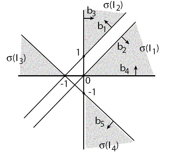
Figure 1. The hyperplane arrangement corresponding to Example 4.7

The expansion of $F(z)$ (cf. (4.12)) from the vertex corresponding to $z_{1}z_{2}z_{5}$ in the Newton polytope of the denominator of $F$ gives:

$$z_{1}z_{5}\,F(z) = \sum_{m\in\mathbb{N}^{2}}\frac{(m_{1}+m_{2})!}{m_{1}!\,m_{2}!}x_{1}^{m_{1}}x_{2}^{m_{2}}$$

$$= \sum_{m_{1}\geq m_{2}}\frac{(m_{1}+m_{2})!}{m_{1}!\,m_{2}!}x_{1}^{m_{1}}x_{2}^{m_{2}}\ +\sum_{m_{2}>m_{1}}\frac{(m_{1}+m_{2})!}{m_{1}!\,m_{2}!}x_{1}^{m_{1}}x_{2}^{m_{2}}$$

$$= \varphi_{\sigma(I_{1})}(x)-\varphi_{\sigma(I_{2})}(x)$$

Similarly, the series $\varphi_{\sigma(I_{3})}(x)$ and $\varphi_{\sigma(I_{4})}(x)$ correspond to the expansions from the other two vertices of the Newton polytope of the denominator of $F$.

5. Classification of codimension two gkz-rational configurations

In this section we prove Theorem 1.2 classifying all codimension-two configurations $A$ admitting stable rational $A$-hypergeometric functions. In particular we obtain a description of all gkz-rational configurations $A$ of codimension two.

Proof of Theorem 1.2.

As it has already been pointed out, it is shown in [9] that an essential Cayley configuration is gkz-rational and, therefore, admits stable rational $A$-hypergeometric functions. Moreover, it follows from [10] that codimension-two Lawrence configurations, while not being gkz-rational, nevertheless admit stable rational $A$-hypergeometric functions. Thus we need to consider the converse statement; that is, which codimension-two configurations admit stable, rational, $A$-hypergeometric functions.

Suppose then that $F(z)=P(z)/Q(z)$ is a stable, rational $A$-hypergeometric function. $P$ and $Q$ are $A$-homogeneous polynomial and consequently, the Newton polytope ${\mathcal{N}}(Q)$ of $Q$ lies in a translate of $\ker_{\mathbb{R}}A$. We choose a vertex $v_{Q}$ of ${\mathcal{N}}(Q)$ and a $\mathbb{Z}$-basis $\nu_{1},\nu_{2}$ of $M=\ker_{\mathbb{Z}}A$ such that

$${\mathcal{N}}(Q)\subset v_{Q}+\mathbb{R}_{\geq 0}\cdot\nu_{1}+\mathbb{R}_{\geq 0}\cdot\nu_{2}.$$

Define $x_{i}$ as in (4.8), $i=1,2$, and let $v_{P}$ be an exponent occurring in $P$. Then $F$ has $A$-homogeneity $A\cdot(v_{P}-v_{Q})$ and it has a power series expansion supported in a translate of the cone

$${\mathcal{C}}\ :=\ \mathbb{R}_{\geq 0}\cdot\nu_{1}+\mathbb{R}_{\geq 0}\cdot\nu_{2}.$$

The basis $\nu_{1},\nu_{2}$ gives rise to a Gale dual $B$ of $A$ as in Section 4 and we may choose $v=v_{P}-v_{Q}$ to identify $M_{\beta}\cong M$. We can dehomogenize $F$ to get a bivariate rational function $f(x_{1},x_{2})=p(x_{1},x_{2})/q(x_{1},x_{2})$ which verifies

$$F(z)\,=\,z^{v_{P}-v_{Q}}\ f(x_{1},x_{2}).$$

It follows from Theorem 4.2 that, without loss of generality,

$$f(x)=\varphi_{\sigma(I_{1})}+c_{2}\varphi_{\sigma(I_{2})}\cdots,$$

where $\sigma(I_{1}),\sigma(I_{2}),\ldots$ are minimal cells of the oriented line arrangement defined by $(B,v)$ contained in the first quadrant.

Since $F$ is stable, no derivative of $F$ vanishes and, after appropriate differentiation, we may assume that the degree $\beta$ lies in the Euler-Jacobi cone ${\mathcal{E}}$ and, consequently, that there are no bounded minimal cells of degree $\beta$. We can also suppose that $\sigma(I_{1})$ is a two-dimensional pointed cone with integral vertex, which we may assume to be the origin.

For each $\delta=(\delta_{1},\delta_{2})\in\sigma(I_{1})$ with $\gcd(\delta_{1},\delta_{2})=1$, the $\delta$-diagonal $f_{\delta}(t)$ of $f$ is algebraic. On the other hand, $f_{\delta}(t)=(\varphi_{\sigma(I_{1})})_{\delta}(t)$ and therefore, it follows from (4.9) that:

(5.1) $$f_{\delta}(t)=\pm\,\sum_{r\geq 0}\ \frac{\prod_{i\in I}(-\langle b_{i},\delta\rangle\,r-v_{i}-1)!}{\prod_{j\not\in I}(\langle b_{j},\delta\rangle\,r)!}\ ((-1)^{c}t)^{r}\,,$$

where $c=\langle\sum_{i\in I}b_{i},\delta\rangle$. Now, according to Theorem 2.2, for all $\delta\in\sigma(I_{1})$, the series

(5.2) $$g_{\delta}(t)=\sum_{r\geq 0}\ \frac{\prod_{i\in I}(-\langle b_{i},\delta\rangle\,r)!}{\prod_{j\not\in I}(\langle b_{j},\delta\rangle\,r)!}\ t^{r}\,$$

is an algebraic function. We note that, after cancellation, the coefficients of the series (5.2) no longer involve terms coming from pairs $b_{i}$, $b_{j}$ such that $b_{i}=-b_{j}$. We denote by $\tilde{B}\subset\mathbb{R}^{2}$ the configuration obtained by removing all such pairs as well as any zero vector and call it the reduced configuration of $B$.

If $\tilde{B}=\emptyset$ then $A$ is clearly a Lawrence configuration. Next we show that if $A$ admits a stable, rational hypergeometric function then $\tilde{B}$ cannot be a one-dimensional vector configuration.

Indeed, suppose $\tilde{B}$ is one dimensional, say, $\tilde{B}\subseteq\langle\gamma\rangle\subseteq\mathbb{Z}^{2}$. Since $f$ is stable, the Newton polytope ${\mathcal{N}}(q)$ is a two-dimensional polytope. Let $\nu$ be one of its vertices and let $\mu_{1}$, $\mu_{2}$ be the adjacent edges. We may assume without loss of generality that, say, $\mu_{1}$ is not orthogonal to $\gamma$. Consequently, it follows from Lemma 3.1 that the expansion of $f$ from the vertex $\nu$ contains infinitely many non-zero terms whose exponents lie in a ray with direction vector $\mu_{1}$. The restriction $u$ of $f(x)$ to such a ray is the specialization of a suitable derivative of $f$ and hence a one-variable rational function. On the other hand, $u$ is as in the hypothesis of Theorem 2.2 with the $p_{i}$’s and $q_{i}$’s of the form $\langle b,\mu_{1}\rangle$ for some $b\in\tilde{B}$. By (ii) of the Theorem these must cancel out in pairs but then since $\tilde{B}$ is one-dimensional, $\tilde{B}=\emptyset$ which is a contradiction.

Let

$$B_{1}:=\left(\begin{array}[]{rr}1&1\\ -1&0\\ 0&-1\\ \end{array}\right)\qquad B_{2}:=\left(\begin{array}[]{rr}2&0\\ 0&2\\ -1&0\\ 0&-1\\ -1&-1\\ \end{array}\right)\qquad B_{3}:=\left(\begin{array}[]{rr}2&2\\ 0&1\\ -1&-1\\ -1&0\\ 0&-2\\ \end{array}\right)\,.$$

By construction of $\tilde{B}$ there exists infinitely many $\delta\in\mathbb{N}^{2}$ with relatively prime entries such that $\tilde{B}\delta$ has no zero coordinate and no two distinct coordinates adding up to zero. For such a $\delta$ there is no cancellation of the factorials in the coefficients when we take the $\delta$-diagonal of $f$. Therefore, since $\tilde{B}$ has rank two, by the classification of algebraic hypergeometric series in one variable (see §2), there exists two pairs of linearly independent vectors $\delta,\delta^{\prime}\in\mathbb{N}^{2}$ and $\nu,\nu^{\prime}\in\mathbb{N}^{2}$ such that $\tilde{B}\delta=B_{i}\nu$ and $\tilde{B}\delta^{\prime}=B_{i}\nu^{\prime}$ for some $i=1,2,3$. In other words, there exists $U\in\operatorname{GL}_{2}(\mathbb{Q})$ such that

$$\tilde{B}=B_{i}U,$$

for some $i$. In fact, since $B_{i}$ is primitive, $U\in\mathbb{Z}^{2\times 2}$.

Now with the notation of the previous paragraph $f$ restricted to the rays $\mu_{1}$ and $\mu_{2}$ is rational. By inspection we see that if $i=2,3$ there are no two vectors in $\mathbb{Z}^{2}$ which give restrictions compatible with Theorem 2.2 (ii). (i.e., such that the coordinates of $\tilde{B}\mu_{i}$ are of the form $(0,a,-a,b,-b)^{t}$ for some $a,b\in\mathbb{N}$ up to permutation.) Therefore $i=1$ and it is now easy to check that necessarily $A$ is affinely equivalent to an essential Cayley configuration. This concludes the proof of Theorem 1.2. ∎

Remark 5.1.

The simplest series with associated matrix $B_{2}$

$$u_{2}(x,y):=\sum_{m,n\geq 0}\frac{(2m)!(2n)!}{m!n!(m+n)!}\,x^{m}y^{n}$$

was considered by Catalan. It is an algebraic function, in fact,

$$u_{2}(x,y)=\frac{1}{x+y-4xy}\left(\frac{x}{\sqrt{1-4x}}+\frac{y}{\sqrt{1-4y}}\right)$$

(see [19] for an appearance of this series in combinatorics).

Similarly, the series

$$u_{3}(x,y):=\sum_{m,n\geq 0}\frac{(2m+2n)!n!}{m!(2n)!(m+n)!}\,x^{m}y^{n}$$

with associated matrix $B_{3}$ is algebraic, in fact,

$$u_{3}(x,y)=\frac{1}{x+4y-xy}\left(\frac{x}{\sqrt{1-4x}}+\frac{y}{1-y}\right).$$

(The quickest way to prove these identities is to use a recursion for the coefficients. For $u_{2}$ for example

$$4A(m+1,n+1)=A(m+1,n)+A(m,n+1),$$

where $A(m,n):=(2m)!(2n)!/((m+n)!m!n!)$, and $u_{2}(t,0)=u_{2}(0,t)=1/\sqrt{1-4t}$.)

Note that in addition both $u_{2}$ and $u_{3}$ satisfy that all of their $\delta$-diagonals are algebraic. This is not the typical case for two variable algebraic functions.

For $B_{1}$ the natural series is

$$u_{1}(x,y):=\sum_{m,n\geq 0}\frac{(m+n)!}{m!n!}\,x^{m}y^{n}$$

which is of course rational $u_{1}(x,y)=1/(1-x-y)$.

Example 5.2.

In [9, Theorem 4.1] it was necessary to show that a bivariate series of the form:

(5.3) $$f(x_{1},x_{2})=\sum_{m\in\mathbb{N}^{2}}\frac{(p(m_{1}+m_{2})+k_{1})!(q(m_{1}+m_{2})+k_{2})!}{(m_{1}p)!(m_{1}q)!(m_{2}p)!(m_{2}q)!}\,x_{1}^{m}x_{2}^{n}\,,$$

where $p,q$ are relatively prime positive integers and $k_{1},k_{2}\in\mathbb{N}$, does not define a rational function. While the proof presented in [9] is incomplete, the result is clearly an immediate consequence of Theorem 1.2. Indeed, the $(1,1)$ univariate diagonal series

$$\sum_{m\geq 0}\frac{(2pm+k_{1})!(2qm+k_{2})!}{(pm)!^{2}(qm)!^{2}}\,z^{m}$$

should be algebraic but, then by Theorem 2.2, so should the central series

$$\ \sum_{m,n\geq 0}\frac{(2pm)!(2qm)!}{(mp)!^{2}(mq)!^{2}}\,z^{m}.$$

However, this is impossible by [25, Theorem 1] since the height of the series is $2$. We should point out that the argument in [9] was based on a correct proof for a similar case due to Laura Matusevich. The gap appears in adapting that proof to the series (5.3).

6. Toric residues and hypergeometric functions

The purpose of this section is to describe all stable $A$-hypergeometric functions in the case of codimension-two configurations. By Theorem 1.2 we may assume that $A$ is either a Lawrence configuration or an essential Cayley configuration. The first case has been studied, for arbitrary codimension, in [10]. In particular, if $A$ is a codimension-two Lawrence configuration then $A$ is a Cayley configuration of $r+2$ two-point configurations in $\mathbb{Z}^{r}$ and it follows from [10, Theorem 1.1] that the dimension of the space of stable $A$-hypergeometric functions is $r+1$ and that they may be represented by appropriate multidimensional residues. We refer the reader to [10] for details.

Thus, we will restrict ourselves to the case of essential Cayley configurations. We begin by recalling the construction of rational hypergeometric functions associated with any essential Cayley configuration by means of multivariate toric residues (we refer to [6, 7, 9, 10, 11] for details and proofs) and will then show in Theorem 6.1 that, in the codimension-two case, a suitable derivative of any stable rational hypergeometric function must be a toric residue. In particular, if $\beta\in{\mathcal{E}}$, the dimension of the space of rational $A$-hypergeometric functions is equal to $1$.

Let

$$A\,\,\,=\,\,\,\{e_{1}\}\!\times A_{1}\!\,\,\cup\,\,\cdots\,\,\cup\,\,\{e_{r+1}\}\!\times\!A_{r+1}\,\,\subset\,\,\mathbb{Z}^{r+1}\times\mathbb{Z}^{r}$$

be an essential Cayley configuration. For each $A_{i}\subset\mathbb{Z}^{r}$ consider the generic Laurent polynomial $f_{i}$ supported in $A_{i}$, that is:

$$f_{i}(t)\ =\ \sum_{\alpha\in A_{i}}\ u_{i\alpha}t^{\alpha}\ ;\quad t=(t_{1},\dots,t_{r}).$$

We set $D_{i}=\{t\in(\mathbb{C}^{*})^{r}:f_{i}(t)=0\}$. Generically on the coefficients $u_{i\alpha}$, given any $i=1,\dots,r+1$, the $r$-fold intersection

$$V_{i}\ :=\ D_{1}\cap\cdots\cap\widehat{D_{i}}\cap\cdots\cap D_{r+1}$$

is finite and, given any Laurent monomial $t^{a}$, $a\in\mathbb{Z}^{r}$, we can consider the global residue:

(6.1) $$R_{i}(a) := \sum_{\xi\in V_{i}}\,{\rm Res}_{\xi}\left(\frac{t^{a}/f_{i}}{f_{1}\cdots\widehat{f_{i}}\cdots f_{r+1}}\,\frac{dt_{1}}{t_{1}}\wedge\cdots\wedge\frac{dt_{r}}{t_{r}}\right)$$

(6.2) $$= \frac{1}{(2\pi i)^{r}}\int_{\Gamma}\frac{t^{a}}{f_{1}\cdots f_{r+1}}\,\frac{dt_{1}}{t_{1}}\wedge\cdots\wedge\frac{dt_{r}}{t_{r}}\,,$$

where ${\rm Res}_{\xi}$ denotes the local Grothendieck residue (see [21, 32]) and $\Gamma$ is an appropriate real $r$-cycle on the torus $(\mathbb{C}^{*})^{r}$.

It is shown in [6, Theorem 4.12] that if $a$ lies in the interior of the Minkowski sum of the convex hulls of $A_{1},\dots,A_{r+1}$ then the expression $(-1)^{i}R_{i}(a)$ is independent of $i$. Its common value is the toric residue $R(a)$ studied in [11, 6].

It is often useful to consider the expression obtained by replacing in (6.1) the polynomial $f_{j}$ by $f_{j}^{c_{j}}$, where $c_{j}$ is a positive integer. This change defines a function $R_{i}(c,a),c\in\mathbb{Z}_{>0}^{r+1}$, and if $a$ lies in the interior of the Minkowski sum of the convex hulls of $c_{1}\,A_{1},\dots,c_{r+1}\,A_{r+1}$ then the expression $(-1)^{i}R_{i}(c,a)$ is independent of $i$.

The toric residue $R(c,a)$ is a rational function on the coefficients $u_{i\alpha}$ and is $A$-hypergeometric of degree $\beta=(-c,-a)\in\mathbb{Z}^{r+1}\times Z^{r}$. This may be seen, for example, by differentiating under the integral sign in the expression (6.2). We refer to [7, Theorem 7] for details.

It follows from the arguments in [9, §5], that the function $R(c,a)$ does not vanish and, since for a given $c\in\mathbb{Z}^{r+1}_{>0}$, a point $a\in\mathbb{Z}^{r}$ is in the interior of the Minkowski sum of $c_{1}\,A_{1},\dots,c_{r+1}\,A_{r+1}$ if and only if $(-c,-a)$ lies in the Euler-Jacobi cone ${\mathcal{E}}$ (4.10), it follows that $R(c,a)$ is a stable rational $A$-hypergeometric function in this case.

We note that

(6.3) $$\frac{\partial R(c,a)}{\partial u_{i\alpha}}=-c_{i}\,R(c+e_{i},a+\alpha),$$

where $e_{i}$ denotes the $i$-th vector in the standard basis of $\mathbb{Z}^{r+1}$.

The family of Laurent polynomials $f_{1},\dots,f_{r+1}$ associated with a codimension-two Cayley essential configuration must consist of $r$ binomials and one trinomial. Thus, after relabeling the coefficients and an affine transformation of the exponents we may assume that

$$f_{i}\quad= z_{2i-1}\,+\,z_{2i}\cdot t_{1}^{\gamma_{i}}\ ;\qquad i=1,\dots,r$$

$$f_{r+1}\quad= z_{2r+1}\,+\,z_{2r+2}\cdot t^{\alpha_{1}}\,+\,z_{2r+3}\cdot t^{\alpha_{2}},$$

with $\gamma_{1},\dots,\gamma_{r},\alpha_{1},\alpha_{2}\in\mathbb{Z}^{r}\backslash\{0\}$.

Theorem 6.1.

Let $A\subset\mathbb{Z}^{2r+1}$ be a codimension-two Cayley essential configuration and suppose $\beta=(-c,-a)\in{\mathcal{E}}\cap\mathbb{Z}^{2}$. Then, any rational $A$-hypergeometric function of degree $\beta$ is a multiple of $R(c,a)$.

Proof.

The Gale dual $B$ of a codimension-two Cayley essential configuration is a collection of $2r+3$ vectors $b_{1},\dots,b_{2r+3}\in\mathbb{Z}^{2}$ which, after renumbering, may be assumed to be of the form:

$$b_{1}+b_{2}\ =\ \dots\ =\ b_{2r-1}+b_{2r}\ =\ b_{2r+1}+b_{2r+2}+b_{2r+3}\ =\ 0,$$

where the vectors $b_{2r+1},b_{2r+2},b_{2r+3}$ are not collinear.

As in (4.6) we denote by $\ell_{i}(x)=\langle b_{i},x\rangle+v_{i}$ the linear functionals in $\mathbb{R}^{2}$ defined by $B$ and a choice of $v\in\mathbb{Z}^{2r+3}$ such that $A\cdot v=\beta$. For $1\leq i<j\leq 3$, we set

(6.4) $$\Lambda_{ij}\,:=\,\{x\in\mathbb{R}^{2}:\ell_{2r+i}(x)\geq 0,\ \ell_{2r+j}(x)\geq 0\}.$$

Let $F(z)=P(z)/Q(z)$ be any non-zero (and hence, stable) $A$-hypergeometric function of degree $\beta$ and write $z^{-v}\cdot F(z)=f(x)=p(x)/q(x)$, where $x=(x_{1},x_{2})$ is as in (4.8).

We claim that the Newton polytope ${\mathcal{N}}(q)$ of the polynomial $q(x)$ is a triangle whose inward pointing normals are the vectors $b_{2r+1}$, $b_{2r+2}$, $b_{2r+3}$ (this is indeed the case for the residue $R(c,a)$ since its denominator is a power of the discriminant $D_{A}$, whose Newton polytope is such a triangle by [13]). Let $\nu_{0}$ be a vertex of ${\mathcal{N}}(q)$ and $\nu_{1},\nu_{2}$ the adjacent vertices. Set $\mu_{i}=\nu_{i}-\nu_{0}$, $i=1,2$. The Laurent expansion of $f(x)$ from the vertex $\nu_{0}$ is supported in a cone of the form

$${\mathcal{C}}=c_{0}+\mathbb{R}_{\geq 0}\cdot\mu_{1}+\mathbb{R}_{\geq 0}\cdot\mu_{2}\ ;\quad c_{0}\in\mathbb{Z}^{2}\,.$$

On the other hand, since $f(x)$ is the dehomogenization of an $A$-hypergeometric function, it follows from Theorem 4.2 that $f$ may be written as

(6.5) $$f\,=\,\sum_{\sigma}\alpha_{\sigma}\,\varphi_{\sigma}\,,$$

where $\sigma$ runs over all minimal regions of the hyperplane arrangement defined by the linear functionals $\ell_{i}(x)$ which are contained in the cone ${\mathcal{C}}$, and $\alpha_{\sigma}\in\mathbb{C}$.

Let $\sigma$ be any region appearing in (6.5) with a non-zero coefficient. Since $\sigma$ is minimal region, all linear forms $\ell_{i}$ have a constant sign in its interior. As noted in Remark 4.5, $\sigma$ must have a two-dimensional recession cone. Let $\delta$ be a rational direction in the interior of $\sigma$ and consider the $\delta$-diagonal of $\varphi_{\sigma}$. By Proposition 3.2, the function $(\varphi_{\sigma})_{\delta}(t)$ must be algebraic. As the series $\varphi_{\sigma}$ has the form (6.6) below, it follows from the discussion in Section 2 that this can only happen if two of the linear forms $\ell_{2r+j},j=1,2,3$, are positive (and the third one negative) over the interior of $\sigma$. This proves that $\sigma$ is contained in one of the regions $\Lambda_{ij}$.

Now, it follows from Lemma 3.1 that there must be minimal regions $\sigma_{1},\sigma_{2}\subset{\mathcal{C}}$, not necessarily distinct, appearing with non-zero coefficients in the expansion (6.5) such that $\sigma_{i}$ contains all points of the form $c_{i}+k\mu_{i}$, $i=1,2$, for suitable $c_{1},c_{2}\in\mathbb{Z}^{2}$ and $k\in\mathbb{Z}_{>0}$ sufficiently large.

Consider the series $\varphi_{\sigma_{1}}(x)$ associated to the minimal region $\sigma_{1}$. It follows from (4.5) that

(6.6) $$\varphi_{\sigma_{1}}(x)=\sum_{m\in\sigma_{1}}h(m)\frac{\prod_{\ell_{2r+j}(m)<0}(-\ell_{2r+j}(m)-1)!}{\prod_{\ell_{2r+j}(m)>0}\ell_{2r+j}(m)!}x^{m},$$

where $h(m)$ is a polynomial. But, since $f$ is a rational function we deduce that the univariate function

$$\sum_{k>>0}h(c_{1}+k\mu_{1})\frac{\prod_{\langle b_{2r+j},\mu_{1}\rangle<0}(-\langle b_{2r+j},\mu_{1}\rangle\,k-\langle b_{2r+j},c_{1}\rangle-1)!}{\prod_{{\langle b_{2r+j},\mu_{1}\rangle>0}}(\langle b_{2r+j},\mu_{1}\rangle\,k+\langle b_{2r+j},c_{1}\rangle)!}t^{k}$$

must be a rational function. But by item ii) in Theorem 2.2 this is only possible if

$$\langle b_{2r+j},\mu_{1}\rangle=0$$

for some $j=1,2,3$. As the ray with direction $\mu_{1}$ is in the boundary of the minimal region $\sigma_{1}$, this implies that $\sigma_{1}$ cannot be contained in $\Lambda_{ik}$, where $i,k\not=j$. Consequently, $b_{2r+j}$ is an inward pointing normal to ${\mathcal{N}}(q)$ and our claim is proved.

Given now any rational hypergeometric function $F=P/Q$ of degree $\beta$ we may now consider the Laurent expansion of its dehomogenization $f=p/q$ from the vertex of ${\mathcal{N}}(q)$ defined by the edges with inward-pointing normals $b_{2r+1}$ and $b_{2r+2}$. When that expansion is written as in (6.5) there must be, by Lemma 3.1, a minimal region $\sigma$ whose recession cone has a boundary line orthogonal to $b_{2r+1}$ and the corresponding coefficient $a_{\sigma}$ must be non-zero. Hence, the map $F\mapsto a_{\sigma}$ is $1:1$ and the space of rational $A$-hypergeometric functions of degree $\beta$ has dimension at most one. As we have already recalled, it follows from [9, §5] that the toric residue $R(c,a)$ is a non zero rational $A$-hypergeometric function of degree $\beta$, which thus spans the vector space of all rational $A$-hypergeometric functions of this degree. ∎

Example 6.2.

We continue with Example 4.7. Let $F(z)$ be as in (4.12) and $f_{1},f_{2}\in\mathbb{C}[t]$ as in (4.13). Then we have

$$F(z)\,=\,-R(1)\,=\,-{\rm Res}_{-z_{1}/z_{2}}\left(\frac{dt/f_{2}(t)}{f_{1}(t)}\right).$$

We showed in Example 4.7 that in inhomogeneous coordinates

$$z_{1}z_{5}\,F(z)\,=\,\varphi_{\sigma(I_{1})}(x)-\varphi_{\sigma(I_{2})}(x)$$

for the minimal regions $\sigma(I_{1}),\sigma(I_{2})$ contained in the first quadrant. According to Theorem 6.1 neither $\varphi_{\sigma(I_{1})}(x)$ nor $\varphi_{\sigma(I_{2})}(x)$ can be rational functions. Indeed, one can check by direct computation that, up to sign, $\varphi_{\sigma(I_{1})}(x)$ and $\varphi_{\sigma(I_{2})}(x)$ agree with the pointwise residues:

$${\rm Res}_{\xi_{\pm}}\left(\frac{dt/f_{1}(t)}{f_{2}(t)}\right),$$

where $\xi_{\pm}$ are the roots of $f_{2}(t)$:

$$\xi_{\pm}\,:=\,\frac{-z_{5}\pm\sqrt{z_{5}^{2}-4z_{3}z_{4}}}{2z_{4}}$$

and, in the inhomogeneous coordinates $x_{1}$, $x_{2}$, we have:

$$\varphi_{\sigma(I_{1})}(x) = \sum_{m_{1}\geq m_{2}\geq 0}\frac{(m_{1}+m_{2})!}{m_{1}!\,m_{2}!}\ x_{1}^{m_{1}}x_{2}^{m_{2}}$$

$$= \frac{1}{2(1-x_{1}-x_{2})}\left(1+\frac{1-2x_{2}}{\sqrt{1-4x_{1}x_{2}}}\right)\,.$$

7. Classical bivariate rational hypergeometric series

In this section we will apply the previous results to study the rationality of power series in two variables which generalize the univariate series discussed in Section 2, that is, series whose coefficients are ratios of products of factorials of linear forms defined over $\mathbb{Z}$.

Our starting data will be a support cone ${\mathcal{C}}$ which will be assumed to be a two-dimensional rational, convex polyhedral cone in $\mathbb{R}^{2}$ and linear functionals

(7.1) $$\ell_{i}(x)\,:=\,\langle b_{i},x\rangle+k_{i}\,,\quad i=1,\dots,n,$$

where $b_{i}\in\mathbb{Z}^{2}\backslash\{0\}$, $k_{i}\in\mathbb{Z}$. We will denote by $\mu_{1},\mu_{2}$ the primitive integral vectors defining the edges of ${\mathcal{C}}$ and by $\nu_{1},\nu_{2}\in\mathbb{Z}^{2}$ the corresponding primitive inward normals.

Definition 7.1.

Given ${\mathcal{C}}$ and $\ell_{i}$, $i=1,\dots,n$ as above, the bivariate series:

(7.2) $$\sum_{m\in{\mathcal{C}}\cap\mathbb{Z}^{2}}\frac{\prod_{\ell_{i}(m)<0}\ (-1)^{\ell_{i}(m)}\,(-\ell_{i}(m)-1)!}{\prod_{\ell_{j}(m)>0}\ \ell_{j}(m)!}\,x_{1}^{m_{1}}x_{2}^{m_{2}}.$$

will be called a Horn series.

Remark 7.2.

Let $\phi(x_{1},x_{2})=\sum_{m\in{\mathcal{C}}\cap\mathbb{Z}^{2}}c_{m}x^{m}$ be a Horn series as in (7.2). Then, the coefficients $c_{m}$ satisfy a Horn recurrence; that is, for $j=1,2$, and any $m\in{\mathcal{C}}\cap\mathbb{Z}^{2}$ such that $m+e_{j}$ also lies in ${\mathcal{C}}$, the ratios:

$$R_{j}(m)\,:=\,\frac{c_{m+e_{j}}}{c_{m}}\,=\,\frac{\prod_{b_{ij}<0}\prod_{l=0}^{-b_{ij}+1}\ell_{i}(m)-l}{\prod_{b_{ij}>0}\prod_{l=1}^{b_{ij}}\ell_{i}(m)+l}.$$

are rational functions of $m$ (recall that $e_{j}$ denote the standard basis vectors).

We are interested in studying when a Horn series defines a rational function $\phi(x_{1},x_{2})$. We will assume that

(7.3) $$\sum_{i=1}^{n}b_{i}\ =\ 0\,,$$

and note that (7.3) implies that (7.2) converges for $|x^{\mu_{1}}|<\varepsilon$, $|x^{\mu_{2}}|<\varepsilon$ for any small $\varepsilon>0$.

Remark 7.3.

Every Horn series (7.1) is the dehomogenization of an $A$-hypergeometric function for some regular configuration $A$. More precisely, there exists a codimension-two configuration $A\subset Z^{s-2}$, a vector $v\in\mathbb{Z}^{s}$, a $\mathbb{Z}$-basis $\nu_{1},\nu_{2}$ of $\ker_{\mathbb{Z}}(A)$, and an $A$-hypergeometric function $F(z)$ of degree $A\cdot v$ such that:

$$F(z_{1},\dots,z_{s})\,=\,z^{v}\ \phi(z^{\nu_{1}},z^{\nu_{2}})\,.$$

This may be seen as follows: the linear forms $\ell_{1},\dots,\ell_{n}$ define an oriented hyperplane arrangement associated with the vector configuration

$$B\,=\,\{b_{1},\dots,b_{n}\}$$

and the vector $(k_{1},\dots,k_{n})$. We can enlarge $B$ to a new configuration $\hat{B}$ by adding to $B$ pairs of vectors $\{c,-c\}$ where $c$ ranges over all $b_{i}\in B$, $\nu_{1},\nu_{2}$, and the standard basis vectors $e_{1}$, $e_{2}$. $\hat{B}$ is the Gale dual of a configuration $A$ and, for a suitable choice of parameter $\hat{v}\in\mathbb{Z}^{s}$, $s=|\hat{B}|$, every region in the hyperplane arrangement defined by $(\hat{B},\hat{v})$ is minimal. and the series (7.2) is the dehomogenization of an $A$-hypergeometric series of degree $A\cdot\hat{v}$.

The following theorem characterizes rational bivariate Horn series:

Theorem 7.4.

Let $\ell_{i}(x)=\langle b_{i},x\rangle+k_{i}$, $i=1,\dots,n$, be linear forms on $\mathbb{R}^{2}$ defined over $\mathbb{Z}$ and ${\mathcal{C}}$ a two-dimensional rational, convex, polyhedral cone in $\mathbb{R}^{2}$. Let

$$\phi(x_{1},x_{2})=\sum_{m\in{\mathcal{C}}\cap\mathbb{Z}^{2}}\frac{\prod_{\ell_{i}(m)<0}\ (-1)^{\ell_{i}(m)}\,(-\ell_{i}(m)-1)!}{\prod_{\ell_{j}(m)>0}\ \ell_{j}(m)!}\,x_{1}^{m_{1}}x_{2}^{m_{2}}.$$

be a Horn series satisfying (7.3). Set $B=\{b_{1},\dots,b_{n}\}\subset\mathbb{Z}^{2}$. If $\phi(x_{1},x_{2})$ is a rational function then either

• $n=2r$ is even and, after reordering we may assume:

  (7.4) $$b_{1}+b_{r+1}=\cdots=b_{r}+b_{2r}=0,\ or$$

• $B$ consists of $n=2r+3$ vectors and, after reordering, we may assume that $b_{1},\dots,b_{2r}$ satisfy (7.4) and $b_{2r+1}=s_{1}\nu_{1}$, $b_{2r+2}=s_{2}\nu_{2}$, $b_{2r+3}=-b_{2r+1}-b_{2r+2}$, where $\nu_{1},\nu_{2}$ are the primitive, integral, inward-pointing normals of ${\mathcal{C}}$ and $s_{1},s_{2}$ are positive integers.

Proof.

As noted in Remark 7.3, the series $\phi(x_{1},x_{2})$ may be viewed as the dehomogenization of an $A$-hypergeometric function, for a suitable regular configuration $A$ whose Gale dual $\hat{B}$ is obtained from $B$ by adding pairs of vectors $\{c,-c\}$, $c\in\mathbb{Z}^{2}$. Since $A$ admits a stable rational hypergeometric function, it follows from Theorem 1.2 that $A$ is either a Lawrence configuration or a Cayley essential configuration. It is now clear that in the first case, $B$ satisfies (7.4), while in the second, $n=2r+3$ and we may assume that $b_{1},\dots,b_{2r}$ also satisfy (7.4), while

$$b_{2r+1}+b_{2r+2}+b_{2r+3}=0$$

Moreover, if $A$ is a Cayley essential configuration then it is shown in the proof of Theorem 6.1 that

$$\phi(x)\,=\,\sum a_{\sigma}\varphi_{\sigma}(x),$$

where $\varphi_{\sigma}(x)$ are canonical series, as in (4.9), associated with the minimal regions of the hyperplane arrangement of $\hat{B}$, and the sum runs over all minimal regions contained in one of the sectors defined by the half-spaces $\ell_{2r+1}\geq 0$, $\ell_{2r+2}\geq 0$, $\ell_{2r+3}\geq 0$. But then, since the expansion (7.2) is not supported in any proper subcone of ${\mathcal{C}}$, it follows that ${\mathcal{C}}$ must agree with one of those sectors. Hence, after reordering if necessary, we have that

$$b_{2r+1}=s_{1}\nu_{1},\quad b_{2r+2}=s_{2}\nu_{2}.$$

∎

Example 7.5.

As an illustration of the type of series Theorem 7.4 refers to consider the following expansion from [20][Example 9.2]

$$\varphi(x)=\frac{1-x_{1}x_{2}}{1-x_{1}x_{2}^{2}-3x_{1}x_{2}-x_{1}^{2}x_{2}}=\sum_{m\in{\mathcal{C}}\cap\mathbb{Z}^{2}}\binom{m_{1}+m_{2}}{2m_{1}-m_{2}}\,x_{1}^{m_{1}}x_{2}^{m_{2}},$$

where ${\mathcal{C}}:=\{2m_{1}-m_{2}\geq 0,2m_{2}-m_{1}\geq 0\}$.

The series

(7.5) $$\phi(x)=\varphi(-x)=\sum_{m\in{\mathcal{C}}\cap\mathbb{Z}^{2}}(-1)^{m_{1}+m_{2}}\binom{m_{1}+m_{2}}{2m_{1}-m_{2}}\,x_{1}^{m_{1}}x_{2}^{m_{2}}$$

is a Horn series. It follows from Theorem 6.1 that $\phi(x)$ may be represented as a residue. Indeed, following the notation of Theorem 7.4, the configuration $B$ is defined by the vectors $b_{1}=(-1,-1)$, $b_{2}=(-1,2)$, $b_{3}=(2,-1)$. We enlarge it to a configuration $\hat{B}$ by adding the vectors $b_{4}=(1,0)$, and $b_{5}=(-1,0)$. Now, $\hat{B}$ is the Gale dual of the Cayley essential configuration

$$A\ =\ \left(\begin{array}[]{rrrrrrr}1&1&1&0&0\\ 0&0&0&1&1\\ 0&1&2&0&3\\ \end{array}\right)$$

and $\phi(x)$ is the dehomogenization of an $A$-hypergeometric toric residue associated to $f_{1}=z_{1}+z_{2}t+z_{3}t^{2},f_{2}=z_{4}+z_{5}t^{3}$. Explicitely, in inhomogeneous coordinates we have:

$$\phi(x)\,=\,\sum_{\eta}{\rm Res}_{\eta}\left(\frac{x_{2}t/(x_{2}+x_{2}t-t^{2})}{x_{2}+x_{1}t^{3}}\,dt\right),$$

where $\eta$ runs over the three cubic roots of $-x_{2}/x_{1}$; that is, $\phi$ is the global residue with respect to the family of polynomials $x_{2}+x_{1}t^{3}$ of the rational function of $t$ (depending parametrically on $x$) defined by $t/(1+t-x_{2}^{-1}t^{2})$.

In the remainder of this section we consider the special case where ${\mathcal{C}}$ is the first quadrant. The following series will play a central role in our discussion.

Proposition 7.6.

The series

(7.6) $$f_{(s_{1},s_{2})}(x)\,:=\,\sum_{m\in\mathbb{N}^{2}}\frac{(s_{1}m_{1}+s_{2}m_{2})!}{(s_{1}m_{1})!(s_{2}m_{2})!}\ x_{1}^{m_{1}}x_{2}^{m_{2}}\,.$$

defines a rational function for all $(s_{1},s_{2})\in\mathbb{N}^{2}$.

Proof.

The assertion is evident if either $s_{1}=0$ or $s_{2}=0$ since in this case (7.6) becomes:

(7.7) $$f_{0}(x_{1},x_{2})\ =\ \sum_{m\in\mathbb{N}^{2}}x_{1}^{m_{1}}x_{2}^{m_{2}}\ =\ \frac{1}{(1-x_{1})(1-x_{2})}\,,$$

as well as in the case when $s_{1}=s_{2}=1$ since

$$f_{(1,1)}(x)\,=\,\,\sum_{m\in\mathbb{N}^{2}}\frac{(m_{1}+m_{2})!}{m_{1}!\,m_{2}!}\ x_{1}^{m_{1}}x_{2}^{m_{2}}\,=\,\frac{1}{1-x_{1}-x_{2}}.$$

More in general, given any $s_{1},s_{2}>0$, consider the Cayley essential configuration:

$$A\ =\ \left(\begin{array}[]{rrrrrrr}1&1&1&0&0&0&0\\ 0&0&0&1&1&0&0\\ 0&0&0&0&0&1&1\\ 1&0&0&0&s_{1}&0&0\\ 0&1&0&0&0&0&s_{2}\\ \end{array}\right)$$

and $\beta=(-1,-1,-1,-s_{1},-s_{2})^{t}=A\cdot(0,0,-1,0,-1,0,-1)^{t}$. Consider the hyperplane arrangement associated with the vector $(0,0,-1,0,-1,0,-1)^{t}$ and the Gale dual $B$ of $A$ with rows $b_{1}=(s_{1},0),b_{2}=(0,s_{2}),b_{3}=(-s_{1},-s_{2})$, $b_{4}=(1,0)=-b_{5}$, $b_{6}=(0,1)=-b_{7}$. The first quadrant is a minimal region and the corresponding Laurent $A$-hypergeometric series is:

$$F(z)\ =\ \frac{1}{z_{3}z_{5}z_{7}}\sum_{m\in\mathbb{N}^{2}}\frac{(s_{1}m_{1}+s_{2}m_{2})!}{(s_{1}m_{1})!(s_{2}m_{2})!}\left(\frac{(-z_{1})^{s_{1}}z_{4}}{z_{3}^{s_{1}}z_{5}}\right)^{m_{1}}\left(\frac{(-z_{2})^{s_{2}}z_{6}}{z_{3}^{s_{2}}z_{7}}\right)^{m_{2}}.$$

Thus, the rationality $F$ implies that of $f_{(s_{1},s_{2})}$. But, since the first quadrant is the only minimal region contained in the open half space $\{s_{1}m_{1}+s_{2}m_{2}\geq 0\}$ and $A$ is a Cayley essential configuration, the series $F(z)$ must agree with a Laurent expansion of the toric residue

$${\rm Res}\left(\frac{t_{1}^{s_{1}}t_{2}^{s_{2}}/(z_{1}t_{1}+z_{2}t_{2}+z_{3})}{(z_{4}+z_{5}t_{1}^{s_{1}})(z_{6}+z_{7}t_{2}^{s_{2}})}\,\frac{dt_{1}}{t_{1}}\wedge\frac{dt_{2}}{t_{2}}\right),$$

which is a rational function. In fact, we can write explicitly:

(7.8) $$f_{(s_{1},s_{2})}(x)\,=\,\sum_{\xi_{1}^{s_{1}}=-x_{1},\xi_{2}^{s_{2}}=-x_{2}}{\rm Res}_{\xi}\left(\frac{t_{1}^{s_{1}}t_{2}^{s_{2}}/(t_{1}+t_{2}+1)}{(x_{1}+t_{1}^{s_{1}})(x_{2}+t_{2}^{s_{2}})}\,\frac{dt_{1}}{t_{1}}\wedge\frac{dt_{2}}{t_{2}}\right).$$

∎

An alternative proof of Proposition 7.6 follows from the the fact that $f_{(1,1)}$ is rational together with the following two lemmas, which are of independent interest.

Lemma 7.7.

Suppose

$$\sum_{m\in\mathbb{N}^{2}}a(m_{1},m_{2})\,x_{1}^{r_{1}m_{1}}x_{2}^{r_{2}m_{2}},$$

for some fixed positive integers $r_{1},r_{2}$, is the Taylor expansion of a rational function $f(x_{1},x_{2})$. Then the same is true of

$$\sum_{m\in\mathbb{N}^{2}}a(m_{1},m_{2})\,x_{1}^{m_{1}}x_{2}^{m_{2}}.$$

Proof.

Write $f=A/B$, where $A,B$ are relatively prime polynomials in $\mathbb{C}[x_{1},x_{2}]$. For any $\zeta_{1},\zeta_{2}\in\mathbb{C}^{2}$ such that $\zeta_{1}^{r_{1}}=\zeta_{2}^{r_{2}}=1$ we have

$$A(\zeta_{1}x_{1},\zeta_{2}x_{2})\,B(x_{1},x_{2})=A(x_{1},x_{2})\,B(\zeta_{1}x_{1},\zeta_{2}x_{2}).$$

Hence

$$A(\zeta_{1}x_{1},\zeta_{2}x_{2})=c\,A(x_{1},x_{2}),\qquad B(\zeta_{1}x_{1},\zeta_{2}x_{2})=c\,B(x_{1},x_{2})$$

for some non-zero constant $c\in\mathbb{C}$. Since $B(0,0)$ is nonzero (as we assume $f$ is holomorphic at the origin) evaluating at $(0,0)$ shows $c=1$ and the result follows. ∎

Lemma 7.8.

Suppose

$$\sum_{m\in\mathbb{N}^{2}}a(m_{1},m_{2})\,x_{1}^{m_{1}}x_{2}^{m_{2}}$$

is the Taylor expansion of a rational function $f(x_{1},x_{2})$. Then the same is true of

$$\sum_{m\in\mathbb{N}^{2}}a(r_{1}m_{1},r_{2}m_{2})\,x_{1}^{m_{1}}x_{2}^{m_{2}},$$

for any fixed $(r_{1},r_{2})\in\mathbb{Z}_{>0}^{2}$.

Proof.

Note that

(7.9) $$\sum_{m\in\mathbb{N}^{2}}a(r_{1}m_{1},r_{2}m_{2})\,x_{1}^{r_{1}m_{1}}x_{2}^{r_{2}m_{2}}=\frac{1}{r_{1}r_{2}}\sum_{\zeta_{1}^{r_{1}}=\zeta_{2}^{r_{2}}=1}f(\zeta_{1}x_{1},\zeta_{2}x_{2}),$$

for sufficiently small $|x_{1}|$ and $|x_{2}|$. The right hand side is clearly a rational function. Hence our claim follows from Lemma 7.7. ∎

Note that the local sum of residues  (7.8) has the same form as the sum in (7.9) in the proof of Lemma 7.8.

Example 7.9.

Consider the case $s=(2,2)$. By definition

$$f_{(2,2)}(x_{1},x_{2})=\sum_{m\in\mathbb{N}^{2}}\frac{(2m_{1}+2m_{2})!}{(2m_{1})!(2m_{2})!}\,x_{1}^{m_{1}}x_{2}^{m_{2}}.$$

Equality (7.9) reads

$$f_{(2,2)}(x_{1}^{2},x_{2}^{2})=\tfrac{1}{4}(f(x_{1},x_{2})+f(-x_{1},x_{2})+f(x_{1},-x_{2})+f(-x_{1},-x_{2})),$$

where $f(x):=f_{(1,1)}(x)$. Then,

$$f_{(2,2)}(x_{1}^{2},x_{2}^{2})\,=\,\frac{1-x_{1}^{2}-x_{2}^{2}}{1-2x_{1}^{2}-2x_{2}^{2}-2x_{1}^{2}x_{2}^{2}+x_{1}^{4}+x_{2}^{4}},$$

and hence

$$f_{(2,2)}(x_{1},x_{2})=\frac{1-x_{1}-x_{2}}{1-2x_{1}-2x_{2}-2x_{1}x_{2}+x_{1}^{2}+x_{2}^{2}}.$$

Our last result shows that, up to the action of differential operators of the form 7.10 below, all rational Horn series with support on all the integer points of the first quadrant are given by the functions $f_{(s_{1},s_{2})}$.

Theorem 7.10.

Let $\ell_{i}(x)=\langle b_{i},x\rangle+k_{i}$, $i=1,\dots,n$, be linear forms on $\mathbb{R}^{2}$ defined over $\mathbb{Z}$ and suppose that the Horn series

$$\phi(x_{1},x_{2})=\sum_{m\in\mathbb{N}^{2}}\frac{\prod_{\ell_{i}(m)<0}\ (-1)^{\ell_{i}(m)}\,(-\ell_{i}(m)-1)!}{\prod_{\ell_{j}(m)>0}\ \ell_{j}(m)!}\,x_{1}^{m_{1}}x_{2}^{m_{2}}.$$

satisfies (7.3) and defines a rational function.

Then, there exist differential operators $P_{1}(\theta),P_{2}(\theta)$ of the form

(7.10) $$\prod_{j}\langle b_{j},\theta\rangle+c_{j},\quad\theta=(\theta_{1},\theta_{2}),\,\theta_{i}=x_{i}\,\partial/\partial x_{i}\,;\ c_{j}\in\mathbb{Z},$$

such that

$$P_{1}(\theta)\cdot\phi(x)\,=\,P_{2}(\theta)\cdot f_{(s_{1},s_{2})}(\pm x_{1},{\pm}x_{2}),$$

where $s_{1}=s_{2}=0$ in case $B=\{b_{1},\dots,b_{n}\}$ is a Lawrence configuration and $s_{1},s_{2}>0$ if $B$ is Cayley essential.

Proof.

It follows from Theorem 7.4 that $B$ must be either a Lawrence or a Cayley essential configuration. In the latter case, we have moreover that $n=2r+3$, $b_{1},\dots,b_{2r}$ are as in (7.4) while $b_{2r+1}=(s_{1},0)$, $b_{2r+2}=(0,s_{2})$, $b_{2r+3}=(-s_{1},-s_{2})$ for $s_{1},s_{2}$ positive integers. Therefore, we can find a differential operator $P_{1}(\theta)$ as in (7.10) such that

$$P_{1}(\theta)\cdot\phi(x)=\pm\sum_{m\in\mathbb{N}^{2}}\left(\prod_{i=1}^{r}\prod_{j=c_{i}}^{d_{i}}(\langle b_{i},m\rangle+j)\right)\frac{(s_{1}m_{1}+s_{2}m_{2}+k)!}{(s_{1}m_{1})!(s_{2}m_{2})!}(\pm x_{1})^{m_{1}}(\pm x_{2})^{m_{2}},$$

for suitable integers $c_{i},d_{i}$. Thus taking

$$P_{2}(\theta)\,=\,\pm\left(\prod_{i=1}^{r}\prod_{j=c_{i}}^{d_{i}}(\langle b_{i},\theta\rangle+j)\right)\,\prod_{j=1}^{k}(s_{1}\theta_{1}+s_{2}\theta_{2}+j),$$

we get

$$P_{1}(\theta)(\phi(x))=P_{2}(\theta)(f_{(s_{1},s_{2})}(\pm x_{1},\pm x_{2})).$$

The argument in the Lawrence case is completely analogous. ∎

Example 7.11.

We return to the rational function in Example 7.5:

$$\phi(x)\,=\,\frac{1-x_{1}x_{2}}{1+x_{1}x_{2}^{2}-3x_{1}x_{2}+x_{1}^{2}x_{2}},$$

and its Laurent expansion (7.5). Let $m_{1}^{\prime}=2m_{1}-m_{2},m_{2}^{\prime}=2m_{2}-m_{1}$ (so that $m_{1}=\frac{2m_{1}^{\prime}+m_{2}^{\prime}}{3},m_{2}=\frac{m_{1}^{\prime}+2m_{2}^{\prime}}{3}$) then

$$\phi(x)\,=\,\sum_{{{(m_{1}^{\prime},m_{2}^{\prime})\in L\cap\mathbb{N}^{2}}}}\frac{(m_{1}^{\prime}+m_{2}^{\prime})!}{m_{1}^{\prime}!m_{2}^{\prime}!}\ u_{1}^{m_{1}^{\prime}}u_{2}^{m_{2}^{\prime}},$$

where $L$ denotes the sublattice $L=\mathbb{Z}(1,2)+\mathbb{Z}(2,1)=\{(m_{1}^{\prime},m_{2}^{\prime})\in\mathbb{Z}^{2}:m_{1}^{\prime}\equiv m_{2}^{\prime}\bmod 3\}$ and ${{u_{1}^{3}=x^{2}y,u_{2}^{3}=xy^{2}}}$. Thus, we get an expansion similar to that of $f_{(1,1)}$ but the sum is only over the points in the first quadrant that lie in the sublattice $L$ of index $3$ rather than all of $\mathbb{N}^{2}$.

References

• [1] J. Bell and J. Bober, Bounded step functions and factorial ratio sequences. Preprint: arXiv:0710.3459v1.
• [2] F. Beukers Algebraic A-hypergeometric Functions arXiv:0812.1134v1
• [3] F. Beukers and G. Heckman, Monodromy for the hypergeometric function ${}_{n}F_{n-1}$. Invent. Math., 95(2): 325–354, 1989.
• [4] J. Bober, Factorial ratios, hypergeometric series, and a family of step functions, J. London Math. Soc. To appear, 2009.
• [5] A. Borisov, Quotient singularities, integer ratios of factorials, and the Riemann Hypothesis. International Mathematics Research Notices , rnn052, 2008.
• [6] E. Cattani, D. Cox, and A. Dickenstein, Residues in toric varieties. Compositio Mathematica  108 (1997) 35–76.
• [7] E. Cattani and A. Dickenstein, A global view of residues in the torus. Journal of Pure and Applied Algebra  117 & 118 (1997) 119–144.
• [8] E. Cattani and A. Dickenstein, Balanced Configurations of Lattice Vectors and GKZ-rational Toric Fourfolds in ${\mathbb{P}}^{6}$. Journal of Algebraic Combinatorics, 19: 47–65, 2004.
• [9] E. Cattani, A. Dickenstein, and B. Sturmfels, Rational hypergeometric functions. Compositio Math., 128: 217–240, 2001.
• [10] E. Cattani, A. Dickenstein, and B. Sturmfels, Binomial Residues. Annales Institut Fourier., 52, (2002), 687–708.
• [11] D. Cox, Toric residues. Arkiv för Matematik  34 (1996) 73–96.
• [12] P. Deligne, Intégration sur un cycle évanescent Invent. Math 76 (1984) 129–143.
• [13] A. Dickenstein and B. Sturmfels, Elimination theory in codimension 2. J. Symbolic Comput., 34(2):119–135, 2002.
• [14] B. Dwork and A. van der Poorten, The Eisenstein constant, Duke Math. J. 65 (1992), no. 1, 23–43; Duke Math. J. 76 (1994), no. 2, 669–672.
• [15] H. Furstenberg, Algebraic functions over finite fields. Journal of Algebra 7 (1967), 271–277.
• [16] I. M. Gel’fand, A. Zelevinsky, and M. Kapranov, Hypergeometric functions and toral manifolds, Functional Analysis and its Appl. 23 (1989) 94–106.
• [17] I. M. Gel’fand, M. Kapranov, and A. Zelevinsky, Generalized Euler integrals and ${\mathcal{A}}$-hypergeometric functions, Advances in Math. 84 (1990) 255–271.
• [18] I. M. Gelfand, M. M. Kapranov, and A. V. Zelevinsky, Discriminants, Resultants, and Multidimensional Determinants. Birkhäuser, 1994.
• [19] I. Gessel Super ballot numbers J. Symbolic Comput. 14 (1992), no. 2-3, 179–194.
• [20] I. Gessel and G. Xin, The generating function of ternary trees and continued fractions. Electron. J. Combin. 13 (2006), no. 1, Research Paper 53, 48 pp. (electronic).
• [21] P. Griffiths and J. Harris. Principles of algebraic geometry. Pure and Applied Mathematics. Wiley-Interscience, New York, 1978.
• [22] A. H. M. Levelt, Hypergeometric functions. Doctoral thesis, University of Amsterdam. Drukkerij Holland N. V., Amsterdam, 1961.
• [23] M. Passare, T. Sadykov, and A. Tsikh, Singularities of hypergeometric functions in several variables. Compos. Math. 141:3 (2005), 787?-810.
• [24] G. Polya, Sur les seéries entières, dont la somme est une fonction algébrique. L’Enseignement mathématique 22 (1922), 38–47.
• [25] F. Rodríguez Villegas, Integral ratios of factorials and algebraic hypergeometric functions. Preprint: arXiv:math.NT/0701362.
• [26] F. Rodríguez Villegas, Hypergeometric families of Calabi-Yau manifolds, Calabi-Yau varieties and mirror symmetry (Toronto, ON, 2001), 223–231, Fields Inst. Commun., 38, Amer. Math. Soc., Providence, RI, 2003.
• [27] F. Rodríguez Villegas, Experimental Number Theory. Oxford Graduate Texts in Mathematics 13. Oxford University Press, 2007.
• [28] K. V. Safonov, On power series of algebraic and rational functions in $\mathbb{C}^{n}$. Journal of Mathematical Analysis and Applications 243 (2000), 261–277.
• [29] M. Saito, B. Sturmfels, and N. Takayama, Hypergeometric polynomials and integer programming. Compositio Math. 155 (1999), 185–204.
• [30] M. Saito, B. Sturmfels, and N. Takayama, Gröbner Deformations of Hypergeometric Differential Equations. Springer-Verlag, Berlin, 2000.
• [31] B. Sturmfels, On the Newton polytope of the resultant. J. Algebraic Combin. 3 (1994), 207–236.
• [32] A. Tsikh, Multidimensional Residues and Their Applications, American Math. Society, Providence, 1992.
• [33] V. I. Vasyunin, On a system of step functions, Zap. Nauchn. Sem. S.-Peterburg. Otdel. Mat. Inst. Steklov. (POMI) 262 (1999), no. Issled. po Linein. Oper. i Teor. Funkts. 27, 49–70, 231–232, Translation in J. Math. Sci.(New York) 110 (2002), no. 5, 2930–2943.