Filling in the Gaps in the 4.85 GHz Sky

Stephen E. Healey¹¹affiliation: Department of Physics/KIPAC, Stanford University, Stanford, CA 94305, USA ⁶⁶affiliation: Email: sehealey@astro.stanford.edu , Lars Fuhrmann²²affiliation: Max-Planck-Institut für Radioastronomie, Bonn, Germany , Gregory B. Taylor³³affiliation: Department of Physics and Astronomy, University of New Mexico, Albuquerque, NM 87131, USA ⁵⁵affiliation: G. B. Taylor is also an Adjunct Astronomer at the National Radio Astronomy Observatory. ,
Roger W. Romani¹¹affiliation: Department of Physics/KIPAC, Stanford University, Stanford, CA 94305, USA , Anthony C. S. Readhead⁴⁴affiliation: Department of Astronomy, California Institute of Technology, Pasadena, CA 91125, USA

Abstract

We describe a 4.85 GHz survey of bright, flat-spectrum radio sources conducted with the Effelsberg 100 m telescope in an attempt to improve the completeness of existing surveys, such as CRATES. We report the results of these observations and of follow-up 8.4 GHz observations with the VLA of a subset of the sample. We comment on the connection to the WMAP point source catalog and on the survey’s effectiveness at supplementing the CRATES sky coverage.

galaxies: active — quasars: general — radio continuum: galaxies — surveys

1 Introduction

Extensive effort has been made to survey the sky at 4.85 GHz with single-dish telescopes. The Parkes-MIT-NRAO survey (PMN; Griffith & Wright 1993), conducted with the 64 m telescope at Parkes, covers the region $-87\arcdeg<\delta<+10\arcdeg$ to a flux density limit of $\sim$ 30 mJy. The Green Bank 6 cm survey (GB6; Gregory et al. 1996), conducted with the former 91 m telescope at Green Bank, covers the region $0\arcdeg<\delta<+75\arcdeg$ to a limit of $\sim$ 18 mJy. The Fifth 5 GHz Strong Source Survey (S5; Kühr et al. 1981), conducted with the Effelsberg 100 m telescope, covers the region $+70\arcdeg<\delta<+90\arcdeg$ to a limit of $\sim$ 250 mJy. Together, they constitute a (non-uniform) catalog of almost 125,000 distinct radio sources over nearly the entire sky.

Data from these surveys were subsequently used to select targets for more specialized study. The Cosmic Lens All-Sky Survey (CLASS; Myers et al. 2003; Browne et al. 2003) identified sources that were bright in GB6 and had flat spectra between the 1.4 GHz NRAO VLA Sky Survey (NVSS; Condon et al. 1998) and GB6; these were then observed at 8.4 GHz with the VLA to look for gravitationally lensed compact radio sources. Although the objective of CLASS was to find lenses, Sowards-Emmerd et al. (2003) demonstrated its usefulness in identifying $\gamma$ -ray blazars, which correlate strongly with bright, flat-spectrum radio sources. The Combined Radio All-sky Targeted Eight GHz Survey (CRATES; Healey et al. 2007) extended the CLASS procedure to the entire sky with the explicit goal of identifying blazar candidates. It used the full complement of 4.85 GHz sources to identify over 11,000 bright sources with flat spectra, which were followed up with 8.4 GHz interferometry.

Much of the utility of the CRATES sample, especially with regard to identifying blazar candidates, is in its breadth of coverage and its uniformity. Sowards-Emmerd et al., for example, developed a figure of merit for associating radio sources with $\gamma$ -ray detections. The ability to do so in a statistically meaningful way rested on the uniform selection criteria and large area coverage of CLASS. Similarly, the Candidate Gamma-Ray Blazar Survey (CGRaBS; Healey et al. 2008) is a catalog of the $\sim$ 15% of CRATES sources that are most similar to the Third EGRET Catalogue (3EG; Hartman et al. 1999) blazars as quantified by a radio/X-ray figure of merit. Without the large number of consistently selected sources provided by CRATES, a catalog with the statistical power of CGRaBS would be impossible to compile. Improving the sample’s coverage is further motivated by comparison with other all-sky surveys, such as the Wilkinson Microwave Anisotropy Probe (WMAP ) five-year point source catalog (Wright et al., 2008). This shallow but uniform high-frequency radio survey of the entire sky is composed mostly of bright, flat-spectrum sources; thus, the identification of low-frequency counterparts depends on the availability of all-sky low-frequency data.

It is therefore of some importance to note that the sky coverage of the large 4.85 GHz surveys—S5, GB6, and PMN—is not perfect. In the north polar cap (an area of $\sim$ 700 square degrees), the S5 survey is considerably shallower than GB6 and PMN, as noted above. There are also two “holes” in the PMN survey just south of the equator (an area of $\sim$ 300 square degrees) in which no data are available at all. These holes are already known to contain $\gamma$ -ray blazars in 3EG and in the list of bright AGNs (Abdo et al., 2009) detected in the first three months of data from the Large Area Telescope (LAT) on board the Fermi Gamma-ray Space Telescope. Likewise, it is expected that $\gamma$ -ray blazars not associated with S5 sources will also be detected by the LAT in the far north. The real solution to this problem is a full 4.85 GHz survey of the entire northern cap and PMN hole regions down to the CRATES flux density limit ( $\sim$ 65 mJy) or better; such a campaign would require approximately a week of observing time. However, in the interest of time and logistics, we have conducted a targeted 4.85 GHz survey, requiring only $\sim$ 24 hours of observing time, of selected sources in these regions with the Effelsberg 100 m telescope as an initial step toward filling in the gaps in the CRATES all-sky coverage.

2 Sample Selection

2.1 Sky Regions

Our work concerns two distinct regions on the sky. The “north polar cap” is the region $+75\arcdeg<\delta<+90\arcdeg$ , spanning all right ascensions. The “PMN holes” are two nearly parallelogram-shaped regions just south of the equator. Their vertices, given as $(\alpha,\delta)$ in decimal degrees (J2000 coordinates), are approximately as follows:

PMN hole 1: $(175\arcdeg,0\arcdeg)$ ; $(183\arcdeg,0\arcdeg)$ ; $(197\arcdeg,-9.5\arcdeg)$ ; $(188\arcdeg,-9.5\arcdeg)$ .
PMN hole 2: $(195\arcdeg,0\arcdeg)$ ; $(217\arcdeg,0\arcdeg)$ ; $(235\arcdeg,-9.5\arcdeg)$ ; $(210\arcdeg,-9.5\arcdeg)$ .

2.2 Choosing Sources

Our goal was to observe flat-spectrum targets that were likely to be bright at 4.85 GHz. In order to select such sources, we drew from archival radio surveys at lower frequencies. NVSS provides 1.4 GHz coverage of the entire $\delta>-40\arcdeg$ sky, but to identify sources with flat spectra, data at a second frequency are required. In the north polar cap, 325 MHz data are available from the Westerbork Northern Sky Survey (WENSS; Rengelink et al. 1997) while in the PMN holes, 365 MHz data are available from the Texas Survey (Douglas et al., 1996). We identified NVSS sources with counterparts in WENSS/Texas and computed the spectral index of each source (assuming a power law spectrum $S\propto\nu^{\alpha}$ ). From this, we calculated a predicted 4.85 GHz flux density ( $S_{\mathrm{pred}}$ ) for each source. Due to logistical considerations at Effelsberg, the final selection criteria were slightly different for the two observing regions. In the north polar cap, we selected sources with $S_{\mathrm{pred}}>65$ mJy and $\alpha>-0.6$ that were not already included in the S5 survey (221 sources). It is worth noting that S5 itself only contains 236 sources, so our observations nearly double the coverage in this region. In the equatorial holes, we selected sources with $S_{\mathrm{pred}}>75$ mJy and $\alpha>-1.0$ (174 sources).

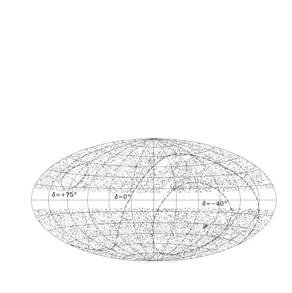
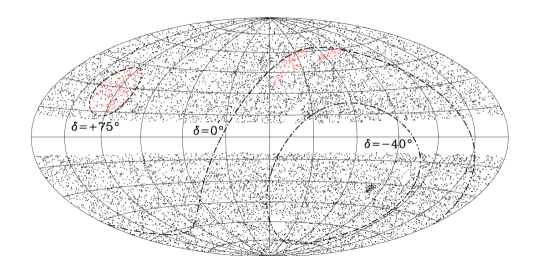
The top panel of Figure 1 shows a sky map of the sources in the CRATES catalog. The bottom panel shows the the additional sources selected for observation at Effelsberg.

3 Observations and Data Analysis

The flux density measurements of the selected sources were performed with the Effelsberg 100 m telescope of the Max-Planck-Institut für Radioastronomie (MPIfR) during two observing runs in June and July 2008 with a total observing time of $\sim$ 24 hrs. We used the 4.85 GHz multi-horn receiver permanently mounted at the secondary focus for sensitive continuum measurements. The 4.85 GHz system is a double-horn heterodyne receiver that allows the subtraction of the off-source atmospheric contribution from the on-source astronomical signal. Both circular polarizations are fed into a broad-band polarimeter, measuring the total power (Stokes I).

The target sources are sufficiently bright in the observed frequency band to allow flux density measurements using cross-scans in azimuth and elevation. In contrast to the on-off observing technique, this enables an instantaneous control of the telescope pointing as well as the identification of possible problems with confused or extended sources. Sources with $S_{\mathrm{pred}}\geq 100$ mJy were observed with four cross-scans (two in each direction), and sources with $S_{\mathrm{pred}}<100$ mJy were observed with six cross-scans (three in each direction).

In order to minimize slewing time, we observed sources along stripes parallel to the right ascension axis and about $3\arcdeg$ wide in declination. In the case of particularly weak sources (or obviously bad scans), sources were subsequently re-observed to improve S/N. We observed primary flux density calibrators (e.g., 3C 286, 3C 295 and NGC 7027) frequently to adjust the focus of the telescope and to link the measured flux densities to the absolute flux density scale (Baars et al., 1977; Ott et al., 1994).

The first steps in the data reduction included baseline subtraction and fitting of a Gaussian profile to each individual sub-scan in both slewing directions: the peak of the Gaussian measures the antenna temperature on the source, the HPBW ( $\sim$ $144\arcsec$ ), and the positional displacement of the peak (i.e., the residual pointing error of the telescope, typically $<$ $10\arcsec$ ). We flagged bad scans or sub-scans and excluded them from further analysis. For sources showing confusion problems (i.e., a secondary source in the off-horn position, causing severe distortion), we reduced the data without the software beam-switch. After correcting the measured amplitudes for residual positional offsets using the approximately Gaussian shape of the telescope beam, we averaged them over both slewing directions. We performed an opacity correction using the $T_{\mathrm{sys}}$ measurements obtained for each sub-scan and a standard correction for the systematic elevation-dependent telescope gain. The frequent primary calibrator measurements allowed us to convert the measured antenna temperatures for each target into absolute flux densities.

4 Results

In total, we observed 395 sources across both sky regions. For 368 (93%) of the sources, we obtained precise flux densities with a mean fractional uncertainty of 2.3%. The individual measurement uncertainties result mostly from statistical errors in the reduction process (including errors from the Gaussian fit) and a contribution from the scatter seen in the primary calibrator measurements. By independently studying a large sample of weak sources at 4.85 GHz, Angelakis et al. (2009) showed that for flux densities $\lesssim$ 100 mJy, the dominant sources of uncertainty are thermal noise, confusion, and tropospheric instabilities. Together, they result in an uncertainty of about 1.2 mJy, which we also include in our error estimates. The 4.85 GHz flux densities and uncertainties are given in Table 1 (for the sources in the north polar cap) and Table 2 (for the sources in the PMN holes). The NVSS positions were sufficient given the pointing accuracy of the Effelsberg 100 m telescope, and they are more accurate than can be measured by the 100 m telescope, so we report the NVSS positions in the tables.

5 VLA Follow-up

We conducted a follow-up campaign on 109 sources (72 in the north polar cap and 37 in the PMN holes), with the VLA in the A configuration, using two 50 MHz bands at 8.44 GHz. We targeted sources with $S_{\mathrm{4.85\;GHz}}\geq 65$ mJy from our Effelsberg observations and $\alpha>-0.6$ between 1.4 GHz (from NVSS) and 4.85 GHz. The observations took place on 2008 November 1 as part of program AH0976, and the on-source dwell time was 60 s. Standard AIPS calibration was performed, followed by Difmap imaging and Gaussian component fitting. We used 3C 286 as a flux density calibrator, and the typical radiometric error is approximately 3%. With interferometric X-band measurements in hand, these sources are now completely on par with those in CRATES.

The results of these observations are shown in Tables 1 and 2. We report the position and integrated flux density of each source. For sources with multiple components, we report the position and integrated flux density of each individual component. The typical positional accuracy is $\lesssim$ $0.06\arcsec$ , which is consistent with the positional uncertainties of the calibrators and the expected positional accuracy under good conditions. Four sources (J0033+7829, J0202+8115, J1445 $-$ 0329, and J2329+7808) have components that were resolved by the VLA; these are less likely to be the compact cores of blazars and are indicated in the tables.

6 WMAP Point Sources

The WMAP five-year data release includes a list of 390 point sources detected in the sky maps of at least one of the WMAP frequency bands (K = 23 GHz, Ka = 33 GHz, Q = 41 GHz, V = 61 GHz, W = 94 GHz). This provides an all-sky high-frequency radio catalog of the sky against which to check our selection of bright, flat-spectrum sources. Healey et al. showed that the vast majority ( $\sim$ 88%) of sources in the WMAP three-year point source catalog (Hinshaw et al., 2006) had counterparts in CRATES. Those that did not were dominated by sources that were very bright but had steep spectra. However, some of the sources without counterparts were bright, flat-spectrum sources that were simply located in regions not covered by CRATES (e.g., the Galactic plane and the PMN holes). At the WMAP areal density ( $9.5\times 10^{-3}$ deg^-2), we expect the PMN holes to contain $\sim$ 3 WMAP sources, and indeed, two sources (WMAP J1408 $-$ 0749 and WMAP J1512 $-$ 0904) are located there and another (WMAP J1510 $-$ 0546) is right on the edge of the PMN coverage. Our sample selection included these three sources (i.e., they were not specially targeted), and our 4.85 GHz data confirm that they are indeed bright, flat-spectrum sources like those in the CRATES sample.

7 Discussion

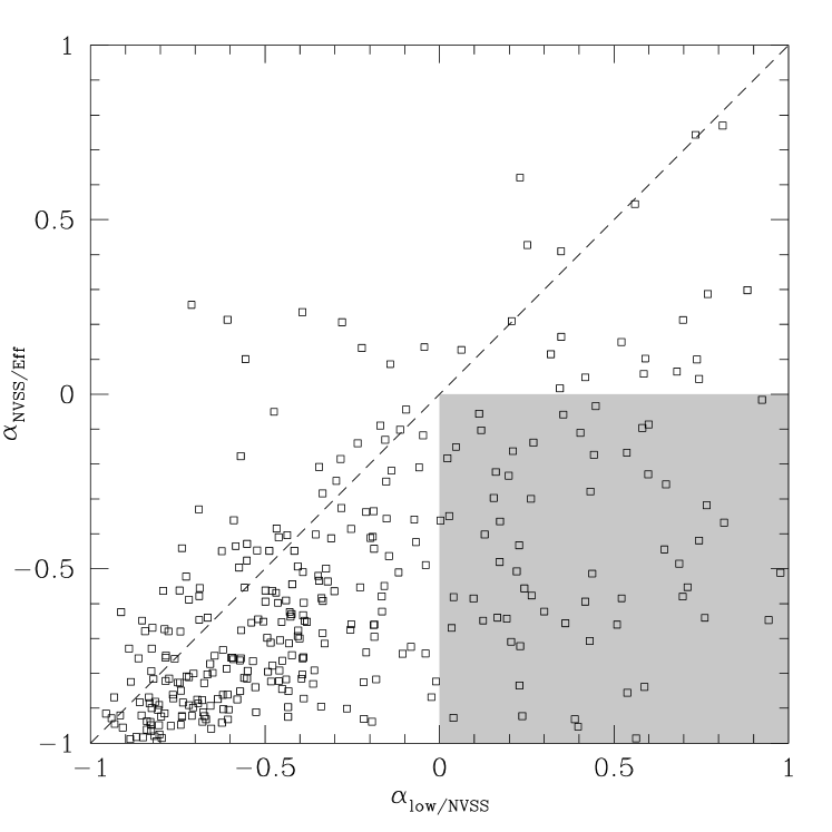
Figure 2 shows a comparison of the observed 4.85 GHz flux densities to the flux densities predicted as described in §2.2. As the distribution shows, our simple power-law extrapolation is not a very good indicator of the true flux density; it overpredicts the observed value for $\sim$ 80% of the targets, and $\langle S_{\mathrm{obs}}/S_{\mathrm{pred}}\rangle$ = 0.75. As a result, many of the observed sources do not end up satisfying the nominal CRATES cuts on flux density ( $S_{\mathrm{4.8\;GHz}}\geq 65$ mJy) and/or spectral index ( $\alpha>-0.5$ ). Indeed, by requiring a bright detection at $\sim$ 0.35 GHz, we seem to have selected a significant number of gigahertz-peaked spectrum (GPS) sources rather than strong flat-spectrum 4.85 GHz sources. Figure 3 shows a scatter plot of the spectral index between 1.4 GHz and 4.85 GHz (“ $\alpha_{\mathrm{NVSS/Eff}}$ ”) vs. the spectral index between $\sim$ 0.35 GHz and 1.4 GHz (“ $\alpha_{\mathrm{low/NVSS}}$ ”). The shaded region represents sources with spectra that rise from $\sim$ 0.35 GHz to 1.4 GHz but fall from 1.4 GHz to 4.85 GHz (i.e., GPS sources); our catalog contains 75 such sources. Note also that most sources ( $>$ 80%) fall below the dashed line, indicating spectra that are steeper above 1.4 GHz than below it. An alternative approach to sample selection, such as simply targeting the brightest NVSS sources, may have yielded a higher fraction of CRATES-like sources.

Nevertheless, the results of this survey are of value. Of the $\sim$ 160 CRATES-like sources sources missing in the north polar cap, we have identified 57, bringing the coverage there from $\sim$ 33% to $\sim$ 57%. Of the $\sim$ 100 missing sources in the PMN holes, we have identified 24, bringing the coverage there from 0% to $\sim$ 24%. The total coverage of the $|b|>10\arcdeg$ sky is increased from 97.6% to 98.3%. This catalog of strong, compact sources with subarcsecond astrometry is also of great use for calibrating radio telescope arrays. Additionally, our 4.85 GHz survey, along with the 8.4 GHz follow-up measurements, brings the fraction of high-latitude WMAP point sources with CRATES-like counterparts to 84%. Our observations will be even more important in the Planck era; the increase in sensitivity ( $\sim$ 30 $\times$ ) over WMAP will yield thousands of point sources over the entire sky, and the identification of counterparts will rely heavily on catalogs of bright, flat-spectrum radio sources.

Data in this paper are based on observations with the 100 m telescope of the MPIfR (Max-Planck-Institut für Radioastronomie) at Effelsberg. The National Radio Astronomy Observatory is operated by Associated Universities, Inc., under cooperative agreement with the National Science Foundation. S. E. H. was supported by SLAC under DOE contract DE-AC03-76SF00515.

References

Abdo et al. (2009) Abdo, A. A. et al. 2009, ApJ, 700, 597.
Angelakis et al. (2009) Angelakis, E. et al. 2009, A&A, in press; arXiv:0905.2660.
Baars et al. (1977) Baars, J. W. M., Genzel, R., Pauliny-Toth, I. I. K., & Witzel, A. 1977, A&A, 61, 99.
Browne et al. (2003) Browne, I. W. A. et al. 2003, MNRAS, 341, 13.
Condon et al. (1998) Condon, J. J., Cotton, W. D., Greisen, E. W., Yin, Q. F., Perley, R. A., Taylor, G. B., & Broderick, J. J. 1998, AJ, 115, 1693.
Douglas et al. (1996) Douglas, J. N., Bash, F. N., Bozyan, F. A., Torrence, G. W., & Wolfe, C. 1996, AJ, 111, 1945.
Gregory et al. (1996) Gregory, P. C., Scott, W. K., Douglas, K., Condon, J. J. 1996, ApJS, 103, 427.
Griffith & Wright (1993) Griffith, M. R. & Wright, A. E. 1993, AJ, 105, 1666.
Hartman et al. (1999) Hartman, R. C. et al. 1999, ApJS, 123, 79.
Healey et al. (2007) Healey, S. E., Romani, R. W., Taylor, G. B., Sadler, E. M., Ricci, R., Murphy, T., Ulvestad, J. S., & Winn, J. N. 2007, ApJS, 171, 61.
Healey et al. (2008) Healey, S. E. et al. 2008, ApJS, 175, 97.
Hinshaw et al. (2006) Hinshaw, G. et al. 2007, ApJS, 170, 288.
Kühr et al. (1981) Kühr, H., Pauliny-Toth, I. I. K., Witzel, A., & Schmidt, J. 1981, AJ, 86, 854.
Myers et al. (2003) Myers, S. T. et al. 2003, MNRAS, 341, 1.
Ott et al. (1994) Ott, M., Witzel, A., Quirrenbach, A., Krichbaum, T. P., Standke, K. J., Schalinski, C. J., & Hummel, C. A. 1994, A&A, 284, 331.
Rengelink et al. (1997) Rengelink, R. B., Tang, Y., de Bruyn, A. G., Miley, G. K., Bremer, M. N., Röttgering, H. J. A., & Bremer, M. A. R. 1997, A&AS, 124, 259.
Sowards-Emmerd et al. (2003) Sowards-Emmerd, D., Romani, R. W., & Michelson, P. F. 2003, ApJ, 590, 109.
Wright et al. (2008) Wright, E. L. et al. 2008, ApJS, 180, 283.

Table 1: Sources in the north polar cap

Name	NVSS position		$S_{4.85}$	$\sigma_{4.85}$	VLA 8.4 GHz position		$S_{8.4}$ ^a^aThe typical error in the 8.4 GHz flux density is approximately 3%.
	(J2000)		(mJy)	(mJy)	(J2000)		(mJy)
J0010 $+$ 7614	00:10:17.83	$+$ 76:14:19.8	25.4	1.2
J0022 $+$ 7501	00:22:02.13	$+$ 75:01:22.5	34.0	1.3
J0029 $+$ 8031	00:29:27.15	$+$ 80:31:31.6	80.0	1.6
J0032 $+$ 8750	00:32:41.68	$+$ 87:50:43.7	57.1	1.4
J0033 $+$ 7829	00:33:08.23	$+$ 78:29:00.8	67.4	1.5	00:33:08.211	$+$ 78:29:00.12	48.5^b^bComponent is resolved or partially resolved.
J0045 $+$ 8810	00:45:02.55	$+$ 88:10:17.9	66.6	1.5
J0054 $+$ 7558	00:54:30.73	$+$ 75:58:08.0	66.6	1.5
J0115 $+$ 8109	01:15:42.01	$+$ 81:09:54.2	52.2	1.4
J0128 $+$ 7928	01:28:08.93	$+$ 79:28:46.1	113.3	1.9	01:28:08.870	$+$ 79:28:46.14	93.0
J0138 $+$ 8611	01:38:29.65	$+$ 86:11:40.1	68.0	1.5	01:38:29.637	$+$ 86:11:40.90	38.7
J0143 $+$ 8544	01:43:35.52	$+$ 85:44:22.7	82.0	1.6	01:43:35.551	$+$ 85:44:23.50	68.4
J0144 $+$ 7958	01:44:37.08	$+$ 79:58:39.5	19.6	1.2
J0151 $+$ 8303	01:51:18.31	$+$ 83:03:20.2	51.6	1.4
J0157 $+$ 7552	01:57:11.56	$+$ 75:52:28.8	102.6	1.8
J0202 $+$ 8115	02:02:05.42	$+$ 81:15:45.0	163.7	2.4	02:02:05.739	$+$ 81:15:45.28	47.6^b^bComponent is resolved or partially resolved.
J0211 $+$ 8449	02:11:41.58	$+$ 84:49:47.7	78.4	1.6	02:11:41.338	$+$ 84:49:47.92	55.5
J0215 $+$ 7554	02:15:17.69	$+$ 75:54:53.6	96.6	1.7	02:15:17.902	$+$ 75:54:53.01	68.9
J0249 $+$ 8019	02:49:40.73	$+$ 80:19:25.3	38.6	1.3
J0249 $+$ 8435	02:49:48.43	$+$ 84:35:56.4	126.7	2.0	02:49:48.331	$+$ 84:35:57.03	121.0
J0304 $+$ 7930	03:04:56.81	$+$ 79:30:52.2	26.4	1.2
J0309 $+$ 8601	03:09:42.29	$+$ 86:01:39.7	27.0	1.3
J0316 $+$ 7720	03:16:32.19	$+$ 77:20:59.2	115.6	1.9	03:16:32.143	$+$ 77:20:58.40	133.7
J0317 $+$ 7658	03:17:51.96	$+$ 76:58:33.9	83.2	1.6	03:17:54.072	$+$ 76:58:38.06	13.4
J0320 $+$ 8711	03:20:21.87	$+$ 87:11:18.6	50.6	1.4
J0324 $+$ 7849	03:24:14.60	$+$ 78:49:10.9	106.1	1.8	03:24:14.531	$+$ 78:49:11.65	82.6
J0325 $+$ 8517	03:25:11.23	$+$ 85:17:40.0	82.9	1.6	03:25:11.125	$+$ 85:17:39.45	42.7
					03:25:13.732	$+$ 85:17:43.70	4.4
J0410 $+$ 8208	04:10:39.50	$+$ 82:08:23.3	115.3	1.9
J0411 $+$ 8509	04:11:52.15	$+$ 85:09:43.9	52.5	1.4
J0428 $+$ 7528	04:28:18.59	$+$ 75:28:00.3	18.8	1.2
J0428 $+$ 8314	04:28:21.90	$+$ 83:14:55.3	48.7	1.4
J0440 $+$ 7755	04:40:18.91	$+$ 77:55:58.5	56.3	1.4
J0442 $+$ 8742	04:42:25.51	$+$ 87:42:57.4	21.3	1.2
J0449 $+$ 8233	04:49:00.25	$+$ 82:33:18.8	197.8	2.8	04:49:00.184	$+$ 82:33:19.45	150.7
J0501 $+$ 8505	05:01:54.66	$+$ 85:05:19.9	15.3	1.2
J0517 $+$ 8108	05:17:57.65	$+$ 81:08:51.9	13.3	1.2
J0524 $+$ 7627	05:24:22.17	$+$ 76:27:35.4	58.6	1.4
J0532 $+$ 7623	05:32:29.80	$+$ 76:23:28.3	56.8	1.4
J0540 $+$ 7702	05:40:52.10	$+$ 77:02:01.5	46.8	1.3
J0546 $+$ 7943	05:46:48.52	$+$ 79:43:25.2	31.1	1.3

Note. — Only the first page of Table 1 is shown here. The table is published in its entirety in the electronic edition.

Table 2: Sources in the PMN holes

Name	NVSS position		$S_{4.85}$	$\sigma_{4.85}$	VLA 8.4 GHz position		$S_{8.4}$ ^a^aThe typical error in the 8.4 GHz flux density is approximately 3%.
	(J2000)		(mJy)	(mJy)	(J2000)		(mJy)
J1144 $-$ 0031	11:44:54.01	$-$ 00:31:36.6	215.8	3.1
J1146 $-$ 0007	11:46:40.93	$-$ 00:07:33.7	42.6	1.3
J1146 $-$ 0108	11:46:42.88	$-$ 01:08:05.1	121.8	2.0
J1148 $-$ 0046	11:48:07.19	$-$ 00:46:45.3	165.5	2.5
J1150 $-$ 0023	11:50:43.88	$-$ 00:23:54.4	1797.8	23.4
J1156 $-$ 0212	11:56:38.19	$-$ 02:12:53.8	71.8	1.5
J1157 $-$ 0124	11:57:11.03	$-$ 01:24:11.0	69.9	1.5
J1157 $-$ 0312	11:57:50.08	$-$ 03:12:23.8	148.2	2.3
J1202 $-$ 0240	12:02:32.28	$-$ 02:40:03.3	219.9	3.1
J1202 $-$ 0336	12:02:51.43	$-$ 03:36:26.6	97.5	1.7
J1204 $-$ 0029	12:04:05.69	$-$ 00:29:50.0	157.7	2.4	12:04:05.683	$-$ 00:29:53.55	50.7
J1204 $-$ 0422	12:04:02.13	$-$ 04:22:44.0	962.7	12.6
J1207 $-$ 0106	12:07:41.66	$-$ 01:06:37.4	153.5	2.3	12:07:41.679	$-$ 01:06:36.67	107.7
					12:07:42.244	$-$ 01:06:47.11	6.5
					12:07:41.589	$-$ 01:06:39.67	4.9
J1209 $-$ 0257	12:09:06.88	$-$ 02:57:45.2	106.5	1.8
J1210 $-$ 0136	12:10:31.37	$-$ 01:36:50.1	258.0	3.6
J1210 $-$ 0341	12:10:18.86	$-$ 03:41:54.0	65.4	1.5
J1213 $-$ 0159	12:13:14.00	$-$ 01:59:04.0	52.5	1.4
J1214 $-$ 0306	12:14:50.51	$-$ 03:06:49.2	86.5	1.6	12:14:50.517	$-$ 03:06:49.55	65.0
J1214 $-$ 0416	12:14:32.37	$-$ 04:16:03.4	79.6	1.6
J1214 $-$ 0606	12:14:35.91	$-$ 06:06:58.9	86.0	1.6
J1215 $-$ 0628	12:15:14.42	$-$ 06:28:03.6	308.0	4.2	12:15:14.394	$-$ 06:28:03.90	296.9
J1217 $-$ 0337	12:17:55.30	$-$ 03:37:21.2	73.3	1.5
J1218 $-$ 0631	12:18:36.18	$-$ 06:31:15.9	181.4	2.6
J1221 $-$ 0241	12:21:23.90	$-$ 02:41:50.9	448.0	5.9	12:21:23.942	$-$ 02:41:49.60	210.8
					12:21:23.921	$-$ 02:41:49.84	31.7
					12:21:30.395	$-$ 02:41:32.99	23.0
					12:21:30.409	$-$ 02:41:32.95	18.7
J1222 $-$ 0449	12:22:24.14	$-$ 04:49:33.0	62.3	1.4
J1226 $-$ 0421	12:26:46.60	$-$ 04:21:18.6	104.2	1.8
J1226 $-$ 0434	12:26:56.76	$-$ 04:34:22.2	116.1	1.9
J1227 $-$ 0445	12:27:16.53	$-$ 04:45:32.8	39.5	1.3
J1228 $-$ 0631	12:28:52.20	$-$ 06:31:46.3	191.7	2.8	12:28:52.176	$-$ 06:31:46.55	70.6
					12:28:52.192	$-$ 06:31:46.54	29.5
					12:28:52.209	$-$ 06:31:46.48	15.6
J1228 $-$ 0838	12:28:20.43	$-$ 08:38:13.1	281.7	3.9
J1230 $-$ 0510	12:30:29.00	$-$ 05:10:01.0	76.0	1.6
J1232 $-$ 0717	12:32:52.31	$-$ 07:17:29.9	172.3	2.5
J1233 $-$ 0613	12:33:31.27	$-$ 06:13:22.8	67.1	1.5

^b^bfootnotetext: Component is resolved or partially resolved.

Note. — Only the first page of Table 2 is shown here. The table is published in its entirety in the electronic edition.

Refer to caption — Figure 1: Top: Aitoff equal-area projection of the CRATES catalog in Galactic coordinates $(l,b)$ with $l=0\arcdeg$ at the center. Bottom: The same sky map with the additional Effelsberg targets shown in red.