Bayesian inference of biochemical kinetic parameters using the linear noise approximation
Abstract
Background:
Fluorescent and luminescent gene reporters allow us to dynamically quantify changes in molecular species concentration over time on the single cell level. The mathematical modeling of their interaction through multivariate dynamical models requires the development of effective statistical methods to calibrate such models against available data. Given the prevalence of stochasticity and noise in biochemical systems inference for stochastic models is of special interest. In this paper we present a simple and computationally efficient algorithm for the estimation of biochemical kinetic parameters from gene reporter data.
Results:
We use the linear noise approximation to model biochemical reactions through a stochastic dynamic model which essentially approximates a diffusion model by an ordinary differential equation model with an appropriately defined noise process. An explicit formula for the likelihood function can be derived allowing for computationally efficient parameter estimation. The proposed algorithm is embedded in a Bayesian framework and inference is performed using Markov chain Monte Carlo.
Conclusions:
The major advantage of the method is that in contrast to the more established diffusion approximation based methods the computationally costly methods of data augmentation are not necessary. Our approach also allows for unobserved variables and measurement error. The application of the method to both simulated and experimental data shows that the proposed methodology provides a useful alternative to diffusion approximation based methods.
Supplementary Information (SI):
Available at http://www.warwick.ac.uk/staff/M.Komorowski/LNASI.pdf
1 Background
The estimation of parameters in biokinetic models from experimental data is an important problem in Systems Biology. In general the aim is to calibrate the model so as to reproduce experimental results in the best possible way. The solution of this task plays a key role in interpreting experimental data in the context of dynamic mathematical models and hence in understanding the dynamics and control of complex intracellular chemical networks and the construction of synthetic regulatory circuits [1]. Among biochemical kinetic systems, the dynamics of gene expression and of gene regulatory networks are of particular interest. Recent developments of fluorescent microscopy allow us to quantify changes in protein concentration over time in single cells (e.g. [2, 3]) even with single molecule precision (see [4] for review). Therefore an abundance of data is becoming available to estimate parameters of mathematical models in many important cellular systems.
Single cell imaging techniques have revealed the stochastic nature of biochemical reactions (see [5, 6] for review) that most often occur far from thermodynamic equilibrium [7] and may involve small copy numbers of reacting macromolecules [8]. This inherent stochasticity implies that the dynamic behaviour of one cell is not exactly reproducible and that there exists stochastic heterogeneity between cells. The disparate biological systems, experimental designs and data types impose conditions on the statistical methods that should be used for inference [9, 10, 11]. From the modeling point of view the current common consensus is that the most exact stochastic description of the biochemical kinetic system is provided by the chemical master equation (CME) [12]. Unfortunately, for many tasks such as inference the CME is not a convenient mathematical tool and hence various types of approximations have been developed. The three most commonly used approximations are [13]:
-
1.
The macroscopic rate equation (MRE) approach which describes the thermodynamic limit of the system with ordinary differential equations and does not take into account random fluctuations due to the stochasticity of the reactions.
-
2.
The diffusion approximation (DA) which provides stochastic differential equation (SDE) models where the stochastic perturbation is introduced by a state dependant Gaussian noise.
-
3.
The linear noise approximation (LNA) which can be seen as a combination because it incorporates the deterministic MRE as a model of the macroscopic system and the SDEs to approximatively describe the fluctuations around the deterministic state.
Statistical methods based on the MRE have been most widely studied [14, 9, 15, 16]. They require data based on large populations. The main advantages of this method are its conceptual simplicity and the existence of extensive theory for differential equations. However, single cells experiments and studies of noise in small regulatory networks created the need for statistical tools that are capable to extract information from fluctuations in molecular species. Two methods have been proposed to address this. The one by [17] assumes availability of single molecule precision data. Another approach is based on the diffusion approximation [10, 18]. This uses likelihood approximation methods (e.g. [19]) that are computationally intensive and require sampling from high dimensional posterior distributions. Inference using these methods is particularly difficult for low frequency data with unobserved model variables [18, 11]. The aim of this study is to investigate the use of the LNA as a method for inference about kinetic parameters of stochastic biochemical systems. We find that the LNA approximation provides an explicit Gaussian likelihood for models with hidden variables and measurement error and is therefore simpler to use and computationally efficient. To account for prior information on parameters our methodology is embedded in the Bayesian paradigm. The paper is structured as follows: We first provide a description of the LNA based modeling approach and then formulate the relevant statistical framework. We then study its applicability in four examples, based on both simulated and experimental data, that clarify principles of the method.
2 Methods
The chemical master equation (CME) is the primary tool to model the stochastic behaviour of a reacting chemical system. It describes the evolution of the joint probability distribution of the number of different molecular species in a spatially homogeneous, well stirred and thermally equilibrated chemical system [12]. Even though these assumptions are not necessarily satisfied in living organisms the CME is commonly regarded as the most realistic model of biochemical reactions inside living cells. Consider a general system of chemical species inside a volume and let denote the number and the concentrations of molecules. The stoichiometry matrix describes changes in the population sizes due to different chemical events, where each describes the change in the number of molecules of type from to caused by an event of type . The probability that an event of type occurs in the time interval equals . The functions are called mesoscopic transition rates. This specification leads to a Poisson birth and death process where the probability that the system is in the state at time is described by the CME [13] which is given in the SI.
The first order terms of a Taylor expansion of the CME in powers of are given by the following MRE (see SI)
| (1) |
where and
Including also the second order terms of this
expansion produces the LNA
| (2) |
which decomposes the state of the system into a deterministic part as solution of the MRE in (1) and a stochastic process described by an Itô diffusion equation
| (3) |
where denotes increments of a Wiener process, , and (see SI for derivation).
The rationale behind the expansion in terms of is that for constant average concentrations relative fluctuations will decrease with the inverse of the square root of volume [20]. Therefore the LNA is accurate when fluctuations are sufficiently small in relation to the mean (large ). Hence, the natural measure of adequacy of the LNA is the coefficient of variation i.e. ratio of the standard deviation to the mean (see SI). Validity of this approximation is also discussed in details in [20, 21]. In addition it can be shown that the process describing the deviation from the deterministic state converges weakly to the diffusion (3) as [22]. In order to use the LNA in a likelihood based inference method we need to derive transition densities of the process .
2.1 Transition densities
The LNA provides solutions that are numerically or analytically tractable because the MRE in (1) can be solved numerically and the linear SDE in (3) for an initial condition has a solution of the form [23]
| (4) |
where the integral is in the Itô sense and is the fundamental matrix of the non-autonomous system of ODEs
| (5) |
Equations (4), (5) imply that the transition densities [24] of the process are Gaussian111Throughout the paper we use ’Gaussian’ or ’normal’ shortly to denote either a univariate or a multivariate normal distribution depending on the context.[24]
| (6) |
where denotes a vector of all model parameters, is the normal density with mean and variance specified by
| (7) | |||||
It follows from (2) and (6) that the transition densities of are normal
| (8) |
The properties of the normal distribution allow us to derive an explicit formula for the likelihood of observed data.
2.2 Inference
It is rarely possible to observe the time evolution of all molecular components participating in the system of interest [25]. Therefore, we partition the process into those components that are observed and those that are unobserved.
Let , and denote the time-series that comprise the values222Here and throughout the paper we use the same letter to denote the stochastic process and its realization. of processes , and , respectively, at times .
Our aim is to estimate the vector of unknown parameters from a sequence of measurements . Given the Markov property of the process the augmented likelihood is given by
| (9) |
where are Gaussian densities specified in (8). For mathematical convenience we assume that is also normal with mean and covariance matrix . This assumption is justified as equations (2) and (3) imply normal distribution at any time given a fixed initial condition. Mean and covariance matrix are parameterized as elements of .
It can then be shown that (see SI) is Gaussian. Therefore
| (10) |
where is Gaussian with mean vector and covariance matrix whose elements can be calculated numerically in a straightforward way (see SI). Since the marginal distributions are also Gaussian it follows that the likelihood function can be obtained from the augmented likelihood (10)
| (11) |
where the covariance matrix is a sub-matrix of such that and is the vector consisting of the observed components of .
Fluorescent reporter data are usually assumed to be proportional to the number of fluorescent molecules [26] and measurements are subject to measurement error, i.e. errors that do not influence the stochastic dynamics of the system. We therefore assume that instead of the matrix our data have the form . The parameter is a proportionality constant333It is straightforward to generalize for the case with different proportionality constants for different molecular components. and denotes a random vector for additive measurement error. For mathematical convenience we assume that the joint distribution of the measurement error is normal with mean and known covariance matrix , i.e. . If measurement errors are independent with a constant variance then . Equation (11) implies that the likelihood function can be written as
| (12) |
Since for given data the likelihood function (12) can be numerically evaluated any likelihood based inference is straightforward to implement. Using Bayes’ theorem, the posterior distribution satisfies the relation [27]
| (13) |
We use the standard Metropolis-Hastings (MH) algorithm [27] to sample from the posterior distribution in (13).
3 Results
In order to study the use of the LNA method for inference we have selected four examples which are related to commonly used quantitative experimental techniques such as measurements based on reporter gene constructs and reporter assays based on Polymerase Chain Reaction (e.g. RT-PCR, Q-PCR). For expository reasons, all case studies consider a model of single gene expression.
3.1 Model of single gene expression
Although gene expression involves various biochemical reactions it is essentially modeled in terms of only three biochemical species (DNA, mRNA, protein) and four reaction channels (transcription, mRNA degradation, translation, protein degradation) [28, 29, 30]. Let denote concentrations of mRNA and protein, respectively. The stoichiometry matrix has the form
| (14) |
where rows correspond to molecular species and columns to reaction channels. For the reaction rates
| (15) |
we can derive the following macroscopic rate equations
| (16) |
For the general case it is assumed that the transcription rate is time-dependent, reflecting changes in the regulatory environment of the gene such as the availability of transcription factors or chromatin structure.
Using (15) and (16) in (3) we obtain the following SDEs describing the deviation from the macroscopic state
| (17) | |||
We will refer to the model in (16) and (17) as the simple model of single gene expression.
In order to test our method on a nonlinear system we will also consider the case of an autregulated network where the transcription rate of the gene is a function of a modified form of the protein that the gene codes for and where the modified protein is a transcription factor that inhibits the production of its own mRNA. This is parameterized by a Hill function [28] where now describes the maximum rate of transcription, is a dissociation constant and is a Hill coefficient. Thus, the nonlinear autoregulatory model the system is described by the MRE
| (18) |
and the SDEs
| (19) |
where . We refer to this model as the autoregulatory model of single gene expression. The two models constitute the basis of our inference studies below.
3.2 Inference from fluorescent reporter gene data for the simple model of single gene expression
To test the algorithm we first use the simple model of single gene expression. We generate data according to the stoichiometry matrix (14) and rates (15) using Gillespie’s algorithm [31] and sample it at discrete time points. We then generate artificial data that are proportional to the simulated protein data with added normally distributed measurement error with known variance . Furthermore we assume that mRNA levels are unobserved. Thus the data are of the form444The volume of the system is unknown and we set so that concentration equals the number of molecules.
| (20) |
where , is the simulated protein concentration, is an unknown proportionality constant and is measurement error. For the purpose of our example we model the transcription function by
| (21) |
This form of
transcription corresponds to an experiment,
where transcription increases for as a result of being induced by an
environmental stimulus and for
decreases towards a baseline level .
We
assume that at time () the
system is in a stationary state. Therefore,
the initial condition of the MRE is a
function of unknown parameters
To ensure identifiability of all model parameters we assume that informative prior distributions for both degradation rates are available. Priors for all other parameters were specified to be non-informative.
To infer the vector of unknown parameters
we sample from the posterior distribution
using the standard MH algorithm. The distribution is given by (12).
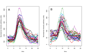
The protein level of the simulated trajectory is sampled every minutes and a sample size of points obtained. We perform inference for two simulated data sets: estimate 1 is based on a single trajectory while estimate 2 represents a larger data set using 20 sampled trajectories (see Figure 1A). All prior specifications, parameters used for the simulations and inference results are presented in Table 1A.
Estimate 1 demonstrates that it is possible to infer all parameters from a single, short length time series with a realistically achievable time resolution. Estimate 2 shows that usage of the LNA does not seem to result in any significant bias. A bias has not been detected despite the very small number of mRNA molecules (5 to 35 - Figure 2A in the SI) and protein molecules (100 to 500 - Figure 1A). The coefficient of variation varied between approximately 0.15 and 0.4 for both molecular species (Figure 1 in the SI).
Inference for this model required sampling from the 9 dimensional posterior distribution (number of unknown parameters). If instead one used a diffusion approximation based method it would be necessary to sample from a posterior distribution of much higher dimension (see SI). In addition, incorporation of the measurement error is straightforward here, whereas for other methods it involves a substantial computational cost [18].
| (A) | ||||
|---|---|---|---|---|
| Param. | Prior | Value | Estimate 1 | Estimate 2 |
| (0.44,) | 0.44 | 0.43 (0.27-0.60) | 0.49 (0.38-0.61) | |
| (0.52,) | 0.52 | 0.51 (0.35-0.67) | 0.49 (0.38-0.61) | |
| Exp(100) | 10.00 | 21.09 (3.91-67.17) | 11.41 (7.64-16.00) | |
| Exp(100) | 1.00 | 1.42 (0.60-2.57) | 1.08 (0.76-1.36) | |
| Exp(100) | 15.00 | 6.80 (0.97-18.43) | 12.78 (9.80-15.33) | |
| Exp(1) | 0.40 | 0.79 (0.05-3.02) | 0.29 (0.18-0.43) | |
| Exp(1) | 0.40 | 0.77 (0.08-2.79) | 0.77 (0.32-1.59) | |
| Exp(10) | 7.00 | 6.13 (4.41-7.85) | 7.25 (6.79-7.55) | |
| Exp(100) | 3.00 | 0.94 (0.11-2.88) | 2.87 (2.11-3.52) | |
| (B) | ||||
| Param. | Prior | Value | Estimate 1 | Estimate 2 |
| (0.44, | 0.44 | 0.44 (0.27-0.60) | 0.42 (0.32-0.54) | |
| (0.52, | 0.52 | 0.49 (0.33-0.65) | 0.49 (0.36-0.61) | |
| Exp(100) | 10.00 | 14.86 (3.18-47.97) | 9.35 (5.87-13.15) | |
| Exp(100) | 1.00 | 1.26 (0.48-2.30) | 1.15 (0.81-1.50) | |
| Exp(100) | 15.00 | 5.99 (0.20-23.06) | 13.47 (9.24-17.13) | |
| Exp(1) | 0.40 | 0.59 (0.01-2.75) | 0.27 (0.14-0.53) | |
| Exp(1) | 0.40 | 0.92 (0.05-2.92) | 0.83 (0.21-3.52) | |
| Exp(10) | 7.00 | 6.53(0.74-14.69) | 7.27 (6.44-7.79) | |
| Exp(100) | 3.00 | 2.85 (0.35-7.19) | 2.64 (1.82-3.32) |
3.3 Inference from fluorescent reporter gene data for the model of single gene expression with autoregulation
The following example considers the autoregulatory system with only a small number of reacting molecules. Using Gillespie’s algorithm we generate artificial data from the single gene expression model with autoregulation. The protein time courses were then sampled every 15 minutes at 101 discrete points per trajectory (see Figure 1B). As before we assume that the mRNA time courses are not observed and that the protein data are of the form given in (20), i.e. proportional to the actual amount of protein with additive Gaussian measurement error. As in the previous case study we estimate parameters from two simulated data sets, a single trajectory and an ensemble of 20 independent trajectories. The inference results summarized in Table 1B show that despite the low number of mRNA (0-15 molecules, see Fig. 2 in SI) and protein (10-250 molecules, see Fig. 1B) all parameters can be estimated well with appropriate precision.
3.4 Inference for PCR based reporter data
In the case of reporter assays based on Polymerase Chain Reaction (e.g. RT-PCR, Q-PCR) measurements are obtained from the extraction of the molecular contents from the inside of cells. Since the sample is sacrificed, the sequence of measurements are not strictly associated with a stochastic process describing the same evolving unit. Assume that at each time point we observe measurements that are proportional to the number of RNA molecules either from a single cell or from a population of cells. This gives a matrix of data points
| (22) |
where , is the actual RNA level, is the proportionality constant, is a Gaussian independent measurement error indexed by time ; indexes the measurements that are taken at time . Note that and are independent random variables as they refer to different cells. We assume that the dynamics of RNA is described by the simple model of single gene expression with LNA equations (16) and (17). Let denote the distribution of measured RNA at time . In order to accommodate for the different form of data we modify the estimation procedure as follows. For analytical convenience we assumed that the initial distribution is normal . This together with eq. (8) and normality of measurement error implies that . Simple explicit formulae for and are derived in the SI. Since all observations are independent we can write the posterior distribution as
| (23) |
where is the normal density with parameters . In order to infer the vector of the unknown parameters we sample from the posterior using a standard MH algorithm. To test the algorithm we have simulated a small (, , plotted in Figure 2) and a large (, ) data set using Gillespie’s algorithm with parameter values given in Table 2. The data were sampled discretely every minutes and a standard normal error was added. Initial conditions were sampled from the Poisson distribution with mean . The estimation results in Table 2 show that parameters can be inferred well in both cases even though the number of RNA molecules in the generated data is very small (about 5-35 molecules). Since subsequent measurements do not belong to the same stochastic trajectory, estimation for the model presented here is not straightforward with the diffusion approximation based methods.


| Parameter | Prior | Value | Estimate 1 | Estimate 2 |
|---|---|---|---|---|
| Exp(1) | 0.44 | 0.45 (0.35-0.60) | 0.46 (0.42-0.50) | |
| Exp(100) | 1.00 | 1.07 (0.90-1.22) | 1.01 (0.95-1.05) | |
| Exp(100) | 15.00 | 13.13 (10.20-15.87) | 14.91 (13.86-15.77) | |
| Exp(1) | 0.40 | 0.29 (0.14-0.51) | 0.43 (0.32-0.54) | |
| Exp(1) | 0.40 | 0.32 (0.12-0.93) | 0.32 (0.21-0.43) | |
| Exp(10) | 7.00 | 7.05 (6.39-7.63) | 6.99 (6.76-7.15) | |
| Exp(100) | 3.00 | 2.97 (2.00-4.18) | 3.10 (2.76-3.43) | |
| Exp(100) | 6.76 | 6.90 (5.79-7.69) | 6.55 (6.14-6.85) | |
| Exp(100) | 6.76 | 3.52 (0.01-8.99) | 7.59 (5.44-9.49) |
3.5 Estimation of gfp protein degradation rate from cycloheximide experiment
In this section the method is applied to experimental data. After a period of transcriptional induction, translation of gfp was blocked by the addition of cycloheximide (CHX). Details of the experiment are presented in the SI. Fluorescence was imaged every 6 minutes for 12.5h (see Figure 2). Since inhibition may not be fully efficient we assume that translation may be occurring at a (possibly small) positive rate . The model with the LNA is
| (24) | |||||
The observed fluorescence is assumed to be proportional to the signal with proportionality constant . For comparison we also consider the diffusion approximation for which an exact transition density can be derived analytically (see SI for derivation)
| (25) |
Since incorporation of measurement error for the diffusion approximation based model is not straightforward, we assume that measurements were taken without any error to ensure fair comparison between the two approaches. Table 3 shows that estimates obtained with both methods are very similar.
| Param. | Prior | Estimate LNA | Estimate DA |
|---|---|---|---|
| Exp(1) | 0.45 (0.31-0.62) | 0.53 (0.39-0.67) | |
| Exp(50) | 0.32(0.10-1.75) | 0.43 (0.16-1.07) | |
| Exp(50) | 22.79(13.79-36.92) | 23.85(16.31-36.54) | |
| 889.03(831.44-945.34) | - |
4 Discussion
The aim of this paper is to suggest the LNA as a useful and novel approach to the inference of biochemical kinetics parameters. Its major advantage is that an explicit formula for the likelihood can be derived even for systems with unobserved variables and data with additional measurement error. In contrast to the more established diffusion approximation based methods [10, 18] the computationally costly methods of data augmentation to approximate transition densities and to integrate out unobserved model variables are not necessary. Furthermore, this method can also accommodate measurement error in a straightforward way. The suggested procedure here is implemented in a Bayesian framework using MCMC simulation to generate posterior distributions. The LNA has previously been studied in the context of approximating Poisson birth and death processes [22, 20, 32, 21] and it was shown that for a large class of models the LNA provides an excellent approximation. Furthermore, in [32] it is shown that for the systems with linear reaction rates the first two moments of the transition densities resulting from the CME and the LNA are equal. Here we propose using the LNA directly for inference and provide evidence that the resulting method can give very good results even if the number of reacting molecules is very small. Our experience from previous works with diffusion approximation based methods [11, 18] is that their implementation is challenging especially for data that are sparsely sampled in time because the need for imputation of unobserved time points leads to a very high dimensionality of the posterior distribution. This usually results in highly autocorrelated traces affecting the speed of convergence of the Markov chain. Our method considerably reduces the dimension of the posterior distribution to the number of unknown parameters of a model only and is independent of the number of unobserved components. Nevertheless it can only be applied to the systems with sufficiently large volume, where fluctuations around a deterministic state are relatively close to the mean.
5 Authors contributions
MK proposed and implemented the algorithm. CVH performed the cycloheximide experiment. MK wrote the paper with assistance from BF and DAR, who supervised the study.
References
- [1] Ehrenberg M, Elf J, Aurell E, Sandberg R, Tegner J: Systems Biology Is Taking Off. Genome Res. 2003, 13(11):2377–2380.
- [2] Elowitz MB, Levine AJ, Siggia ED, Swain PS: Stochastic Gene Expression in a Single Cell. Science 2002, 297(5584):1183–1186.
- [3] Nelson DE, Ihekwaba AEC, Elliott M, Johnson JR, Gibney CA, et al: Oscillations in NF-kappaB Signaling Control the Dynamics of Gene Expression. Science 2004, 306(5696):704–708.
- [4] Xie SX, Choi PJ, Li GW, Lee NK, Lia G: Single-Molecule Approach to Molecular Biology in Living Bacterial Cells. Annual Review of Biophysics 2008, 37:417–444.
- [5] Raser JM, O’Shea EK: Noise in Gene Expression: Origins, Consequences, and Control. Science 2005, 309(5743):2010–2013.
- [6] Raj A, van Oudenaarden A: Nature, nurture, or chance: stochastic gene expression and its consequences. Cell 2008, 135(2):216–226.
- [7] Keizer J: Statistical Thermodynamics of Nonequilibrium Processes. Springer 1987.
- [8] Guptasarma P: Does replication-induced transcription regulate synthesis of the myriad low copy number proteins of Escherichia coli? Bioessays 1995, 17(11):987–97.
- [9] Moles CG, Mendes P, Banga JR: Parameter Estimation in Biochemical Pathways: A Comparison of Global Optimization Methods. Genome Res. 2003, 13(11):2467–2474.
- [10] Golightly A, Wilkinson DJ: Bayesian Inference for Stochastic Kinetic Models Using a Diffusion Approximation. Biometrics 2005, 61(3):781–788.
- [11] Finkenstadt B, Heron E, Komorowski M, Edwards K, Tang S, Harper C, Davis J, White M, Millar A, Rand D: Reconstruction of transcriptional dynamics from gene reporter data using differential equations. Bioinformatics 2008, 24(24):2901.
- [12] Gillespie DT: A Rigorous Derivation of the Chemical Master Equation. Physica A 1992, 188(1-3):404–425.
- [13] Van Kampen N: Stochastic Processes in Physics and Chemistry. North Holland 2006.
- [14] Mendes P, Kell D: Non-linear optimization of biochemical pathways: applications to metabolic engineering and parameter estimation. Bioinformatics 1998, 14(10):869–883.
- [15] Ramsay JO, Hooker G, Campbell D, Cao J: Parameter estimation for differential equations: a generalized smoothing approach. Journal of the Royal Statistical Society: Series B (Statistical Methodology) 2007, 69(5):741–796.
- [16] Esposito W, Floudas C: Global Optimization for the Parameter Estimation of Differential-Algebraic Systems. Industrial and Engineering Chemistry Research 2000, 39(5):1291–1310.
- [17] Reinker S, Altman R, Timmer J: Parameter estimation in stochastic biochemical reactions. Systems Biology, IEE Proceedings 2006, 153(4):168–178.
- [18] Heron EA, Finkenstadt B, Rand DA: Bayesian inference for dynamic transcriptional regulation; the Hes1 system as a case study. Bioinformatics 2007, 23(19):2596–2603.
- [19] Elerian O, Chib S, Shephard N: Likelihood Inference for Discretely Observed Nonlinear Diffusions. Econometrica 2001, 69(4):959–993.
- [20] Elf J, Ehrenberg M: Fast Evaluation of Fluctuations in Biochemical Networks With the Linear Noise Approximation. Genome Res. 2003, 13(11):2475–2484.
- [21] Ferm L, P L, Hellander A: A Hierarchy of Approximations of the Master Equation Scaled by a Size Parameter. Journal of Scientific Computing 2007, 34(2):127–151.
- [22] Kurtz TG: The Relationship between Stochastic and Deterministic Models for Chemical Reactions. The Journal of Chemical Physics 1972, 57(7):2976–2978.
- [23] Arnold L: Stochastic differential equations: theory and applications. Wiley-Interscience 1974.
- [24] Oksendal B: Stochastic differential equations (3rd ed.): an introduction with applications. Springer 1992.
- [25] Ronen M, Rosenberg R, Shraiman BI, Alon U: Assigning numbers to the arrows: Parameterizing a gene regulation network by using accurate expression kinetics. Proceedings of the National Academy of Sciences of the United States of America 2002, 99(16):10555–10560.
- [26] Wu J, Pollard TD: Counting Cytokinesis Proteins Globally and Locally in Fission Yeast. Science 2005, 310(5746):310–314.
- [27] Gamerman D, Lopes HF: Markov Chain Monte Carlo Stochastic Simulation for Bayesian Inference, 2nd ed. Chapman & Hall/CRC 2006.
- [28] Thattai M, van Oudenaarden A: Intrinsic noise in gene regulatory networks. Proceedings of the National Academy of Sciences 2001, :151588598.
- [29] Chabot JR, Pedraza JM, Luitel P, van Oudenaarden A: Stochastic gene expression out-of-steady-state in the cyanobacterial circadian clock. Nature 2007, 450:1249–1252.
- [30] Komorowski M, Miekisz J, Kierzek A: Translational Repression Contributes Greater Noise to Gene Expression than Transcriptional Repression. Biophysical Journal 2009, 96(2).
- [31] Gillespie DT: Exact stochastic simulation of coupled chemical reactions. Journal of Physical Chemistry 1977, 81(25):2340–2361.
- [32] Tomioka R, Kimurab H, Kobayashib TJ, Aihara K: Multivariate analysis of noise in genetic regulatory networks. Journal of Theoretical Biology 2004, 229(4):501–521.