Unitary equilibrations: probability distribution of the Loschmidt echo

Lorenzo Campos Venuti Institute for Scientific Interchange, Villa Gualino, Viale Settimio Severo 65, I-10133 Torino, Italy    Paolo Zanardi Department of Physics and Astronomy, and Center for Quantum Information Science & Technology, University of Southern California Los Angeles, CA 90089-0484 (USA) Institute for Scientific Interchange, Villa Gualino, Viale Settimio Severo 65, I-10133 Torino, Italy
Abstract

Closed quantum systems evolve unitarily and therefore cannot converge in a strong sense to an equilibrium state starting out from a generic pure state. Nevertheless for large system size one observes temporal typicality. Namely, for the overwhelming majority of the time instants, the statistics of observables is practically indistinguishable from an effective equilibrium one. In this paper we consider the Loschmidt echo (LE) to study this sort of unitary equilibration after a quench. We draw several conclusions on general grounds and on the basis of an exactly-solvable example of a quasi-free system. In particular we focus on the whole probability distribution of observing a given value of the LE after waiting a long time. Depending on the interplay between the initial state and the quench Hamiltonian, we find different regimes reflecting different equilibration dynamics. When the perturbation is small and the system is away from criticality the probability distribution is Gaussian. However close to criticality the distribution function approaches a double peaked, “batman-hood” shaped, universal form.

I introduction

A sudden change of the parameters governing the evolution of a closed quantum many-body system gives typically rise to a complex and fascinating dynamics. This so-called Hamiltonian quench is attracting an increasing amount of attention Calabrese and Cardy (2006); Cazalilla (2006); Manmana et al. (2007); Silva (2008). The reason for such an interest is, at least, twofold; in the first place this out of equilibrium phenomenon has been recently observed in cold atom systems Kinoshita et al. (2006); Hoffenberth et al. (2007). Secondly, at a more conceptual level, the equilibration dynamics of a quenched quantum system plays a role in the very foundations of statistical mechanics Tasaki (1998); Goldstein et al. (2006); Reimann (2007, 2008); Popescu et al. (2006); Linden et al. . New insights can be gained on the fundamental question about the emergence of a thermal behavior in closed quantum systems.

In this paper we study a prototypical dynamical quantity for a quantum quench: the Loschmidt echo (LE). This quantity is defined by the square modulus of the scalar product, of the time-evolved, (out of equilibrium) quantum state with the initial (equilibrium) one e.g., Hamiltonian ground-state.

In spite of the simplicity of its definition the Loschmidt echo \mathcal{L}, or closely related quantities, convey a great deal of information in a variety of physical problems; for example \mathcal{L} has been intensively studied in the context of Fermi edge singularities in x-ray spectra of metals Schotte and Schotte (1969), quantum chaos Prosen (1998); Jalabert and Pastawski (2001), decoherence Quan et al. (2006a); Rossini et al. (2007a, b), and more recently quantum criticality Zanardi et al. (2007) and out-of-equilibrium fluctuations Jarzynski (1997); Kurchan .

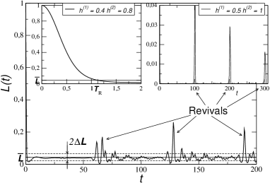
Typically (cfr. figure 1) the Loschmidt echo rapidly decays from its maximum value =11\mathcal{L}=1 at t=0𝑡0t=0 and, after an initial transient starts oscillating erraticaly around the same well defined value. For finite size systems after a sufficiently long time a pattern of collapses and revivals is observed due to the almost-periodic nature of the underlying quantum dynamics. On the other hand for infinite volume systems the Hamiltonian spectrum generically becomes continuous and an asymptotic value subscript\mathcal{L}_{\infty} (coinciding with the average one) is eventually reached.

The main goal here is to investigate the statistical properties of the Loschmidt echo seen as a random variable over the observation time interval [0,T].0𝑇[0,T]. One of the key properties is that a small variance, by standard probability theory arguments, guarantees that the overwhelming majority of the time (t)𝑡\mathcal{L}(t) sticks very close to its average value Tasaki (1998); Linden et al. ; Reimann (2008). This is the sense in which one can speak about equilibration dynamics and corresponding “equilibrium properties” of a finite system that is evolving unitarily and therefore cannot have attractive fixed points.

We shall show how the features of the probability distribution of the Loschmidt echo depend on a rich interplay between the initial state and quench Hamiltonian on the one hand and the system’s size and observation time on the other. In particular we will focus on the potential role that the vicinity of quantum critical points may have on the features of the Loschmidt echo probability distribution function Zanardi et al. (2007); Rossini et al. (2007a); Silva (2008). This latter analysis will be mostly carried over by exploiting exact results for quasi-free spin chain i.e., the quantum Ising model Zanardi et al. (2007).

The paper is organized as follows: in Section II we give the general setting. Later we introduce a relaxation time TRsubscript𝑇𝑅T_{R} and discuss the universality content of the (t)𝑡\mathcal{L}\left(t\right) before this time-scale. In Section II.3 we define and study other relevant time scales, the time T1subscript𝑇1T_{1} for necessary for observing the correct average, and revival times where large portion of (t)𝑡\mathcal{L}\left(t\right) are back in phase. In section II.4 we give explicit formulas for the moments of the LE assuming the non-resonant hypothesis. In section III we concentrate on a particular example and prove all the general results advocated so far for an exactly solvable case. Moreover we discover three universal behaviors for the whole LE probability distribution function. We draw some parallels with another natural quenched observable: the magnetization. Finally section V is devoted to conclusions and outlook.

II General Behavior

Let us start by recalling a few elementary yet crucial facts. If H=nEnΠn𝐻subscript𝑛subscript𝐸𝑛subscriptΠ𝑛H=\sum_{n}E_{n}\Pi_{n} is the system’s Hamiltonian (ΠnsubscriptΠ𝑛\Pi_{n}’s=spectral projections) the closed-system dynamics is described by the time-evolution superoperator 𝒰t=eit,(X)=[H,X].formulae-sequencesubscript𝒰𝑡superscript𝑒𝑖𝑡𝑋𝐻𝑋{\cal U}_{t}=e^{-it{\cal H}},\,{\cal H}(X)=[H,X]. This superoperator is thought here of as a map of the space of trace-class operators X𝑋X into itself (X1:=trXX<assignsubscriptnorm𝑋1trsuperscript𝑋𝑋\|X\|_{1}:={\rm{tr}}\sqrt{X^{\dagger}X}<\infty). Closed quantum systems cannot equilibrate in the strong sense, as unitary evolutions 𝒰tsubscript𝒰𝑡{\mathcal{U}}_{t} do not have non-trivial i.e., non fixed, limit points in the norm topology for t𝑡t\rightarrow\infty 111Here below we sketch why this is so. Let us suppose that ρ=limt𝒰t(ρ0).subscript𝜌subscript𝑡subscript𝒰𝑡subscript𝜌0\rho_{\infty}=\lim_{t\to\infty}{\cal U}_{t}(\rho_{0}). Obviously ρsubscript𝜌\rho_{\infty} is a fixed point for 𝒰tsubscript𝒰𝑡{\cal U}_{t} i.e., 𝒰t(ρ)=𝒰t(limu𝒰u(ρ0))=limu𝒰t+u(ρ0)=limu𝒰u(ρ0)=ρ.subscript𝒰𝑡subscript𝜌subscript𝒰𝑡subscript𝑢subscript𝒰𝑢subscript𝜌0subscript𝑢subscript𝒰𝑡𝑢subscript𝜌0subscript𝑢subscript𝒰𝑢subscript𝜌0subscript𝜌{\cal U}_{t}(\rho_{\infty})={\cal U}_{t}(\lim_{u\to\infty}{\cal U}_{u}(\rho_{0}))=\lim_{u\to\infty}{\cal U}_{t+u}(\rho_{0})=\lim_{u\to\infty}{\cal U}_{u}(\rho_{0})=\rho_{\infty}. Using unitary invariance of the trace-norm it follows that 𝒰t(ρ0)ρ1=𝒰t(ρ0ρ)1=ρ0ρ1subscriptnormsubscript𝒰𝑡subscript𝜌0subscript𝜌1subscriptnormsubscript𝒰𝑡subscript𝜌0subscript𝜌1subscriptnormsubscript𝜌0subscript𝜌1\|{\cal U}_{t}(\rho_{0})-\rho_{\infty}\|_{1}=\|{\cal U}_{t}(\rho_{0}-\rho_{\infty})\|_{1}=\|\rho_{0}-\rho_{\infty}\|_{1} and therefore limt𝒰t(ρ0)ρ1=0subscript𝑡subscriptnormsubscript𝒰𝑡subscript𝜌0subscript𝜌10\lim_{t\to\infty}\|{\cal U}_{t}(\rho_{0})-\rho_{\infty}\|_{1}=0 implies ρ0=ρ.subscript𝜌0subscript𝜌\rho_{0}=\rho_{\infty}.. One may then wonder whether a weaker form of convergence can be achieved for t𝑡t\to\infty.

Let us then consider the expectation value of an observable A(t):=tr(𝒰t(ρ0)A)assign𝐴𝑡trsubscript𝒰tsubscript𝜌0AA(t):={\rm{tr}\left({\cal U}_{t}(\rho_{0})A\right)} and write the spectral resolution of the superoperator 𝒰tsubscript𝒰𝑡{\cal U}_{t} as a formal sum 𝒰t=eit||,{\cal U}_{t}=\sum_{{\cal E}}e^{-it{\cal E}}|{\cal E}\rangle\rangle\langle\langle{\cal E}|, here {\cal E} (||{\cal E}\rangle\rangle)denote the eigenvalues (eigenvector) of .{\cal H}. In finite dimensions the kernel of {\cal H} is spanned by the ΠnsubscriptΠ𝑛\Pi_{n}’s and gives rise to a time-independent contribution to A(t)𝐴𝑡A(t) i.e., A:=ntr(Πnρ0ΠnA);assignsubscript𝐴subscript𝑛trsubscriptΠ𝑛subscript𝜌0subscriptΠ𝑛𝐴A_{\infty}:=\sum_{n}{\rm{tr}}(\Pi_{n}\rho_{0}\Pi_{n}A); the point is now to understand whether the remaining components involving the non-trivial time-dependent factors exp(it)(0)𝑖𝑡0\exp(-i{\cal E}t)\,({\cal E}\neq 0) admits a limit for t.𝑡t\rightarrow\infty. In finite dimensions the {\cal E} are a (finite) discrete set of differences of Hamiltonian eigenvalues e.g., =EnEm,subscript𝐸𝑛subscript𝐸𝑚{\cal E}=E_{n}-E_{m}, and correspondingly A(t)A𝐴𝑡subscript𝐴A(t)-A_{\infty} is a quasi-periodic function: the long time limit of A(t)𝐴𝑡A(t) does not exist. On the other hand in the infinite dimensional case the spectrum of {\cal H} can be continuous and, if the function A^():=ρ0,,Aassign^𝐴subscript𝜌0𝐴\hat{A}({\cal E}):=\langle\rho_{0},{\cal E}\rangle\langle{\cal E},A\rangle is sufficiently well behaved, using the Reimann-Lebesgue lemma, limtA^()exp(it)=0.subscript𝑡^𝐴𝑖𝑡0\lim_{t\to\infty}\hat{A}({\cal E})\exp(-i{\cal E}t)=0. Therefore in this case

limtA(t)=A(t)¯=Asubscript𝑡𝐴𝑡¯𝐴𝑡subscript𝐴\lim_{t\to\infty}A(t)=\overline{A(t)}=A_{\infty} (1)

where A(t)¯:=limT1T0TA(t)𝑑tassign¯𝐴𝑡subscript𝑇1𝑇superscriptsubscript0𝑇𝐴𝑡differential-d𝑡\overline{A(t)}:=\lim_{T\to\infty}\frac{1}{T}\int_{0}^{T}A(t)dt denotes the time-average over an infinite time interval. While this convergence cannot be achieved uniformly for the whole set of system’s observables (in that it would imply strong convergence) it can be proven for specific families of A𝐴A’s e.g., local ones Cramer et al. (2008).

There is a third form of convergence that one can consider here: the convergence in probability. In the following we shall consider the above defined A(t)𝐴𝑡A(t) as a random variable over the real line of t𝑡t endowed with the uniform measure dt/T𝑑𝑡𝑇dt/T with T.𝑇T\rightarrow\infty. Suppose we have a sequence of {BL}Lsubscriptsubscript𝐵𝐿𝐿\{B_{L}\}_{L} (think of L𝐿L as the system size), we say that the BLsubscript𝐵𝐿B_{L}’s converge to zero in probability if

limLPr{t𝐑/|BL(t)|ϵ}=0,ϵ>0.formulae-sequencesubscript𝐿Pr𝑡𝐑subscript𝐵𝐿𝑡italic-ϵ0for-allitalic-ϵ0\lim_{L\to\infty}{\rm{Pr}}\{t\in\mathbf{R}\,/\,|B_{L}(t)|\geq\epsilon\}=0,\,\forall\epsilon>0. (2)

The meaning of this type of convergence should be clear: for large L𝐿L the probability of observing a value of BL(t)subscript𝐵𝐿𝑡B_{L}(t) different from zero is vanishingly small. In other words the fractions of t𝑡t’s for which BL(t)0subscript𝐵𝐿𝑡0B_{L}(t)\neq 0 is going to zero for L.𝐿L\rightarrow\infty. As a matter of fact this is the type of convergence, with BL(t)=AL(t)AL,,subscript𝐵𝐿𝑡subscript𝐴𝐿𝑡subscript𝐴𝐿B_{L}(t)=A_{L}(t)-A_{L,\infty}, that has been considered in Reimann (2008); Linden et al. . The stochastic convergence (2) implies that the probability distributions of the random variables ALsubscript𝐴𝐿A_{L} i.e., PL(α):=δ(αAL(t))¯assignsubscript𝑃𝐿𝛼¯𝛿𝛼subscript𝐴𝐿𝑡P_{L}(\alpha):=\overline{\delta(\alpha-A_{L}(t))} are converging to the one of A:=limLAL,assignsubscript𝐴subscript𝐿subscript𝐴𝐿A_{\infty}:=\lim_{L\to\infty}A_{L,\infty} i.e., limLPL(α)=δ(αA).subscript𝐿subscript𝑃𝐿𝛼𝛿𝛼subscript𝐴\lim_{L\to\infty}P_{L}(\alpha)=\delta(\alpha-A_{\infty}). In this context we say that the initial state ρ0subscript𝜌0\rho_{0} ”relaxes” or ”equilibrates” to ρeqsubscript𝜌𝑒𝑞\rho_{eq} if it happens that A=tr(Aρeq).subscript𝐴tr𝐴subscript𝜌𝑒𝑞A_{\infty}={\rm{tr}}(A\rho_{eq}). 222Notice that in the infinite-dimensional case discussed above Eq. (1) implies P(α)=δ(αA).𝑃𝛼𝛿𝛼subscript𝐴P(\alpha)=\delta(\alpha-A_{\infty}). Indeed from (1) it follows for any continuous f𝑓f that f(A(t))¯=f(A).¯𝑓𝐴𝑡𝑓subscript𝐴\overline{f(A(t))}=f(A_{\infty}). Whence P(α)=δ(αA(t))¯=1/2πeiλαeiλA(t)¯=1/2πeiλαeiλA(t)¯=1/2πeiλαeiλA=δ(αA)𝑃𝛼¯𝛿𝛼𝐴𝑡¯12𝜋superscript𝑒𝑖𝜆𝛼superscript𝑒𝑖𝜆𝐴𝑡12𝜋superscript𝑒𝑖𝜆𝛼¯superscript𝑒𝑖𝜆𝐴𝑡12𝜋superscript𝑒𝑖𝜆𝛼superscript𝑒𝑖𝜆subscript𝐴𝛿𝛼subscript𝐴P(\alpha)=\overline{\delta(\alpha-A(t))}=\overline{1/2\pi\int e^{i\lambda\alpha}e^{-i\lambda A(t)}}=1/2\pi\int e^{i\lambda\alpha}\overline{e^{-i\lambda A(t)}}=1/2\pi\int e^{i\lambda\alpha}e^{-i\lambda A_{\infty}}=\delta(\alpha-A_{\infty}). .

A typical strategy to demonstrate this kind of unitary equilibration is to prove (2) by showing that i) BL(t)¯=0¯subscript𝐵𝐿𝑡0\overline{B_{L}(t)}=0 ii) var(BL)varsubscript𝐵𝐿{\rm{var}}(B_{L}) goes to zero sufficiently fast for L.𝐿L\rightarrow\infty. If this is the case one can use a basic probability theory result Pr{t𝐑/|BL(t)BL(t)¯|ϵ}var(BL)/ϵ2.Pr𝑡𝐑subscript𝐵𝐿𝑡¯subscript𝐵𝐿𝑡italic-ϵvarsubscript𝐵𝐿superscriptitalic-ϵ2{\rm{Pr}}\{t\in\mathbf{R}\,/\,|B_{L}(t)-\overline{B_{L}(t)}|\geq\epsilon\}\leq{\rm{var}}(B_{L})/\epsilon^{2}. Since, under the assumption ii) the RHS of this latter relation can be made arbitrarily small and given i), equation (2) holds true.

Notice that yet another way to formulate the kind of convergence (2) is by means of the concept of typicality Goldstein et al. (2006); Reimann (2007); the probability of observing a “non-typical” value i.e. one that deviates significantly from the mean one becomes negligible in the large L𝐿L limit.

II.1 The Loschmidt echo

Refer to caption
Figure 1: Typical behavior of the Loschmidt echo for the Ising model in transverse field. All curves refer to a size of L=100𝐿100L=100. In the upper left panel the relaxation time TRsubscript𝑇𝑅T_{R} is indicated. Using arguments as in section III.4 (see also notes not (a, b)) one is able to show that, in the quantum Ising model at criticality, the first revival time is exactly Trev=Lsubscript𝑇rev𝐿T_{\mathrm{rev}}=L (upper left panel).

The time dependent quantity we are going to focus on in the rest of this paper is the Loschmidt echo (LE):

(t)=|ψ|eitH|ψ|2,𝑡superscriptquantum-operator-product𝜓superscript𝑒𝑖𝑡𝐻𝜓2\mathcal{L}\left(t\right)=\left|\langle\psi|e^{-itH}|\psi\rangle\right|^{2}, (3)

where the state |ψket𝜓|\psi\rangle is possibly, but not necessarily, the ground state of the Hamiltonian H𝐻H at a different coupling. In the sequel, statistical averages are always taken with respect to this state.

In the following we will consider (t)𝑡\mathcal{L}\left(t\right) as a random variable with uniformly distributed t0𝑡0t\geq 0. Ideally we are interested not only in the first moment but in the whole probability distribution function. The probability of \mathcal{L} to have value in ΩΩ\Omega is given by P(Ω)=limTT1μ(1(Ω)[0,T])𝑃Ωsubscript𝑇superscript𝑇1𝜇superscript1Ω0𝑇P\left(\mathcal{L}\in\Omega\right)=\lim_{T\to\infty}T^{-1}\mu\left(\mathcal{L}^{-1}\left(\Omega\right)\cap\left[0,T\right]\right). For those x𝑥x for which the probability density is well defined, it is given by

P(x)=δ(x(t))¯=limT1T(tn)=x0<tn<T1|ddt(tn)|.𝑃𝑥¯𝛿𝑥𝑡subscript𝑇1𝑇subscriptsuperscriptsubscript𝑡𝑛𝑥0subscript𝑡𝑛𝑇1𝑑𝑑𝑡subscript𝑡𝑛P\left(x\right)=\overline{\delta\left(x-\mathcal{L}\left(t\right)\right)}=\lim_{T\to\infty}\frac{1}{T}\sum_{\stackrel{{\scriptstyle 0<t_{n}<T}}{{\mathcal{L}\left(t_{n}\right)=x}}}\frac{1}{\left|\frac{d\mathcal{L}}{dt}\left(t_{n}\right)\right|}.

The k𝑘k-th moment of this probability distribution is given by μk:=xkP(x)𝑑x=k(t)¯.assignsubscript𝜇𝑘superscript𝑥𝑘𝑃𝑥differential-d𝑥¯superscript𝑘𝑡\mu_{k}:=\int x^{k}P(x)dx=\overline{\mathcal{L}^{k}(t)}. Notice that the Loschmidt echo can be written as (t)=ρψ,eit(ρψ),𝑡subscript𝜌𝜓superscript𝑒𝑖𝑡subscript𝜌𝜓\mathcal{L}(t)=\langle\rho_{\psi},e^{-i{\cal H}t}(\rho_{\psi})\rangle, where: ρψ:=|ψψ|,(X):=[H,X]formulae-sequenceassignsubscript𝜌𝜓ket𝜓bra𝜓assign𝑋𝐻𝑋\rho_{\psi}:=|\psi\rangle\langle\psi|,\,\mathcal{H}(X):=[H,X] and X,Y:=tr(XY)assign𝑋𝑌trsuperscriptXY\langle X,Y\rangle:={\rm{tr}(X^{\dagger}Y)} denotes the Hilbert-Schmidt scalar product. From this it follows n(t)=ρψn,ei(n)t(ρψn),superscript𝑛𝑡superscriptsubscript𝜌𝜓tensor-productabsent𝑛superscript𝑒𝑖superscript𝑛𝑡superscriptsubscript𝜌𝜓tensor-productabsent𝑛\mathcal{L}^{n}(t)=\langle\rho_{\psi}^{\otimes\,n},e^{-i\mathcal{H}^{(n)}t}(\rho_{\psi}^{\otimes\,n})\rangle, where (n):=i=1n𝟙(𝕚𝟙)𝟙(𝕟𝕚).assignsuperscript𝑛superscriptsubscript𝑖1𝑛tensor-productsuperscript𝟙tensor-productabsent𝕚1superscript𝟙tensor-productabsent𝕟𝕚\mathcal{H}^{(n)}:=\sum_{i=1}^{n}\openone^{\otimes\,(i-1)}\otimes\mathcal{H}\otimes\openone^{\otimes\,(n-i)}. Performing the time average 333n(t)=ρψn,𝒫(n)(ρψn)+ρψn,eit~(n)(ρψn)superscript𝑛𝑡superscriptsubscript𝜌𝜓tensor-productabsent𝑛superscript𝒫𝑛superscriptsubscript𝜌𝜓tensor-productabsent𝑛superscriptsubscript𝜌𝜓tensor-productabsent𝑛superscript𝑒𝑖𝑡superscript~𝑛superscriptsubscript𝜌𝜓tensor-productabsent𝑛\mathcal{L}^{n}\left(t\right)=\langle\rho_{\psi}^{\otimes\,n},\mathcal{P}^{\left(n\right)}(\rho_{\psi}^{\otimes\,n})\rangle+\langle\rho_{\psi}^{\otimes\,n},e^{-it\tilde{\mathcal{H}}^{\left(n\right)}}(\rho_{\psi}^{\otimes\,n})\rangle where ~(n)=(𝟙𝒫(𝕟))(n)(𝟙𝒫(𝕟))superscript~𝑛𝟙superscript𝒫𝕟superscript𝑛𝟙superscript𝒫𝕟\tilde{\mathcal{H}}^{\left(n\right)}=\left(\openone-\mathcal{P}^{\left(n\right)}\right)\mathcal{H}^{\left(n\right)}\left(\openone-\mathcal{P}^{\left(n\right)}\right). The time average of the second term is ρψn,FTn(ρψn)/Tsuperscriptsubscript𝜌𝜓tensor-productabsent𝑛superscriptsubscript𝐹𝑇𝑛superscriptsubscript𝜌𝜓tensor-productabsent𝑛𝑇\langle\rho_{\psi}^{\otimes\,n},F_{T}^{n}(\rho_{\psi}^{\otimes\,n})\rangle/T where FTn=(i~(n))1[eiT~(n)𝟙]superscriptsubscript𝐹𝑇𝑛superscript𝑖superscript~𝑛1delimited-[]superscript𝑒𝑖𝑇superscript~𝑛𝟙F_{T}^{n}=\left(-i\tilde{\mathcal{H}}^{\left(n\right)}\right)^{-1}\left[e^{-iT\tilde{\mathcal{H}}^{\left(n\right)}}-\openone\right]. Since FTnsuperscriptsubscript𝐹𝑇𝑛F_{T}^{n} is a bounded operator its expectation value divided by T𝑇T goes to zero when T𝑇T\to\infty. one finds μn=ρψn,𝒫(n)(ρψn),subscript𝜇𝑛superscriptsubscript𝜌𝜓tensor-productabsent𝑛superscript𝒫𝑛superscriptsubscript𝜌𝜓tensor-productabsent𝑛\mu_{n}=\langle\rho_{\psi}^{\otimes\,n},{\cal P}^{(n)}(\rho_{\psi}^{\otimes\,n})\rangle, where 𝒫(n)superscript𝒫𝑛{\cal P}^{(n)} projects onto the kernel of (n).superscript𝑛{\cal H}^{(n)}. In particular the time average ¯=μ1¯subscript𝜇1\overline{\mathcal{L}}=\mu_{1} is given by

¯=ρψ,𝒫(1)(ρψ)=𝒫(1)(ρψ),𝒫(1)(ρψ)=tr(ρeq2)¯subscript𝜌𝜓superscript𝒫1subscript𝜌𝜓superscript𝒫1subscript𝜌𝜓superscript𝒫1subscript𝜌𝜓trsuperscriptsubscript𝜌eq2\overline{\mathcal{L}}=\langle\rho_{\psi},{\cal P}^{(1)}(\rho_{\psi})\rangle=\langle{\cal P}^{(1)}(\rho_{\psi}),{\cal P}^{(1)}(\rho_{\psi})\rangle={\rm{tr}(\rho_{eq}^{2})} (4)

where ρeq:=𝒫(1)(ρψ).assignsubscript𝜌𝑒𝑞superscript𝒫1subscript𝜌𝜓\rho_{eq}:={\cal P}^{(1)}(\rho_{\psi}). From the general discussion in Sect. (II) we know that 𝒫(1)(X)=nΠnXΠn.superscript𝒫1𝑋subscript𝑛subscriptΠ𝑛𝑋subscriptΠ𝑛{\cal P}^{(1)}(X)=\sum_{n}\Pi_{n}X\Pi_{n}. The effective equilibrium state ρeq=𝒫(1)(ρ0)subscript𝜌𝑒𝑞superscript𝒫1subscript𝜌0\rho_{eq}={\cal P}^{(1)}(\rho_{0}) is just the ρ0subscript𝜌0\rho_{0} totally dephased in the H𝐻H-eigenbasis.

II.2 Short time regime and criticality

As already pointed out, typically the LE decays from its maximum value 111 at t=0𝑡0t=0 and, after an initial transient, starts oscillating erraticaly around its mean value. In this section we will analyze the universality content of this initial transient and its dependence on the interplay between the initial state |ψket𝜓|\psi\rangle and the evolving Hamiltonian H𝐻H.

We start by noticing that the LE Eq. (3) is the square modulus of a characteristic function χ(t)=eitH𝜒𝑡delimited-⟨⟩superscript𝑒𝑖𝑡𝐻\chi\left(t\right)=\langle e^{-itH}\rangle which is the Fourier transform of the energy probability distribution: χ^(ω)δ(Hω)^𝜒𝜔delimited-⟨⟩𝛿𝐻𝜔\hat{\chi}\left(\omega\right)\equiv\langle\delta\left(H-\omega\right)\rangle. Both χ𝜒\chi and the LE can be expressed in terms of the cumulants of H𝐻H:

χ(t)𝜒𝑡\displaystyle\chi\left(t\right) =\displaystyle= expn=1(it)nn!Hncsuperscriptsubscript𝑛1superscript𝑖𝑡𝑛𝑛subscriptdelimited-⟨⟩superscript𝐻𝑛𝑐\displaystyle\exp\sum_{n=1}^{\infty}\frac{\left(-it\right)^{n}}{n!}\left\langle H^{n}\right\rangle_{c} (5)
(t)𝑡\displaystyle\mathcal{L}\left(t\right) =\displaystyle= exp2n=1(t2)n(2n)!H2nc,2superscriptsubscript𝑛1superscriptsuperscript𝑡2𝑛2𝑛subscriptdelimited-⟨⟩superscript𝐻2𝑛𝑐\displaystyle\exp 2\sum_{n=1}^{\infty}\frac{\left(-t^{2}\right)^{n}}{\left(2n\right)!}\left\langle H^{2n}\right\rangle_{c}, (6)

where csubscriptdelimited-⟨⟩𝑐\left\langle\cdot\right\rangle_{c} stands for the connected average with respect to |ψket𝜓|\psi\rangle. The sums above starts from n=1𝑛1n=1 because the zero order cumulant is zero: H0c=0subscriptdelimited-⟨⟩superscript𝐻0𝑐0\left\langle H^{0}\right\rangle_{c}=0. Since H𝐻H is a local operator, i.e. a sum of local “variables”, we can expect in some circumstances, the central limit theorem (CLT) to apply. More specifically the version of the CLT we are going to consider here, is the following. In the thermodynamic limit, the probability distribution of the rescaled variable Y(HH)/H2c𝑌𝐻delimited-⟨⟩𝐻subscriptdelimited-⟨⟩superscript𝐻2𝑐Y\equiv\left(H-\left\langle H\right\rangle\right)/\sqrt{\left\langle H^{2}\right\rangle_{c}} tends to a Gaussian (with variance 1 and mean zero) . In other words, all but the second connected moments of Y𝑌Y tend to zero when the volume goes to infinity.

When the CLT applies, for sufficiently large system sizes, the distribution of H𝐻H will be of the form

χ~(ω)=12πσ2exp[(ωH)22σ2],σ2H2c.formulae-sequence~𝜒𝜔12𝜋superscript𝜎2superscript𝜔delimited-⟨⟩𝐻22superscript𝜎2superscript𝜎2subscriptdelimited-⟨⟩superscript𝐻2𝑐\tilde{\chi}\left(\omega\right)=\frac{1}{\sqrt{2\pi\sigma^{2}}}\exp\left[-\frac{\left(\omega-\left\langle H\right\rangle\right)^{2}}{2\sigma^{2}}\right],\quad\sigma^{2}\equiv\left\langle H^{2}\right\rangle_{c}.

One can systematically compute corrections to this formula and order them as inverse powers of the system size L𝐿L. Fourier transforming back we obtain the characteristic function and the LE

χ(t)=eitHe12t2σ2(t)=et2σ2.𝜒𝑡superscript𝑒𝑖𝑡delimited-⟨⟩𝐻superscript𝑒12superscript𝑡2superscript𝜎2𝑡superscript𝑒superscript𝑡2superscript𝜎2\chi\left(t\right)=e^{it\left\langle H\right\rangle}e^{-\frac{1}{2}t^{2}\sigma^{2}}\Longrightarrow\mathcal{L}\left(t\right)=e^{-t^{2}\sigma^{2}}. (7)

It may seem that this expression for the LE could have be obtained right away by keeping only the first term in the expansion of the exponential in Eq. (6):

(t)1t2σ2et2σ2.similar-to-or-equals𝑡1superscript𝑡2superscript𝜎2similar-to-or-equalssuperscript𝑒superscript𝑡2superscript𝜎2\mathcal{L}\left(t\right)\simeq 1-t^{2}\sigma^{2}\simeq e^{-t^{2}\sigma^{2}}.

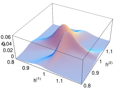
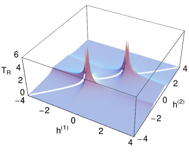
This is simply a quadratic approximation, that does not rely on the CLT. Its validity requires t2σ21much-less-thansuperscript𝑡2superscript𝜎21t^{2}\sigma^{2}\ll 1 that in turn implies t1/H2much-less-than𝑡1delimited-⟨⟩subscript𝐻2t\ll 1/\sqrt{\left\langle H_{2}\right\rangle} (as will be explained later this means roughly tLd/2much-less-than𝑡superscript𝐿𝑑2t\ll L^{-d/2} where d𝑑d is the space dimension). From figure 1 we see that typically (t)𝑡\mathcal{L}\left(t\right) decays from 1 and after an initial transient, starts oscillating around an average value ¯¯\overline{\mathcal{L}} which will be computed below. Now, when the CLT applies, equation (7) can help us to define this transient or relaxation time TRsubscript𝑇𝑅T_{R} given by eTR2σ2=¯superscript𝑒superscriptsubscript𝑇𝑅2superscript𝜎2¯e^{-T_{R}^{2}\sigma^{2}}=\overline{\mathcal{L}}. Roughly after this time one starts seeing oscillations in (t)𝑡\mathcal{L}\left(t\right). Since in general (see below) one has ¯efLdsimilar-to-or-equals¯superscript𝑒𝑓superscript𝐿𝑑\overline{\mathcal{L}}\simeq e^{-fL^{d}}, and when the CLT applies σ2superscript𝜎2\sigma^{2} scales like the system volume, the relaxation time scales as TR=ln¯/σ2=O(L0)subscript𝑇𝑅¯superscript𝜎2𝑂superscript𝐿0T_{R}=\sqrt{-\ln\overline{\mathcal{L}}/\sigma^{2}}=O\left(L^{0}\right). The situation is different when one considers small variations of the parameters δh𝛿\delta h. In this limit the average LE is related to the well studied ground state fidelity F=|ψ(1)|ψ(2)|𝐹inner-productsuperscript𝜓1superscript𝜓2F=\left|\langle\psi^{\left(1\right)}|\psi^{\left(2\right)}\rangle\right|. More precisely one has ¯F4similar-to-or-equals¯superscript𝐹4\overline{\mathcal{L}}\simeq F^{4} Rossini et al. (2007b). Close to critical points the behavior of the fidelity is dictated by the scaling dimension ΔΔ\Delta of the most relevant operator in H𝐻H with respect to the critical state |ψket𝜓|\psi\rangle Campos Venuti and Zanardi (2007). The precise scaling is the following: F1const.×δh2L2(d+ζΔ)F\sim 1-\mathrm{const.}\times\delta h^{2}L^{2\left(d+\zeta-\Delta\right)}, where ζ𝜁\zeta is the dynamical critical exponent. Similarly one can show (see below) that σ2L2(dΔ)similar-tosuperscript𝜎2superscript𝐿2𝑑Δ\sigma^{2}\sim L^{2\left(d-\Delta\right)}. All in all this amounts to saying that the relaxation time for small variation δh𝛿\delta h around a critical point (roughly δhL(d+ζΔ)much-less-than𝛿superscript𝐿𝑑𝜁Δ\delta h\ll L^{-\left(d+\zeta-\Delta\right)}) increases from O(1)𝑂1O\left(1\right) to TRLζsimilar-tosubscript𝑇𝑅superscript𝐿𝜁T_{R}\sim L^{\zeta}. In the thermodynamic limit instead, i.e. taking first the limit L𝐿L\to\infty, using standard scaling arguments, one can show that for δh𝛿\delta h small and hh close to the critical point hcsubscript𝑐h_{c}, the relaxation times diverges as TR|hhc|ζνsimilar-tosubscript𝑇𝑅superscriptsubscript𝑐𝜁𝜈T_{R}\sim\left|h-h_{c}\right|^{-\zeta\nu}, ν𝜈\nu being the correlation length exponent. In figure 2 we plot the relaxation time for a concrete example that will be studied thoroughly in section III, the Ising model in transverse field. There one has Δ=ζ=ν=1Δ𝜁𝜈1\Delta=\zeta=\nu=1, and so the singularities observed in figure 2 are of simple algebraic type: TR|hhc|1similar-tosubscript𝑇𝑅superscriptsubscript𝑐1T_{R}\sim\left|h-h_{c}\right|^{-1} around the critical points hc=±1subscript𝑐plus-or-minus1h_{c}=\pm 1.

Let us now turn to discuss when we expect the CLT to work. Consider first the case when |ψket𝜓|\psi\rangle is the ground state of a gapped Hamiltonian and the connected energy correlators go to zero exponentially fast: H(x)H(y)|xy|H(x)H(y)superscript𝑥𝑦delimited-⟨⟩𝐻𝑥𝐻𝑦delimited-⟨⟩𝐻𝑥delimited-⟨⟩𝐻𝑦\langle H\left(x\right)H\left(y\right)\rangle\stackrel{{\scriptstyle\left|x-y\right|\to\infty}}{{\longrightarrow}}\langle H\left(x\right)\rangle\langle H\left(y\right)\rangle (exponential clustering). In this case the connected averages of H𝐻H scale as the volume: HncLdsimilar-tosubscriptdelimited-⟨⟩superscript𝐻𝑛𝑐superscript𝐿𝑑\left\langle H^{n}\right\rangle_{c}\sim L^{d}. As a consequence the cumulants of the rescaled variable satisfy YncL(nd2d)/2similar-tosubscriptdelimited-⟨⟩superscript𝑌𝑛𝑐superscript𝐿𝑛𝑑2𝑑2\left\langle Y^{n}\right\rangle_{c}\sim L^{-\left(nd-2d\right)/2} for n2𝑛2n\geq 2, which immediately implies the CLT in the sense given above.

Therefore we can have violation of the CLT only in the gapless case when the state |ψket𝜓|\psi\rangle is critical or when clustering fails. Let us then consider a critical state |ψket𝜓|\psi\rangle. Connected averages have a regular extensive part and a singular part which scales according to the most relevant component of H𝐻H with scaling dimension ΔΔ\Delta. When |ψket𝜓|\psi\rangle is the ground state of H𝐻H at a different coupling, ΔΔ\Delta is the scaling dimension of the perturbation δH𝛿𝐻\delta H to the critical Hamiltonian. At leading order, we can write HncAnLd+BnLn(dΔ)similar-tosubscriptdelimited-⟨⟩superscript𝐻𝑛𝑐subscript𝐴𝑛superscript𝐿𝑑subscript𝐵𝑛superscript𝐿𝑛𝑑Δ\left\langle H^{n}\right\rangle_{c}\sim A_{n}L^{d}+B_{n}L^{n\left(d-\Delta\right)}, and so the rescaled variable satisfies

YncAnLd+BnLn(dΔ)(A2Ld+B2L2(dΔ))n/2.similar-tosubscriptdelimited-⟨⟩superscript𝑌𝑛𝑐subscript𝐴𝑛superscript𝐿𝑑subscript𝐵𝑛superscript𝐿𝑛𝑑Δsuperscriptsubscript𝐴2superscript𝐿𝑑subscript𝐵2superscript𝐿2𝑑Δ𝑛2\left\langle Y^{n}\right\rangle_{c}\sim\frac{A_{n}L^{d}+B_{n}L^{n\left(d-\Delta\right)}}{\left(A_{2}L^{d}+B_{2}L^{2\left(d-\Delta\right)}\right)^{n/2}}.

If Δ<d/2Δ𝑑2\Delta<d/2 the cumulants of the rescaled variable Y𝑌Y don’t go to zero but to universal constants Privman et al. ; Aji and Goldenfeld (2001) given by

YncBnB2n/2.subscriptdelimited-⟨⟩superscript𝑌𝑛𝑐subscript𝐵𝑛superscriptsubscript𝐵2𝑛2\left\langle Y^{n}\right\rangle_{c}\to\frac{B_{n}}{B_{2}^{n/2}}.

In this case the probability distribution of the energy is a, non-Gaussian, universal distribution. This kind of universal behavior has been observed for instance in Lamacraft and Fendley (2008) on an example where the scaling dimension is Δ=1/8Δ18\Delta=1/8. In the opposite situation where Δ>d/2Δ𝑑2\Delta>d/2, all the cumulants of Y𝑌Y go to zero except for the first two, and the distribution function approaches a Gaussian in the large size limit. In the intermediate case Δ=d/2Δ𝑑2\Delta=d/2 the cumulants of Y𝑌Y do not go zero but to a constant which is however not universal due to extensive contributions coming from the denominator. We recall that in d𝑑d dimensional, zero temperature quantum mechanics, operators are classified into relevant, irrelevant, and marginal if their scaling dimension is respectively smaller, larger, or equal to d+ζ𝑑𝜁d+\zeta where ζ𝜁\zeta is the dynamical exponent. Hence we see that, even in the critical case, we observe deviation from the Gaussian behavior only if the perturbation δH𝛿𝐻\delta H is sufficiently relevant, specifically Δ<d/2Δ𝑑2\Delta<d/2.

To finish let us remind the reader that the CLT also breaks down when clustering fails.

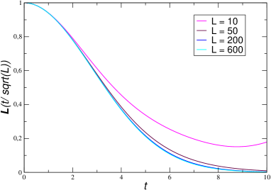
To summarize, when the CLT applies, the LE tends to a Gaussian and plotting the function L(t/H22)subscript𝐿𝑡subscriptdelimited-⟨⟩superscript𝐻22\mathcal{L}_{L}\left(t/\sqrt{\left\langle H^{2}\right\rangle_{2}}\right) for different sizes L𝐿L one should observe data collapse (see figure 3).
Refer to caption
Figure 2: (Color online) Relaxation time for the Loschmidt echo in the Ising model in transverse field. The critical points are at hc=±1.subscript𝑐plus-or-minus1h_{c}=\pm 1.Clearly we observe divergences at critical points when δh𝛿\delta h is small. On the line h(1)=h(2)superscript1superscript2h^{\left(1\right)}=h^{\left(2\right)} (t)=1𝑡1\mathcal{L}\left(t\right)=1 and so there is no relaxation or even dynamics.
Refer to caption
Figure 3: (Color online) Rescaled Loschmidt echo L(t/L)subscript𝐿𝑡𝐿\mathcal{L}_{L}\left(t/\sqrt{L}\right) for the Ising model in transverse field. System sizes are, from top to bottom, L=10,50,200,600𝐿1050200600L=10,50,200,600. The state which defines the average is critical: h(1)=1superscript11h^{\left(1\right)}=1 while H𝐻H is at h(2)=2.5superscript22.5h^{\left(2\right)}=2.5. The same data collapse feature is observed when choosing different h(i)superscript𝑖h^{\left(i\right)}s, although the variance of this Gaussian is sensitive to that.

II.3 Equilibration and long time behavior

After having discussed the short time behavior of the LE related to the initial transient, let us now turn to its long time behavior.

We first re-write Eq. (3) in the eigenbasis of H=nEn|nn|𝐻subscript𝑛subscript𝐸𝑛ket𝑛bra𝑛H=\sum_{n}E_{n}|n\rangle\langle n|

(t)=n,mpnpmeit(EnEm),𝑡subscript𝑛𝑚subscript𝑝𝑛subscript𝑝𝑚superscript𝑒𝑖𝑡subscript𝐸𝑛subscript𝐸𝑚\mathcal{L}\left(t\right)=\sum_{n,m}p_{n}p_{m}e^{-it\left(E_{n}-E_{m}\right)}, (8)

where pn=|ψ|n|2subscript𝑝𝑛superscriptinner-product𝜓𝑛2p_{n}=\left|\langle\psi|n\rangle\right|^{2}.

If the spectrum of H𝐻H is non degenerate the superoperator 𝒫(1)superscript𝒫1{\cal P}^{(1)} acts as a dephasing in the Hamiltonian eigenbasis i.e, 𝒫(1)(X)=nn|X|n|nn|.superscript𝒫1𝑋subscript𝑛quantum-operator-product𝑛𝑋𝑛ket𝑛bra𝑛{\cal P}^{(1)}(X)=\sum_{n}\langle n|X|n\rangle|n\rangle\langle n|. In other words the time average of the exponentials in Eq. (8) gives simply δn,msubscript𝛿𝑛𝑚\delta_{n,m} and equation (4) reduces to ¯=npn2¯subscript𝑛superscriptsubscript𝑝𝑛2\overline{\mathcal{L}}=\sum_{n}p_{n}^{2}. As is well known this quantity is the purity of an equilibrium, dephased, state: ρeq=npn|nn|subscript𝜌eqsubscript𝑛subscript𝑝𝑛ket𝑛bra𝑛\rho_{\mathrm{eq}}=\sum_{n}p_{n}|n\rangle\langle n|.

Time scales

In the preceding section we already defined a relevant time scale, the relaxation time TRsubscript𝑇𝑅T_{R} which is O(1)𝑂1O\left(1\right) off-criticality while TR=O(Lζ)subscript𝑇𝑅𝑂superscript𝐿𝜁T_{R}=O\left(L^{\zeta}\right) in the critical case and for sufficiently small variations δhL(d+ζΔ)much-less-than𝛿superscript𝐿𝑑𝜁Δ\delta h\ll L^{-\left(d+\zeta-\Delta\right)}.

In some situations it is useful to consider a finite observation time T𝑇T. We will write ¯¯\overline{\mathcal{L}} to indicate the corresponding average. It is natural to ask about the interplay between the observation time T𝑇T and the linear size of the system L𝐿L. In other words in general limLlimTL¯limTlimLL¯subscript𝐿subscript𝑇¯subscript𝐿subscript𝑇subscript𝐿¯subscript𝐿\lim_{L\to\infty}\lim_{T\to\infty}\overline{\mathcal{L}_{L}}\neq\lim_{T\to\infty}\lim_{L\to\infty}\overline{\mathcal{L}_{L}}. Since taking larger system sizes has the effect of sending the revival times to infinity and the LE attunes its maximum value 111 at t=0𝑡0t=0, typically the function limLL(t)subscript𝐿subscript𝐿𝑡\lim_{L\to\infty}\mathcal{L}_{L}\left(t\right) has only one large peak at t=0𝑡0t=0 whereas L(t)subscript𝐿𝑡\mathcal{L}_{L}\left(t\right) has peaks at all the revival times. Correspondingly we expect limLlimTL¯>limTlimLL¯subscript𝐿subscript𝑇¯subscript𝐿subscript𝑇subscript𝐿¯subscript𝐿\lim_{L\to\infty}\lim_{T\to\infty}\overline{\mathcal{L}_{L}}>\lim_{T\to\infty}\lim_{L\to\infty}\overline{\mathcal{L}_{L}}. This expectation has been confirmed for the case of the one dimensional quantum Ising model, see section III.

Another question which is relevant in the measurement process is how large must the observation time be to effectively measure ¯¯\overline{\mathcal{L}}? That is, what is the condition to have T1¯=¯¯superscriptsubscript𝑇1¯\overline{\mathcal{L}^{T_{1}}}=\overline{\mathcal{L}} or more in general what is the smallest time Tnsubscript𝑇𝑛T_{n} such that one observes [()n]Tn¯=()n¯¯superscriptdelimited-[]superscript𝑛subscript𝑇𝑛¯superscript𝑛\overline{\left[\left(\mathcal{L}\right)^{n}\right]^{T_{n}}}=\overline{\left(\mathcal{L}\right)^{n}}? Let us focus on T1subscript𝑇1T_{1}. Looking at equation (8) one realizes that it suffices to have TΔmin1much-greater-than𝑇superscriptsubscriptΔmin1T\gg\Delta_{\mathrm{min}}^{-1}, where ΔminsubscriptΔmin\Delta_{\mathrm{min}} is the smallest gap in the whole spectrum i.e. Δmin=minn,m(EnEm)subscriptΔminsubscript𝑛𝑚subscript𝐸𝑛subscript𝐸𝑚\Delta_{\mathrm{min}}=\min_{n,m}\left(E_{n}-E_{m}\right). We can address this question for the class of quasi-free Fermi systems in d𝑑d spatial dimensions. In this case the energy has the form En=𝒌n𝒌Λ𝒌subscript𝐸𝑛subscript𝒌subscript𝑛𝒌subscriptΛ𝒌E_{n}=\sum_{\boldsymbol{k}}n_{\boldsymbol{k}}\Lambda_{\boldsymbol{k}} where 𝒌𝒌\boldsymbol{k} is a d𝑑d-dimensional quasi-momentum-like label and we can assume the one particle energy Λ𝒌subscriptΛ𝒌\Lambda_{\boldsymbol{k}} to be positive. Then the gap is given by Δmin=minβ𝒌|𝒌β𝒌Λ𝒌|subscriptΔminsubscriptsubscript𝛽𝒌subscript𝒌subscript𝛽𝒌subscriptΛ𝒌\Delta_{\mathrm{min}}=\min_{\beta_{\boldsymbol{k}}}\left|\sum_{\boldsymbol{k}}\beta_{\boldsymbol{k}}\Lambda_{\boldsymbol{k}}\right| with β𝒌=0,±1subscript𝛽𝒌0plus-or-minus1\beta_{\boldsymbol{k}}=0,\pm 1. By choosing β𝒌=(1)𝒌subscript𝛽𝒌superscript1𝒌\beta_{\boldsymbol{k}}=\left(-1\right)^{\boldsymbol{k}} , one obtains a ΔminsubscriptΔmin\Delta_{\mathrm{min}} which is exponentially small in L𝐿L in those (frequent) cases where Λ𝒌subscriptΛ𝒌\Lambda_{\boldsymbol{k}} is an analytic function of 𝒌𝒌\boldsymbol{k} not (c). However in quasi free systems the weights pnsubscript𝑝𝑛p_{n} decrease exponentially with the number of excitations in n𝑛n. In practice the highest weight is given for energy differences between the one and zero particle spectra: Δ(1,0)=min𝒌Λ𝒌superscriptΔ10subscript𝒌subscriptΛ𝒌\Delta^{\left(1,0\right)}=\min_{\boldsymbol{k}}\Lambda_{\boldsymbol{k}} which is a constant of order 1 in the gapful case, while typically scales as L1superscript𝐿1L^{-1} for the critical case. The next largest amount of spectral weight is attained at a gap which is a difference between one particle energies Δ(1,1)=min𝒌,𝒒|Λ𝒌Λ𝒒|superscriptΔ11subscript𝒌𝒒subscriptΛ𝒌subscriptΛ𝒒\Delta^{\left(1,1\right)}=\min_{\boldsymbol{k},\boldsymbol{q}}\left|\Lambda_{\boldsymbol{k}}-\Lambda_{\boldsymbol{q}}\right|. It will be favorable to have 𝒌𝒌\boldsymbol{k} and 𝒒𝒒\boldsymbol{q} nearby in the region where Λ𝒌subscriptΛ𝒌\Lambda_{\boldsymbol{k}} is flat or almost flat. So we get Δ(1,1)=min𝒌|Λ𝒌Λ𝒌+δ𝒌|min𝒌|𝒌Λ𝒌δ𝒌|superscriptΔ11subscript𝒌subscriptΛ𝒌subscriptΛ𝒌𝛿𝒌similar-to-or-equalssubscript𝒌subscript𝒌subscriptΛ𝒌𝛿𝒌\Delta^{\left(1,1\right)}=\min_{\boldsymbol{k}}\left|\Lambda_{\boldsymbol{k}}-\Lambda_{\boldsymbol{k}+\delta\boldsymbol{k}}\right|\simeq\min_{\boldsymbol{k}}\left|\nabla_{\boldsymbol{k}}\Lambda_{\boldsymbol{k}}\cdot\delta\boldsymbol{k}\right|. This gap is at least of order of L2superscript𝐿2L^{-2} (or at least O(L3)𝑂superscript𝐿3O\left(L^{-3}\right) if there exists a 𝒌𝒌\boldsymbol{k}-vector such that 𝒌Λ𝒌=0subscript𝒌subscriptΛ𝒌0\nabla_{\boldsymbol{k}}\Lambda_{\boldsymbol{k}}=0). From this discussion we estimate that, at least in quasi-free systems, to have T1¯¯similar-to-or-equals¯superscriptsubscript𝑇1¯\overline{\mathcal{L}^{T_{1}}}\simeq\overline{\mathcal{L}} one must take T1=O(1)subscript𝑇1𝑂1T_{1}=O\left(1\right) in the gapful case, while one has T1=O(L)subscript𝑇1𝑂𝐿T_{1}=O\left(L\right) at criticality. If one needs T1¯¯similar-to-or-equals¯superscriptsubscript𝑇1¯\overline{\mathcal{L}^{T_{1}}}\simeq\overline{\mathcal{L}} with a larger degree of precision than one must choose considerably larger time: T1=O(L2)subscript𝑇1𝑂superscript𝐿2T_{1}=O\left(L^{2}\right) (or T1=O(L3)subscript𝑇1𝑂superscript𝐿3T_{1}=O\left(L^{3}\right) if 𝒌Λ𝒌=0subscript𝒌subscriptΛ𝒌0\nabla_{\boldsymbol{k}}\Lambda_{\boldsymbol{k}}=0 has a solution within the allowed set of 𝒌𝒌\boldsymbol{k}-vectors). Related time scales are revival times. We define a revival time to be that particular time for which a large portion of spectral weight pnpmsubscript𝑝𝑛subscript𝑝𝑚p_{n}p_{m} has revived. More precisely Trevωpeak=2πsubscript𝑇revsubscript𝜔peak2𝜋T_{\mathrm{rev}}\omega_{\mathrm{peak}}=2\pi, where ωpeaksubscript𝜔peak\omega_{\mathrm{peak}} is a particular frequency EnEmsubscript𝐸𝑛subscript𝐸𝑚E_{n}-E_{m} such that the weight pnpmsubscript𝑝𝑛subscript𝑝𝑚p_{n}p_{m} is large. From the discussion above we expect Trev=O(1)subscript𝑇rev𝑂1T_{\mathrm{rev}}=O\left(1\right) when H𝐻H has a gap above the ground state, while Trev=O(L)subscript𝑇rev𝑂𝐿T_{\mathrm{rev}}=O\left(L\right) when H𝐻H is critical. These expectations have been confirmed (see figure 1) on the hand of a solvable model that will be discussed in the next sections.

II.4 Moments of the Loschmidt echo

Having computed the time averaged LE we can now turn to higher moments. In doing this one has to distinguish cases where n=m𝑛𝑚n=m from those where En=Emsubscript𝐸𝑛subscript𝐸𝑚E_{n}=E_{m} in Eq. (8). So we write

(t)𝑡\displaystyle\mathcal{L}\left(t\right) =\displaystyle= ¯+X(t),¯𝑋𝑡\displaystyle\overline{\mathcal{L}}+X\left(t\right),
X(t)𝑋𝑡\displaystyle X\left(t\right) =\displaystyle= nmpnpmeit(EnEm),subscript𝑛𝑚subscript𝑝𝑛subscript𝑝𝑚superscript𝑒𝑖𝑡subscript𝐸𝑛subscript𝐸𝑚\displaystyle\sum_{n\neq m}p_{n}p_{m}e^{-it\left(E_{n}-E_{m}\right)},

and the n𝑛n-th moment is given by

[(t)]n¯=k=0n(nk)¯nk[X(t)]k¯.¯superscriptdelimited-[]𝑡𝑛superscriptsubscript𝑘0𝑛𝑛𝑘superscript¯𝑛𝑘¯superscriptdelimited-[]𝑋𝑡𝑘\overline{\left[\mathcal{L}\left(t\right)\right]^{n}}=\sum_{k=0}^{n}\left(\begin{array}[]{c}n\\ k\end{array}\right)\overline{\mathcal{L}}^{n-k}\overline{\left[X\left(t\right)\right]^{k}}.

The computation of the average [X(t)]k¯¯superscriptdelimited-[]𝑋𝑡𝑘\overline{\left[X\left(t\right)\right]^{k}} can be done assuming a strong non-resonance condition. With this we mean the following. We say H𝐻H satisfies a k𝑘k-non-resonance condition if the only way to fulfill l=1kEilEjl=0superscriptsubscript𝑙1𝑘subscript𝐸subscript𝑖𝑙subscript𝐸subscript𝑗𝑙0\sum_{l=1}^{k}E_{i_{l}}-E_{j_{l}}=0 is to match the Eisubscript𝐸𝑖E_{i}’s to the Ejsubscript𝐸𝑗E_{j}’s. Strong non resonance is k𝑘k-non-resonance for any k𝑘k. Note that this condition cannot be fulfilled when k𝑘k becomes of the order of the Hilbert’s space dimension. Now to compute [X(t)]k¯¯superscriptdelimited-[]𝑋𝑡𝑘\overline{\left[X\left(t\right)\right]^{k}} draw 2k2𝑘2k points in two rows of length k𝑘k. Imagine Eisubscript𝐸𝑖E_{i} (Ejsubscript𝐸𝑗E_{j}) are the points at the left (right). Now draw all possible contraction between i𝑖i’s and j𝑗j’s (no contraction among i𝑖i’s or j𝑗j’s since they have the same sing), which are k!𝑘k!, but keep only those sets of contractions where there is no horizontal line. This requirement corresponds to the constraint iljl,l=1,,kformulae-sequencesubscript𝑖𝑙subscript𝑗𝑙𝑙1𝑘i_{l}\neq j_{l},\,\,l=1,\ldots,k. For example for [X(t)]2superscriptdelimited-[]𝑋𝑡2\left[X\left(t\right)\right]^{2} we have only one contribution

[Uncaptioned image]

so

[X(t)]2¯=i1i2pi12pi22¯superscriptdelimited-[]𝑋𝑡2subscriptsubscript𝑖1subscript𝑖2superscriptsubscript𝑝subscript𝑖12superscriptsubscript𝑝subscript𝑖22\overline{\left[X\left(t\right)\right]^{2}}=\sum_{i_{1}\neq i_{2}}p_{i_{1}}^{2}p_{i_{2}}^{2}

For [X(t)]3¯¯superscriptdelimited-[]𝑋𝑡3\overline{\left[X\left(t\right)\right]^{3}} we have two diagrams:

[Uncaptioned image]

Both these diagrams give the same contribution (simply swap i𝑖i’s with j𝑗j’s) and the result is

[X(t)]3¯=2i1i2i2i3,i3i1pi12pi22pi32.¯superscriptdelimited-[]𝑋𝑡32subscriptsubscript𝑖1subscript𝑖2formulae-sequencesubscript𝑖2subscript𝑖3subscript𝑖3subscript𝑖1superscriptsubscript𝑝subscript𝑖12superscriptsubscript𝑝subscript𝑖22superscriptsubscript𝑝subscript𝑖32\overline{\left[X\left(t\right)\right]^{3}}=2\sum_{\begin{subarray}{c}i_{1}\neq i_{2}\\ i_{2}\neq i_{3},i_{3}\neq i_{1}\end{subarray}}p_{i_{1}}^{2}p_{i_{2}}^{2}p_{i_{3}}^{2}.

The number of terms in [X(t)]k¯¯superscriptdelimited-[]𝑋𝑡𝑘\overline{\left[X\left(t\right)\right]^{k}}, N(k)𝑁𝑘N\left(k\right) is the number of all permutations without fixed points and is given by

N(k)=j=2k(1)kj(kj)(j!1).𝑁𝑘superscriptsubscript𝑗2𝑘superscript1𝑘𝑗𝑘𝑗𝑗1N\left(k\right)=\sum_{j=2}^{k}\left(-1\right)^{k-j}\left(\begin{array}[]{c}k\\ j\end{array}\right)\left(j!-1\right).

However, among these N(k)𝑁𝑘N\left(k\right) terms, many of them give different contributions. Look for instance at [X(t)]4¯¯superscriptdelimited-[]𝑋𝑡4\overline{\left[X\left(t\right)\right]^{4}}:

[X(t)]4¯=3(i1i2pi12pi22)2+6i1i2,i2i3i3i4,i4i1pi12pi22pi32pi42¯superscriptdelimited-[]𝑋𝑡43superscriptsubscriptsubscript𝑖1subscript𝑖2superscriptsubscript𝑝subscript𝑖12superscriptsubscript𝑝subscript𝑖2226subscriptformulae-sequencesubscript𝑖1subscript𝑖2subscript𝑖2subscript𝑖3formulae-sequencesubscript𝑖3subscript𝑖4subscript𝑖4subscript𝑖1superscriptsubscript𝑝subscript𝑖12superscriptsubscript𝑝subscript𝑖22superscriptsubscript𝑝subscript𝑖32superscriptsubscript𝑝subscript𝑖42\overline{\left[X\left(t\right)\right]^{4}}=3\left(\sum_{i_{1}\neq i_{2}}p_{i_{1}}^{2}p_{i_{2}}^{2}\right)^{2}+6\sum_{\begin{subarray}{c}i_{1}\neq i_{2},i_{2}\neq i_{3}\\ i_{3}\neq i_{4},i_{4}\neq i_{1}\end{subarray}}p_{i_{1}}^{2}p_{i_{2}}^{2}p_{i_{3}}^{2}p_{i_{4}}^{2}

Correctly one has 3+6=N(4)=936𝑁493+6=N\left(4\right)=9.

We collect here the first three moments

μ1subscript𝜇1\displaystyle\mu_{1} =\displaystyle= ¯¯\displaystyle\overline{\mathcal{L}}
μ2subscript𝜇2\displaystyle\mu_{2} =\displaystyle= ¯2+i1i2pi12pi22superscript¯2subscriptsubscript𝑖1subscript𝑖2superscriptsubscript𝑝subscript𝑖12superscriptsubscript𝑝subscript𝑖22\displaystyle\overline{\mathcal{L}}^{2}+\sum_{i_{1}\neq i_{2}}p_{i_{1}}^{2}p_{i_{2}}^{2}
μ3subscript𝜇3\displaystyle\mu_{3} =\displaystyle= ¯3+3¯i1i2pi12pi22+2i1i2i2i3,i3i1pi12pi22pi32superscript¯33¯subscriptsubscript𝑖1subscript𝑖2superscriptsubscript𝑝subscript𝑖12superscriptsubscript𝑝subscript𝑖222subscriptsubscript𝑖1subscript𝑖2formulae-sequencesubscript𝑖2subscript𝑖3subscript𝑖3subscript𝑖1superscriptsubscript𝑝subscript𝑖12superscriptsubscript𝑝subscript𝑖22superscriptsubscript𝑝subscript𝑖32\displaystyle\overline{\mathcal{L}}^{3}+3\overline{\mathcal{L}}\sum_{i_{1}\neq i_{2}}p_{i_{1}}^{2}p_{i_{2}}^{2}+2\sum_{\begin{subarray}{c}i_{1}\neq i_{2}\\ i_{2}\neq i_{3},i_{3}\neq i_{1}\end{subarray}}p_{i_{1}}^{2}p_{i_{2}}^{2}p_{i_{3}}^{2}

while the cumulants are

κ1subscript𝜅1\displaystyle\kappa_{1} =\displaystyle= ¯¯\displaystyle\overline{\mathcal{L}}
κ2subscript𝜅2\displaystyle\kappa_{2} =\displaystyle= i1i2pi12pi22subscriptsubscript𝑖1subscript𝑖2superscriptsubscript𝑝subscript𝑖12superscriptsubscript𝑝subscript𝑖22\displaystyle\sum_{i_{1}\neq i_{2}}p_{i_{1}}^{2}p_{i_{2}}^{2}
κ3subscript𝜅3\displaystyle\kappa_{3} =\displaystyle= 2i1i2i2i3,i3i1pi12pi22pi32.2subscriptsubscript𝑖1subscript𝑖2formulae-sequencesubscript𝑖2subscript𝑖3subscript𝑖3subscript𝑖1superscriptsubscript𝑝subscript𝑖12superscriptsubscript𝑝subscript𝑖22superscriptsubscript𝑝subscript𝑖32\displaystyle 2\sum_{\begin{subarray}{c}i_{1}\neq i_{2}\\ i_{2}\neq i_{3},i_{3}\neq i_{1}\end{subarray}}p_{i_{1}}^{2}p_{i_{2}}^{2}p_{i_{3}}^{2}.

We can notice that each term in [X(t)]k¯¯superscriptdelimited-[]𝑋𝑡𝑘\overline{\left[X\left(t\right)\right]^{k}} has the same form of ¯ksuperscript¯𝑘\overline{\mathcal{L}}^{k} except for a number of non-resonance constraints of the form ilimsubscript𝑖𝑙subscript𝑖𝑚i_{l}\neq i_{m}. Correspondingly [X(t)]k¯<N(k)¯k¯superscriptdelimited-[]𝑋𝑡𝑘𝑁𝑘superscript¯𝑘\overline{\left[X\left(t\right)\right]^{k}}<N\left(k\right)\overline{\mathcal{L}}^{k} . Using now k=0n(nk)N(k)=n!superscriptsubscript𝑘0𝑛𝑛𝑘𝑁𝑘𝑛\sum_{k=0}^{n}\left(\begin{array}[]{c}n\\ k\end{array}\right)N\left(k\right)=n! we obtain the simple bound n¯<n!¯n¯superscript𝑛𝑛superscript¯𝑛\overline{\mathcal{L}^{n}}<n!\overline{\mathcal{L}}^{n} for n2𝑛2n\geq 2. This means that

eλ¯χ~(λ)=eλ¯<11¯λ,superscript𝑒𝜆¯~𝜒𝜆¯superscript𝑒𝜆11¯𝜆e^{\lambda\overline{\mathcal{L}}}\leq\tilde{\chi}\left(\lambda\right)=\overline{e^{\lambda\mathcal{L}}}<\frac{1}{1-\overline{\mathcal{L}}\lambda},

and so we obtained a bound on the characteristic function χ~~𝜒\tilde{\chi}. We see that, when ¯0¯0\overline{\mathcal{L}}\to 0 the probability distribution of \mathcal{L} becomes a delta function at zero (the characteristic function becomes identically one). The distribution function of the upper bound is

ϑ(x)ex/¯¯.italic-ϑ𝑥superscript𝑒𝑥¯¯\vartheta\left(x\right)\frac{e^{-x/\overline{\mathcal{L}}}}{\overline{\mathcal{L}}}.

Later we will encounter situations where this function gives a good approximation to the Loschmidt echo probability distribution.

III Ising Model in Transverse Field

From now on we will give a detailed description of the Loschmidt echo for the case of an exactly solvable model. The model we consider is the Ising model in transverse field with Hamiltonian

H=i(σixσi+1x+hσiz).𝐻subscript𝑖superscriptsubscript𝜎𝑖𝑥superscriptsubscript𝜎𝑖1𝑥superscriptsubscript𝜎𝑖𝑧H=-\sum_{i}\left(\sigma_{i}^{x}\sigma_{i+1}^{x}+h\sigma_{i}^{z}\right).

This model can be mapped to quasi-free fermions and so diagonalized exactly. At zero temperature we distinguish two phases: i) An ordered one in the longitudinal direction in which σixσjx|ij|m2superscript𝑖𝑗delimited-⟨⟩superscriptsubscript𝜎𝑖𝑥superscriptsubscript𝜎𝑗𝑥superscript𝑚2\langle\sigma_{i}^{x}\sigma_{j}^{x}\rangle\stackrel{{\scriptstyle\left|i-j\right|\to\infty}}{{\longrightarrow}}m^{2}, for |h|<11\left|h\right|<1, and ii) A paramagnetic phase for |h|>11\left|h\right|>1. The points |h|=11\left|h\right|=1 are critical points where the system is described by a conformal invariant field theory with central charge c=1/2𝑐12c=1/2.

The LE is given in this case by Quan et al. (2006b) (superscript, inserted here for clarity, refer to different values of the coupling constant hh)

(t)𝑡\displaystyle\mathcal{L}\left(t\right) =\displaystyle= |ψ(1)|eitH(2)|ψ(1)|2superscriptquantum-operator-productsuperscript𝜓1superscript𝑒𝑖𝑡superscript𝐻2superscript𝜓12\displaystyle\left|\langle\psi^{\left(1\right)}|e^{-itH^{\left(2\right)}}|\psi^{\left(1\right)}\rangle\right|^{2} (9)
=\displaystyle= k>0(1sin2(ϑk(1)ϑk(2))sin2(Λk(2)t/2))subscriptproduct𝑘01superscript2superscriptsubscriptitalic-ϑ𝑘1superscriptsubscriptitalic-ϑ𝑘2superscript2superscriptsubscriptΛ𝑘2𝑡2\displaystyle\prod_{k>0}\left(1-\sin^{2}\left(\vartheta_{k}^{(1)}-\vartheta_{k}^{\left(2\right)}\right)\sin^{2}\left(\Lambda_{k}^{\left(2\right)}t/2\right)\right)

where tan(ϑk(i))=sin(k)/(h(i)+cos(k))superscriptsubscriptitalic-ϑ𝑘𝑖𝑘superscript𝑖𝑘\tan\left(\vartheta_{k}^{\left(i\right)}\right)=-\sin\left(k\right)/\left(h^{\left(i\right)}+\cos\left(k\right)\right) and the single particle fermionic dispersion is Λk(i)=2(h(i)+cos(k))2+sin(k)2\Lambda_{k}^{\left(i\right)}=2\sqrt{\left(h^{\left(i\right)}+\cos\left(k\right)\right)^{2}+\sin\left(k\right)^{2}}. The band minimum (maximum) is at Em=2min{|1h(2)|,|1+h(2)|}subscript𝐸𝑚21superscript21superscript2E_{m}=2\min\left\{\left|1-h^{\left(2\right)}\right|,\left|1+h^{\left(2\right)}\right|\right\} (EM=2max{|1h(2)|,|1+h(2)|}subscript𝐸𝑀21superscript21superscript2E_{M}=2\max\left\{\left|1-h^{\left(2\right)}\right|,\left|1+h^{\left(2\right)}\right|\right\}). Finally, for periodic boundary conditions that will be used throughout, the quasi-momenta satisfy kn=π(2n+1)/Lsubscript𝑘𝑛𝜋2𝑛1𝐿k_{n}=\pi\left(2n+1\right)/L, n=0,1,,L/21𝑛01𝐿21n=0,1,\ldots,L/2-1. Exploiting the fact that H𝐻H decomposes into a direct sum of L/2𝐿2L/2 blocks 4×4444\times 4, we are able to compute the complete dephased equilibrium state ρeq=npn|nn|subscript𝜌eqsubscript𝑛subscript𝑝𝑛ket𝑛bra𝑛\rho_{\mathrm{eq}}=\sum_{n}p_{n}|n\rangle\langle n|. The result is

ρeq=α2Lp(α)|αα|,subscript𝜌eqsubscript𝛼superscriptsubscript2𝐿𝑝𝛼ket𝛼bra𝛼\rho_{\mathrm{eq}}=\sum_{\alpha\in\mathbb{Z}_{2}^{L}}p\left(\alpha\right)|\alpha\rangle\langle\alpha|, (10)

where the multi-index α𝛼\alpha is α=(α1,,αL)𝛼subscript𝛼1subscript𝛼𝐿\alpha=\left(\alpha_{1},\ldots,\alpha_{L}\right), αi=0,1subscript𝛼𝑖01\alpha_{i}=0,1, the state is |α=k>0|αk|\alpha\rangle=\otimes_{k>0}|\alpha_{k}\rangle with |0k=cos(ϑ(2)/2)|0,0k,kisin(ϑ(2)/2)|1,1k,kketsubscript0𝑘superscriptitalic-ϑ22subscriptket00𝑘𝑘𝑖superscriptitalic-ϑ22subscriptket11𝑘𝑘|0_{k}\rangle=\cos\left(\vartheta^{\left(2\right)}/2\right)|0,0\rangle_{k,-k}-i\sin\left(\vartheta^{\left(2\right)}/2\right)|1,1\rangle_{k,-k} and |0k=isin(ϑ(2)/2)|0,0k,kcos(ϑ(2)/2)|1,1k,kketsubscript0𝑘𝑖superscriptitalic-ϑ22subscriptket00𝑘𝑘superscriptitalic-ϑ22subscriptket11𝑘𝑘|0_{k}\rangle=i\sin\left(\vartheta^{\left(2\right)}/2\right)|0,0\rangle_{k,-k}-\cos\left(\vartheta^{\left(2\right)}/2\right)|1,1\rangle_{k,-k}. Finally the weights are given by

p(α)=k>0tan2αk(δϑk/2)1+tan2(δϑk/2).𝑝𝛼subscriptproduct𝑘0superscript2subscript𝛼𝑘𝛿subscriptitalic-ϑ𝑘21superscript2𝛿subscriptitalic-ϑ𝑘2p\left(\alpha\right)=\prod_{k>0}\frac{\tan^{2\alpha_{k}}\left(\delta\vartheta_{k}/2\right)}{1+\tan^{2}\left(\delta\vartheta_{k}/2\right)}. (11)

Using Eq. (10) together with (11) one can show (cfr. ref. Barouch et al. (1970)) that the dephased state has the following totally factorized form:

ρeq=k>0(ak|0k0k|+bk|1k1k|)subscript𝜌eqsubscripttensor-product𝑘0subscript𝑎𝑘ketsubscript0𝑘quantum-operator-productsubscript0𝑘subscript𝑏𝑘subscript1𝑘brasubscript1𝑘\rho_{\mathrm{eq}}=\bigotimes_{k>0}\left(a_{k}|0_{k}\rangle\langle 0_{k}|+b_{k}|1_{k}\rangle\langle 1_{k}|\right)

where ak=(1+tan2(δϑk/2))1subscript𝑎𝑘superscript1superscript2𝛿subscriptitalic-ϑ𝑘21a_{k}=\left(1+\tan^{2}\left(\delta\vartheta_{k}/2\right)\right)^{-1}, and bk=1aksubscript𝑏𝑘1subscript𝑎𝑘b_{k}=1-a_{k}.

III.1 Short time regime

Let us first discuss the short-time, transient regime. Looking at the function ln(t)𝑡\ln\mathcal{L}\left(t\right) one can readily see that all its n𝑛n-derivatives at t=0𝑡0t=0 are the Riemann sums of a summable function irrespective of the h(i)superscript𝑖h^{\left(i\right)}s being critical. This means that all the derivatives of ln(t)𝑡\ln\mathcal{L}\left(t\right) grow linearly with L𝐿L, and together with equation (6) implies that the cumulants are linear even at criticality, i.e. H2ncLproportional-tosubscriptdelimited-⟨⟩superscript𝐻2𝑛𝑐𝐿\left\langle H^{2n}\right\rangle_{c}\propto L. The same result could have been derived by noting that for |h|11\left|h\right|\neq 1 the system is gapful and clustering. When |ψ(1)ketsuperscript𝜓1|\psi^{\left(1\right)}\rangle is critical, i.e. |h(1)|=1superscript11\left|h^{\left(1\right)}\right|=1, the scaling dimension of δH=H(2)H(1)=δhiσiz𝛿𝐻superscript𝐻2superscript𝐻1𝛿subscript𝑖superscriptsubscript𝜎𝑖𝑧\delta H=H^{\left(2\right)}-H^{\left(1\right)}=-\delta h\sum_{i}\sigma_{i}^{z} is one and so according to the reasoning in section II.2 the cumulants of H𝐻H grows linearly with L𝐿L.

Accordingly the CLT applies. Since all the cumulants, including the variance, grow as L𝐿L, plotting the function L(t/L)subscript𝐿𝑡𝐿\mathcal{L}_{L}\left(t/\sqrt{L}\right) for different sizes L𝐿L, one observes data collapse. This behavior is illustrated in figure 3. Clearly the plot reproduces a Gaussian with variance limLH2c/Lsubscript𝐿subscriptdelimited-⟨⟩superscript𝐻2𝑐𝐿\lim_{L\to\infty}\left\langle H^{2}\right\rangle_{c}/L.

III.2 Long time, large sizes and the order of limits
Refer to caption
Refer to caption
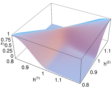
Figure 4: (Color online) From top to bottom, mean and variance of Loschmidt echo at size L=100𝐿100L=100. The region where the variance is large shrinks when increasing the system size L𝐿L. The height of the peak however remains constant.

Consider now a physical situation where an experimenter computes L¯¯subscript𝐿\overline{\mathcal{L}_{L}}. We inserted the labels T𝑇T and L𝐿L to stress that both size and expectation time are finite, as is required in a true experiment. Here we want to study the interplay between T𝑇T and L𝐿L. Consider first the case where we send L𝐿L to infinity, or more physically L𝐿L is the largest scale of our system. In this situation the spectrum of H𝐻H is practically continuous, and we can write the LE as

(t)𝑡\displaystyle\mathcal{L}\left(t\right) =\displaystyle= exp[L2π0πln(1sin2(ϑk(1)ϑk(2))sin2(Λk(2)t/2))𝑑k].𝐿2𝜋superscriptsubscript0𝜋1superscript2superscriptsubscriptitalic-ϑ𝑘1superscriptsubscriptitalic-ϑ𝑘2superscript2superscriptsubscriptΛ𝑘2𝑡2differential-d𝑘\displaystyle\exp\left[\frac{L}{2\pi}\int_{0}^{\pi}\ln\left(1-\sin^{2}\left(\vartheta_{k}^{(1)}-\vartheta_{k}^{\left(2\right)}\right)\sin^{2}\left(\Lambda_{k}^{\left(2\right)}t/2\right)\right)dk\right].
\displaystyle\equiv eLs(t)superscript𝑒𝐿𝑠𝑡\displaystyle e^{-Ls\left(t\right)}

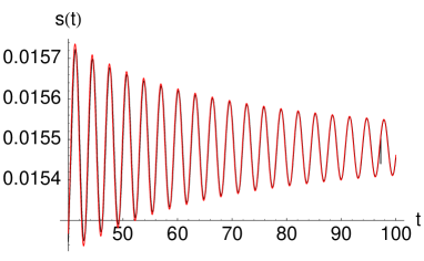
In this approximation we sent all the revival times to infinity and so the function (t)𝑡\mathcal{L}\left(t\right) is no longer almost periodic, but rather tends to a precise limit as t𝑡t\to\infty. We can calculate the limit s()𝑠s\left(\infty\right) and also the first corrections, as t𝑡t\to\infty. The procedure is outlined in the Appendix. The result is

s(t)=s()Am|t|3/2cos(tEm+34π)+(mM),s\left(t\right)=s\left(\infty\right)-\frac{A_{m}}{\left|t\right|^{3/2}}\cos\left(tE_{m}+\frac{3}{4}\pi\right)+\left(m\leftrightarrow M\right), (12)

where s()𝑠s\left(\infty\right) is the limiting value and Am/Msubscript𝐴𝑚𝑀A_{m/M} are constants which depend on h(i)superscript𝑖h^{\left(i\right)} and are given in the appendix. The result (29) has already been found in Silva (2008), here we provide the explicit form of the asymptotic value, s()𝑠s\left(\infty\right).

Since the function (t)=eLs(t)𝑡superscript𝑒𝐿𝑠𝑡\mathcal{L}\left(t\right)=e^{-Ls\left(t\right)} has a limit at infinity, its time average is precisely this limit ¯=eLs()¯superscript𝑒𝐿𝑠\overline{\mathcal{L}}=e^{-Ls\left(\infty\right)}. More precisely the distribution function becomes a delta function P(x)=δ(xeLs())𝑃𝑥𝛿𝑥superscript𝑒𝐿𝑠P\left(x\right)=\delta\left(x-e^{-Ls\left(\infty\right)}\right).

Consider now performing first the time average of Eq. (9). According to the discussion in section II.3, this requires at least observation times as large as TLmuch-greater-than𝑇𝐿T\gg L (if we are at criticality). The result in this case is (for the explicit computation see the following section)

¯=expk>0log(1sin2(ϑk(2)ϑk(1))/2)¯subscript𝑘01superscript2superscriptsubscriptitalic-ϑ𝑘2superscriptsubscriptitalic-ϑ𝑘12\overline{\mathcal{L}}=\exp\sum_{k>0}\log\left(1-\sin^{2}\left(\vartheta_{k}^{(2)}-\vartheta_{k}^{\left(1\right)}\right)/2\right) (13)

If now L𝐿L is large, we can approximate the sum with the integral: ¯=eLg(h(1),h(2))¯superscript𝑒𝐿𝑔superscript1superscript2\overline{\mathcal{L}}=e^{-Lg\left(h^{\left(1\right)},h^{\left(2\right)}\right)}. Calling δϑk=ϑk(2)ϑk(1)𝛿subscriptitalic-ϑ𝑘superscriptsubscriptitalic-ϑ𝑘2superscriptsubscriptitalic-ϑ𝑘1\delta\vartheta_{k}=\vartheta_{k}^{(2)}-\vartheta_{k}^{\left(1\right)} the two functions, g𝑔g and s()𝑠s\left(\infty\right) are given by

g𝑔\displaystyle g =\displaystyle= 12π0πln(1sin2(δϑk)/2)𝑑k,12𝜋superscriptsubscript0𝜋1superscript2𝛿subscriptitalic-ϑ𝑘2differential-d𝑘\displaystyle-\frac{1}{2\pi}\int_{0}^{\pi}\ln\left(1-\sin^{2}\left(\delta\vartheta_{k}\right)/2\right)dk, (14)
s()𝑠\displaystyle s\left(\infty\right) =\displaystyle= 1π0πln[(1+|cos(δϑk)|)/2]𝑑k.1𝜋superscriptsubscript0𝜋1𝛿subscriptitalic-ϑ𝑘2differential-d𝑘\displaystyle-\frac{1}{\pi}\int_{0}^{\pi}\ln\left[\left(1+\left|\cos\left(\delta\vartheta_{k}\right)\right|\right)/2\right]dk. (15)

We observed that the two averages eLgsuperscript𝑒𝐿𝑔e^{-Lg} – obtained by first doing the time average and then taking large L𝐿L – or eLs()superscript𝑒𝐿𝑠e^{-Ls\left(\infty\right)} – obtained by first considering L𝐿L large and then doing the time average – are qualitatively very similar for most values of the parameters h(i)superscript𝑖h^{\left(i\right)}. The only region where there is an appreciable difference is when h(1)superscript1h^{\left(1\right)} and h(2)superscript2h^{\left(2\right)} correspond to different phases (either |h(1)|<1superscript11\left|h^{\left(1\right)}\right|<1 and |h(2)|>1superscript21\left|h^{\left(2\right)}\right|>1 or vice-versa).

III.3 Moments of the Loschmidt echo in presence of degeneracy

Having the explicit form of the LE Eq. (9) we can compute its time average and also other moments. Since the Ising model is mapped to a free Fermi system on a finite lattice, and given the form of the quasi-particle dispersion ΛksubscriptΛ𝑘\Lambda_{k}, its spectrum is non-degenerate. In other words the Ising Hamiltonian is 1-non-degenerate. However, for the same reason, it is not k𝑘k-non-degenerate for k2𝑘2k\geq 2. This means that to compute moments higher than the first, we really need to use the explicit form Eq. (9) and cannot rely on the results of section II.3. For the first moment this problem does not arise, and we can either use ¯=npn2¯subscript𝑛superscriptsubscript𝑝𝑛2\overline{\mathcal{L}}=\sum_{n}p_{n}^{2} or do the time average of Eq. (9). Correctly the results coincide, and they rely on the fact that k(nkmk)Λk=0subscript𝑘subscript𝑛𝑘subscript𝑚𝑘subscriptΛ𝑘0\sum_{k}\left(n_{k}-m_{k}\right)\Lambda_{k}=0, implies nk=mksubscript𝑛𝑘subscript𝑚𝑘n_{k}=m_{k}, i.e. that the spectrum is non-degenerate. The result is

¯=k>0(1sin2(ϑk(1)ϑk(2))/2).¯subscriptproduct𝑘01superscript2superscriptsubscriptitalic-ϑ𝑘1superscriptsubscriptitalic-ϑ𝑘22\overline{\mathcal{L}}=\prod_{k>0}\left(1-\sin^{2}\left(\vartheta_{k}^{(1)}-\vartheta_{k}^{\left(2\right)}\right)/2\right). (16)

For later convenience we define αk=sin2(ϑk(1)ϑk(2))subscript𝛼𝑘superscript2superscriptsubscriptitalic-ϑ𝑘1superscriptsubscriptitalic-ϑ𝑘2\alpha_{k}=\sin^{2}\left(\vartheta_{k}^{(1)}-\vartheta_{k}^{\left(2\right)}\right). To compute higher moments we first rewrite Eq. (9) as

(t)𝑡\displaystyle\mathcal{L}\left(t\right) =\displaystyle= k>0(1+Xk(t)),subscriptproduct𝑘01subscript𝑋𝑘𝑡\displaystyle\prod_{k>0}\left(1+X_{k}\left(t\right)\right),
Xk(t)subscript𝑋𝑘𝑡\displaystyle X_{k}\left(t\right) =\displaystyle= αksin2(Λkt/2)=β=0,±1cβkeiβΛktsubscript𝛼𝑘superscript2subscriptΛ𝑘𝑡2subscript𝛽0plus-or-minus1superscriptsubscript𝑐𝛽𝑘superscript𝑒𝑖𝛽subscriptΛ𝑘𝑡\displaystyle-\alpha_{k}\sin^{2}\left(\Lambda_{k}t/2\right)=\sum_{\beta=0,\pm 1}c_{\beta}^{k}e^{i\beta\Lambda_{k}t}
c0k=αk2,c±1k=αk4.formulae-sequencesuperscriptsubscript𝑐0𝑘subscript𝛼𝑘2superscriptsubscript𝑐plus-or-minus1𝑘subscript𝛼𝑘4\displaystyle c_{0}^{k}=-\frac{\alpha_{k}}{2},\quad c_{\pm 1}^{k}=\frac{\alpha_{k}}{4}\,.

We write the n𝑛n-th power of the LE as

[(t)]nsuperscriptdelimited-[]𝑡𝑛\displaystyle\left[\mathcal{L}\left(t\right)\right]^{n} =\displaystyle= k>0(1+Yk(n)(t)),subscriptproduct𝑘01superscriptsubscript𝑌𝑘𝑛𝑡\displaystyle\prod_{k>0}\left(1+Y_{k}^{\left(n\right)}\left(t\right)\right),
Yk(n)(t)superscriptsubscript𝑌𝑘𝑛𝑡\displaystyle Y_{k}^{\left(n\right)}\left(t\right) =\displaystyle= m=1n(nm)[Xk(t)]mγ=0,±1,,±mgγ,k(n)eiγΛkt.superscriptsubscript𝑚1𝑛𝑛𝑚superscriptdelimited-[]subscript𝑋𝑘𝑡𝑚subscript𝛾0plus-or-minus1plus-or-minus𝑚superscriptsubscript𝑔𝛾𝑘𝑛superscript𝑒𝑖𝛾subscriptΛ𝑘𝑡\displaystyle\sum_{m=1}^{n}\left(\begin{array}[]{c}n\\ m\end{array}\right)\left[X_{k}\left(t\right)\right]^{m}\equiv\sum_{\gamma=0,\pm 1,\cdots,\pm m}g_{\gamma,k}^{\left(n\right)}e^{i\gamma\Lambda_{k}t}.

Now, when computing M𝑀M products of Yk(n)superscriptsubscript𝑌𝑘𝑛Y_{k}^{\left(n\right)} terms, only the γ=0𝛾0\gamma=0 term will survive after taking the time average. In other words:

Yk1(n)YkM(n)¯=g0,k1(n)g0,kM(n)¯superscriptsubscript𝑌subscript𝑘1𝑛superscriptsubscript𝑌subscript𝑘𝑀𝑛superscriptsubscript𝑔0subscript𝑘1𝑛superscriptsubscript𝑔0subscript𝑘𝑀𝑛\overline{Y_{k_{1}}^{\left(n\right)}\cdots Y_{k_{M}}^{\left(n\right)}}=g_{0,k_{1}}^{\left(n\right)}\cdots g_{0,k_{M}}^{\left(n\right)}

and so we have

[(t)]n¯=k>0(1+g0,k(n)).¯superscriptdelimited-[]𝑡𝑛subscriptproduct𝑘01superscriptsubscript𝑔0𝑘𝑛\overline{\left[\mathcal{L}\left(t\right)\right]^{n}}=\prod_{k>0}\left(1+g_{0,k}^{\left(n\right)}\right).

An explicit formula for g0,k(n)superscriptsubscript𝑔0𝑘𝑛g_{0,k}^{\left(n\right)} is

g0,k(n)=m=1n(nm)βi=0β1,βmcβ1kcβmk.superscriptsubscript𝑔0𝑘𝑛superscriptsubscript𝑚1𝑛𝑛𝑚subscriptsuperscriptsubscript𝛽𝑖0subscript𝛽1subscript𝛽𝑚superscriptsubscript𝑐subscript𝛽1𝑘superscriptsubscript𝑐subscript𝛽𝑚𝑘g_{0,k}^{\left(n\right)}=\sum_{m=1}^{n}\left(\begin{array}[]{c}n\\ m\end{array}\right)\sum_{\stackrel{{\scriptstyle\beta_{1},\ldots\beta_{m}}}{{\sum\beta_{i}=0}}}c_{\beta_{1}}^{k}\cdots c_{\beta_{m}}^{k}.

Noting that

βi=0β1,βmcβ1kcβmk=n1n0+2n1=mm!(n1!)2n0!(c0k)n0(c1k)2n1,subscriptsuperscriptsubscript𝛽𝑖0subscript𝛽1subscript𝛽𝑚superscriptsubscript𝑐subscript𝛽1𝑘superscriptsubscript𝑐subscript𝛽𝑚𝑘subscriptsubscript𝑛1subscript𝑛02subscript𝑛1𝑚𝑚superscriptsubscript𝑛12subscript𝑛0superscriptsuperscriptsubscript𝑐0𝑘subscript𝑛0superscriptsuperscriptsubscript𝑐1𝑘2subscript𝑛1\sum_{\stackrel{{\scriptstyle\beta_{1},\ldots\beta_{m}}}{{\sum\beta_{i}=0}}}c_{\beta_{1}}^{k}\cdots c_{\beta_{m}}^{k}=\sum_{\begin{subarray}{c}n_{1}\\ n_{0}+2n_{1}=m\end{subarray}}\frac{m!}{\left(n_{1}!\right)^{2}n_{0}!}\left(c_{0}^{k}\right)^{n_{0}}\left(c_{1}^{k}\right)^{2n_{1}},

we obtain

g0,k(n)superscriptsubscript𝑔0𝑘𝑛\displaystyle g_{0,k}^{\left(n\right)} =\displaystyle= m=1n(αk4)m(nm)tm(2tt21)m|t=0m!superscriptsubscript𝑚1𝑛superscriptsubscript𝛼𝑘4𝑚𝑛𝑚evaluated-atsuperscriptsubscript𝑡𝑚superscript2𝑡superscript𝑡21𝑚𝑡0𝑚\displaystyle\sum_{m=1}^{n}\left(\frac{-\alpha_{k}}{4}\right)^{m}\left(\begin{array}[]{c}n\\ m\end{array}\right)\frac{\left.\partial_{t}^{m}\left(2t-t^{2}-1\right)^{m}\right|_{t=0}}{m!}
=\displaystyle= m=1n(αk4)m(nm)(2mm).superscriptsubscript𝑚1𝑛superscriptsubscript𝛼𝑘4𝑚𝑛𝑚2𝑚𝑚\displaystyle\sum_{m=1}^{n}\left(\frac{-\alpha_{k}}{4}\right)^{m}\left(\begin{array}[]{c}n\\ m\end{array}\right)\left(\begin{array}[]{c}2m\\ m\end{array}\right).

For example we have

g0,k(1)superscriptsubscript𝑔0𝑘1\displaystyle g_{0,k}^{\left(1\right)} =\displaystyle= αk2subscript𝛼𝑘2\displaystyle-\frac{\alpha_{k}}{2}
g0,k(2)superscriptsubscript𝑔0𝑘2\displaystyle g_{0,k}^{\left(2\right)} =\displaystyle= αk+38αk2subscript𝛼𝑘38superscriptsubscript𝛼𝑘2\displaystyle-\alpha_{k}+\frac{3}{8}\alpha_{k}^{2}
g0,k(3)superscriptsubscript𝑔0𝑘3\displaystyle g_{0,k}^{\left(3\right)} =\displaystyle= 32αk+98αk2516αk332subscript𝛼𝑘98superscriptsubscript𝛼𝑘2516superscriptsubscript𝛼𝑘3\displaystyle-\frac{3}{2}\alpha_{k}+\frac{9}{8}\alpha_{k}^{2}-\frac{5}{16}\alpha_{k}^{3}
g0,k(4)superscriptsubscript𝑔0𝑘4\displaystyle g_{0,k}^{\left(4\right)} =\displaystyle= 2αk+94αk254αk3+35128αk4.2subscript𝛼𝑘94superscriptsubscript𝛼𝑘254superscriptsubscript𝛼𝑘335128superscriptsubscript𝛼𝑘4\displaystyle-2\alpha_{k}+\frac{9}{4}\alpha_{k}^{2}-\frac{5}{4}\alpha_{k}^{3}+\frac{35}{128}\alpha_{k}^{4}.

The variance of the LE is then given by

Δ2¯=k>0(1αk+38αk2)k>0(1αk+14αk2).¯Δsuperscript2subscriptproduct𝑘01subscript𝛼𝑘38superscriptsubscript𝛼𝑘2subscriptproduct𝑘01subscript𝛼𝑘14superscriptsubscript𝛼𝑘2\overline{\Delta\mathcal{L}^{2}}=\prod_{k>0}\left(1-\alpha_{k}+\frac{3}{8}\alpha_{k}^{2}\right)-\prod_{k>0}\left(1-\alpha_{k}+\frac{1}{4}\alpha_{k}^{2}\right). (20)

The first moment and the variance are plotted in figure 4. One should note that close to the critical points hc=±1subscript𝑐plus-or-minus1h_{c}=\pm 1 there appears a small region δh𝛿\delta h where the variance is large.

Equation (20) gives explicitly the variance in a case where the non-resonant hypothesis is violated. Since |αk|1subscript𝛼𝑘1\left|\alpha_{k}\right|\leq 1 generally the variance is given by the difference between two exponentially small quantities and so, a fortiori, is exponentially small in the system size L𝐿L. However, looking at figure 4 one notes a small region of parameter close to the critical points, where the variance is large. As we will see this fact has important consequences.

It is now interesting to compare the result in equation (20) with what would have been obtained assuming a non-resonant condition. Clearly the second moment computed assuming non resonance has less terms than the correct one. Since for the LE all the contributions are positive, the non-resonant result ought to be smaller. In other words, for the variance we must have Δ2¯Δnr2¯¯Δsuperscript2¯Δsuperscriptsubscriptnr2\overline{\Delta\mathcal{L}^{2}}\geq\overline{\Delta\mathcal{L}_{\mathrm{nr}}^{2}}.

Comparison with the non-resonant result

To compute the variance assuming non-resonance we use

nr2¯¯superscriptsubscriptnr2\displaystyle\overline{\mathcal{L}_{\mathrm{nr}}^{2}} =\displaystyle= ¯2+2i<jpi2pj2superscript¯22subscript𝑖𝑗superscriptsubscript𝑝𝑖2superscriptsubscript𝑝𝑗2\displaystyle\overline{\mathcal{L}}^{2}+2\sum_{i<j}p_{i}^{2}p_{j}^{2}
=\displaystyle= 2¯2ipi42superscript¯2subscript𝑖superscriptsubscript𝑝𝑖4\displaystyle 2\overline{\mathcal{L}}^{2}-\sum_{i}p_{i}^{4}

Using this formula together with Eq. (11) we obtain

Δnr2¯¯Δsuperscriptsubscriptnr2\displaystyle\overline{\Delta\mathcal{L}_{\mathrm{nr}}^{2}} =\displaystyle= ¯2k>0(1αk+18αk2)superscript¯2subscriptproduct𝑘01subscript𝛼𝑘18superscriptsubscript𝛼𝑘2\displaystyle\overline{\mathcal{L}}^{2}-\prod_{k>0}\left(1-\alpha_{k}+\frac{1}{8}\alpha_{k}^{2}\right)
=\displaystyle= k>0(1αk+14αk2)k>0(1αk+18αk2).subscriptproduct𝑘01subscript𝛼𝑘14superscriptsubscript𝛼𝑘2subscriptproduct𝑘01subscript𝛼𝑘18superscriptsubscript𝛼𝑘2\displaystyle\prod_{k>0}\left(1-\alpha_{k}+\frac{1}{4}\alpha_{k}^{2}\right)-\prod_{k>0}\left(1-\alpha_{k}+\frac{1}{8}\alpha_{k}^{2}\right).

We have verified that the inequality Δ2¯Δnr2¯¯Δsuperscript2¯Δsuperscriptsubscriptnr2\overline{\Delta\mathcal{L}^{2}}\geq\overline{\Delta\mathcal{L}_{\mathrm{nr}}^{2}} holds for all values of the coupling constants h(1)superscript1h^{\left(1\right)} and h(2)superscript2h^{\left(2\right)}. However the qualitative behavior of Δnr2¯¯Δsuperscriptsubscriptnr2\overline{\Delta\mathcal{L}_{\mathrm{nr}}^{2}} is very similar to the true variance Δ2¯¯Δsuperscript2\overline{\Delta\mathcal{L}^{2}}.

III.4 The Loschmidt echo distribution function

We now turn to consider the whole probability distribution of the LE. As we have noted earlier, for any L𝐿L finite being the spectrum discrete, (t)𝑡\mathcal{L}\left(t\right) is an almost periodic function. Actually (t)𝑡\mathcal{L}\left(t\right) belongs to a smaller class, since it is a trigonometric polynomial. In any case, most results we will present are valid for the larger class of almost periodic functions.

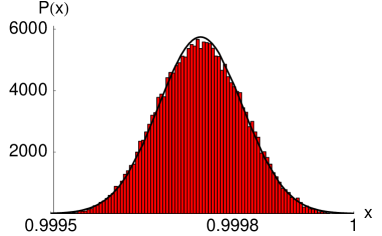
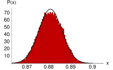
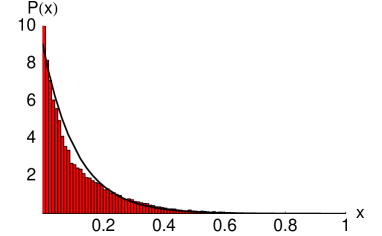
We now give the results for the whole LE probability distribution function. We have observed three kinds of universal behavior emerging in different, well defined regimes. i) Exponential behavior where the probability distribution is well approximated by ϑ(x)ex/¯/¯italic-ϑ𝑥superscript𝑒𝑥¯¯\vartheta\left(x\right)e^{-x/\overline{\mathcal{L}}}/\overline{\mathcal{L}} (figure 5), ii) Gaussian behavior, (figure 6), and iii) A universal double peaked, “batman-hood” shaped function, (figure 7). More precisely we have the following scenario:

  • δh𝛿\delta h large. In this case, for L𝐿L moderately large, the distribution is approximately exponential. The feature is more pronounced when h(1),h(2)superscript1superscript2h^{\left(1\right)},\,h^{\left(2\right)} are in different phases, the limiting case being h(1)±h(2)superscript1plus-or-minussuperscript2h^{\left(1\right)}\approx\pm h^{\left(2\right)}.

  • δh𝛿\delta h small. In this case we have to distinguish two situations:

    • h(i)superscript𝑖h^{\left(i\right)} close to the critical point:

      • *

        L|h(i)1|1ξmuch-less-than𝐿superscriptsuperscript𝑖11proportional-to𝜉L\ll\left|h^{\left(i\right)}-1\right|^{-1}\propto\xi, universal batman-hood distribution. Note that Lξmuch-less-than𝐿𝜉L\ll\xi is the so called quasi-critical regime.

      • *

        L|δh|1much-greater-than𝐿superscript𝛿1L\gg\left|\delta h\right|^{-1}, exponential distribution

    • Off critical:

      • *

        L|δh|2much-greater-than𝐿superscript𝛿2L\gg\left|\delta h\right|^{-2}, exponential distribution

      • *

        Otherwise Gaussian.

In other words, say that we fixed h(i)superscript𝑖h^{\left(i\right)} in order to have either a Gaussian or a double-peaked distribution. We can always find an L𝐿L large enough such that the distribution becomes exponential in both cases. However, for the Gaussian case we must reach considerably larger sizes L|δh|2much-greater-than𝐿superscript𝛿2L\gg\left|\delta h\right|^{-2} (compare figures 8 and 9).

We have observed an exponential distribution in the region of parameters where the average LE is much smaller than one: ¯1much-less-than¯1\overline{\mathcal{L}}\ll 1. Due to the bound 2¯<2¯2¯superscript22superscript¯2\overline{\mathcal{L}^{2}}<2\overline{\mathcal{L}}^{2}, one has Δ<¯2Δsuperscript¯2\Delta\mathcal{L}<\overline{\mathcal{L}}^{2} so that when ¯1much-less-than¯1\overline{\mathcal{L}}\ll 1 even the variance is small. Since the LE is supported in [0,1]01\left[0,1\right] and in particular (t)𝑡\mathcal{L}\left(t\right) must be positive we expect in the region ¯1much-less-than¯1\overline{\mathcal{L}}\ll 1 a distribution with positive support, with a large peak very close to zero, and rapidly decaying tail. We have verified that an exponential distribution of the form ϑ(x)ex/¯/¯italic-ϑ𝑥superscript𝑒𝑥¯¯\vartheta\left(x\right)e^{-x/\overline{\mathcal{L}}}/\overline{\mathcal{L}} gives a pretty good approximation in the region ¯1much-less-than¯1\overline{\mathcal{L}}\ll 1. Note in any case, that the exponential form is always an approximation. In particular, for x0𝑥0x\to 0 the true distribution P(x)𝑃𝑥P\left(x\right) tends to zero for any value of the parameters. This happens since we have always (t)>0𝑡0\mathcal{L}\left(t\right)>0 strictly. And so generally 0<min10subscriptmin10<\mathcal{L}_{\mathrm{min}}\leq\mathcal{L}\leq 1. This feature can be accounted for by adding a (small) ϵitalic-ϵ\epsilon term to the exponential: P(x)ex/¯ϵ/xproportional-to𝑃𝑥superscript𝑒𝑥¯italic-ϵ𝑥P\left(x\right)\propto e^{-x/\overline{\mathcal{L}}-\epsilon/x}.

Let us now investigate the conditions under which the first moment is small and so we expect an approximately exponential behavior. Looking at equation (13) we see that ¯1much-less-than¯1\overline{\mathcal{L}}\ll 1 holds when Lg(h(1),h(2))1much-greater-than𝐿𝑔superscript1superscript21Lg\left(h^{\left(1\right)},h^{\left(2\right)}\right)\gg 1 where g𝑔g is given by Eq. (14). Clearly the function g𝑔g is zero (its minimum) when h(1)=h(2)superscript1superscript2h^{\left(1\right)}=h^{\left(2\right)}, and is quadratic in the difference on the diagonal. Quite interestingly the function g𝑔g is appreciably different from zero only when h(1)superscript1h^{\left(1\right)} and h(2)superscript2h^{\left(2\right)} correspond to different phases (i.e. either |h(1)|<1superscript11\left|h^{\left(1\right)}\right|<1 and |h(2)|>1superscript21\left|h^{\left(2\right)}\right|>1 or vice-versa) so that in these cases we observe exponential behavior even for moderately small lattices. When h(1)superscript1h^{\left(1\right)} is close to h(2)superscript2h^{\left(2\right)}, but away from critical points, the function g𝑔g is quadratic in the difference δh𝛿\delta h so that ¯exp(const.×Lδh2)\overline{\mathcal{L}}\approx\exp\left(-\mathrm{const.}\times L\delta h^{2}\right). Hence to have ¯1much-less-than¯1\overline{\mathcal{L}}\ll 1 and so to observe approximate exponential behavior we obtain the relation Lδh2much-greater-than𝐿𝛿superscript2L\gg\delta h^{-2}. At criticality and for δh𝛿\delta h small instead, we can use ¯F4¯superscript𝐹4\overline{\mathcal{L}}\approx F^{4} where F𝐹F is the fidelity which scales as (see section II.2 and ref. Campos Venuti and Zanardi (2007)) . In the quantum Ising model we are considering we have d=ζ=ν=Δ=1𝑑𝜁𝜈Δ1d=\zeta=\nu=\Delta=1 and so the average behaves as ¯exp(const.×L2δh2)\overline{\mathcal{L}}\approx\exp\left(-\mathrm{const.}\times L^{2}\delta h^{2}\right). This means that for δh𝛿\delta h small around a critical point hc=±1subscript𝑐plus-or-minus1h_{c}=\pm 1, the condition to have an exponential distribution becomes Lδh1.much-greater-than𝐿𝛿superscript1L\gg\delta h^{-1}.

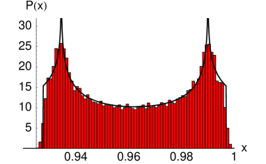
We now turn to consider the origin of the batman-hood shaped distribution function. As we have already noticed, the LE is a (finite) sum of cosines with given frequencies and amplitude. We can imagine a situation where only few frequencies contribute to the LE. In the limiting case, only two non-zero terms. That means that the LE can be approximated by

(t)=¯+Acos(ωAt)+Bcos(ωBt).𝑡¯𝐴subscript𝜔𝐴𝑡𝐵subscript𝜔𝐵𝑡\mathcal{L}\left(t\right)=\overline{\mathcal{L}}+A\cos\left(\omega_{A}t\right)+B\cos\left(\omega_{B}t\right). (21)

where we can assume A,B𝐴𝐵A,\,B positive.

We have devoted some attention to the probability distribution generated by such a function. If ωAsubscript𝜔𝐴\omega_{A} and ωBsubscript𝜔𝐵\omega_{B} are rationally dependent, the function is periodic and the distribution function has square root singularities at all values of \mathcal{L} where t(t)=0subscript𝑡𝑡0\partial_{t}\mathcal{L}\left(t\right)=0. However in our case the frequencies ωA/Bsubscript𝜔𝐴𝐵\omega_{A/B} are always rationally independent. In this case the vector 𝒙(t)=(ωAt,ωBt)𝒙𝑡subscript𝜔𝐴𝑡subscript𝜔𝐵𝑡\boldsymbol{x}\left(t\right)=\left(\omega_{A}t,\omega_{B}t\right) wraps around the torus in a uniform way. We can then invoke ergodicity and transform the time average into a “phase space” average (in this case the phase space is 𝒙=(x1,x2)𝒙subscript𝑥1subscript𝑥2\boldsymbol{x}=\left(x_{1},x_{2}\right)). Hence the probability distribution function is given by

P((t)=χ)𝑃𝑡𝜒\displaystyle P\left(\mathcal{L}\left(t\right)=\chi\right) =1(2π)202π𝑑x102π𝑑x2δ((x1,x2)χ).absent1superscript2𝜋2superscriptsubscript02𝜋differential-dsubscript𝑥1superscriptsubscript02𝜋differential-dsubscript𝑥2𝛿subscript𝑥1subscript𝑥2𝜒\displaystyle=\frac{1}{\left(2\pi\right)^{2}}\int_{0}^{2\pi}dx_{1}\int_{0}^{2\pi}dx_{2}\delta\left(\mathcal{L}\left(x_{1},x_{2}\right)-\chi\right).

By using Eq. (21) this probability density can be written as

P(χ+¯)=1π2Amax{1,(χB)A}min{1,(χ+B)A}dz(χ+BAz)(zχBA)(1z2).𝑃𝜒¯1superscript𝜋2𝐴superscriptsubscript1𝜒𝐵𝐴1𝜒𝐵𝐴𝑑𝑧𝜒𝐵𝐴𝑧𝑧𝜒𝐵𝐴1superscript𝑧2P\left(\chi+\overline{\mathcal{L}}\right)=\frac{1}{\pi^{2}A}\int_{\max\left\{-1,\frac{\left(\chi-B\right)}{A}\right\}}^{\min\left\{1,\frac{\left(\chi+B\right)}{A}\right\}}\frac{dz}{\sqrt{\left(\frac{\chi+B}{A}-z\right)\left(z-\frac{\chi-B}{A}\right)\left(1-z^{2}\right)}}. (22)

The integral above can be expressed in terms of elliptic functions, but we won’t need its explicit expression. Typically the function (22) is batman-hood shaped function (see fig. 7), with support in [¯|A+B|,¯+|A+B|]¯𝐴𝐵¯𝐴𝐵\left[\overline{\mathcal{L}}-\left|A+B\right|,\overline{\mathcal{L}}+\left|A+B\right|\right] and two peaks at χ=¯±|AB|𝜒plus-or-minus¯𝐴𝐵\chi=\overline{\mathcal{L}}\pm\left|A-B\right|. The divergence at the peaks position is of logarithmic type, close to the peaks (i.e. χ=¯±|AB|+ϵ𝜒plus-or-minus¯𝐴𝐵italic-ϵ\chi=\overline{\mathcal{L}}\pm\left|A-B\right|+\epsilon) one has

P(χ)=ln(ϵ)2π2|AB|+O(1).𝑃𝜒italic-ϵ2superscript𝜋2𝐴𝐵𝑂1P\left(\chi\right)=-\frac{\ln\left(\epsilon\right)}{2\pi^{2}\sqrt{\left|AB\right|}}+O\left(1\right).

Note that we never observe the limiting case where B=0𝐵0B=0 and (t)𝑡\mathcal{L}\left(t\right) becomes a periodic function. This means that even a very small spectral weight on B𝐵B cannot be discarded. On the other hand the distribution function (22) seems to be quite stable against the presence of other oscillating terms with small spectral weight. This stability can be seen in fig. 7 where one clearly has at least three frequencies with reasonable spectral weight, but the probability density is still well approximated by a batman-hood.
Refer to caption
Refer to caption
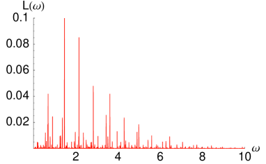
Figure 5: (Color online) Approximate exponential behavior. Parameters are L=18,h(1)=0.3,h(2)=1.4formulae-sequence𝐿18formulae-sequencesuperscript10.3superscript21.4L=18,\,h^{(1)}=0.3,\,h^{(2)}=1.4. When δh𝛿\delta h is large this behavior is observed even for moderate sizes (here L=18𝐿18L=18), (upper panel). The thick line reproduces ϑ(x)ex/¯/¯italic-ϑ𝑥superscript𝑒𝑥¯¯\vartheta\left(x\right)e^{-x/\overline{\mathcal{L}}}/\overline{\mathcal{L}} with ¯¯\overline{\mathcal{L}} given by equation (16). In the lower panel we plot the Fourier series ^disc(ω)subscript^disc𝜔\hat{\mathcal{L}}_{\mathrm{disc}}\left(\omega\right) given by Eq. (23).
Refer to caption
Refer to caption
Figure 6: (Color online) Gaussian behavior for δh𝛿\delta h small but away from criticality. Parameters are L=20,h(1)=0.1,h(2)=0.11formulae-sequence𝐿20formulae-sequencesuperscript10.1superscript20.11L=20,\,h^{(1)}=0.1,\,h^{(2)}=0.11. Note that the distribution function is an extremely peaked Gaussian (upper panel). The thick line is a Gaussian with mean and variance given by Eqns. (16) and (20). In the bottom panel one can notice that many frequencies contribute to the LE. The one particle contribution c(ω)𝑐𝜔c\left(\omega\right), Eq. (25), is given by the black dots while the red curve gives the true spectral decomposition ^disc(ω)subscript^disc𝜔\hat{\mathcal{L}}_{\mathrm{disc}}\left(\omega\right) given by Eq. (23).
Refer to caption
Refer to caption
Figure 7: (Color online) Typical “batman-hood” behavior. Parameters are L=40,h(1)=0.99,h(2)=1.01formulae-sequence𝐿40formulae-sequencesuperscript10.99superscript21.01L=40,\,h^{(1)}=0.99,\,h^{(2)}=1.01. Upper panel: probability distribution (histogram) together with the result of the approximation given in Eq. 21 (thick line). The mean ¯¯\overline{\mathcal{L}} is taken from Eq. (9) while the parameters A𝐴A and B𝐵B are obtained by computing the two largest spectral weights (see equation (24)). Lower panel: the red curve is the Fourier series ^disc(ω)subscript^disc𝜔\hat{\mathcal{L}}_{\mathrm{disc}}\left(\omega\right) (projected spectral density), black curve shows the highest coefficient c(ω)𝑐𝜔c\left(\omega\right) given by Eq. (25), together with allowed frequencies (black dots).

Spectral analysis

To understand the behavior of P(=x)𝑃𝑥P\left(\mathcal{L}=x\right) we do a spectral analysis of (t)𝑡\mathcal{L}\left(t\right) to see which frequencies contribute most. In fact, for almost periodic functions there is a similar Fourier decomposition as for periodic functions. The Fourier expansion is given in this case by ^disc(ω)=(t)eiωt¯subscript^disc𝜔¯𝑡superscript𝑒𝑖𝜔𝑡\hat{\mathcal{L}}_{\mathrm{disc}}\left(\omega\right)=\overline{\mathcal{L}\left(t\right)e^{i\omega t}}. Taking into account Eq. (8) ^disc(ω)subscript^disc𝜔\hat{\mathcal{L}}_{\mathrm{disc}}\left(\omega\right) can be written as

^disc(ω)=n,mpnpmδω,EnEmsubscript^disc𝜔subscript𝑛𝑚subscript𝑝𝑛subscript𝑝𝑚subscript𝛿𝜔subscript𝐸𝑛subscript𝐸𝑚\hat{\mathcal{L}}_{\mathrm{disc}}\left(\omega\right)=\sum_{n,m}p_{n}p_{m}\delta_{\omega,E_{n}-E_{m}} (23)

We would like to know which frequencies have the largest weight. This is achieved by expanding the product in Eq. (9) 444A more precise approximation valid also in region where δh𝛿\delta h is large, is given by (t)=k>0(1+c0k+X~k(t))¯(1+k>0(1+c0k)1X~k(t))𝑡subscriptproduct𝑘01superscriptsubscript𝑐0𝑘subscript~𝑋𝑘𝑡similar-to-or-equals¯1subscript𝑘0superscript1superscriptsubscript𝑐0𝑘1subscript~𝑋𝑘𝑡\mathcal{L}\left(t\right)=\prod_{k>0}\left(1+c_{0}^{k}+\tilde{X}_{k}\left(t\right)\right)\simeq\overline{\mathcal{L}}\left(1+\sum_{k>0}\left(1+c_{0}^{k}\right)^{-1}\tilde{X}_{k}\left(t\right)\right). The two expressions coincide when δh𝛿\delta h is small.

(t)𝑡\displaystyle\mathcal{L}\left(t\right) =\displaystyle= 1+k>0Xk(t)+k1,k2>0Xk1(t)Xk2(t)+1subscript𝑘0subscript𝑋𝑘𝑡subscriptsubscript𝑘1subscript𝑘20subscript𝑋subscript𝑘1𝑡subscript𝑋subscript𝑘2𝑡\displaystyle 1+\sum_{k>0}X_{k}\left(t\right)+\sum_{k_{1},k_{2}>0}X_{k_{1}}\left(t\right)X_{k_{2}}\left(t\right)+\cdots
=\displaystyle= ¯+k>0X~k(t)+k1,k2>0X~k1(t)X~k2(t)+¯subscript𝑘0subscript~𝑋𝑘𝑡subscriptsubscript𝑘1subscript𝑘20subscript~𝑋subscript𝑘1𝑡subscript~𝑋subscript𝑘2𝑡\displaystyle\overline{\mathcal{L}}+\sum_{k>0}\tilde{X}_{k}\left(t\right)+\sum_{k_{1},k_{2}>0}\tilde{X}_{k_{1}}\left(t\right)\tilde{X}_{k_{2}}\left(t\right)+\cdots
withwith\displaystyle\mathrm{with} X~k(t)=β=±1cβkeiβΛkt=αk2cos(Λkt).subscript~𝑋𝑘𝑡subscript𝛽plus-or-minus1superscriptsubscript𝑐𝛽𝑘superscript𝑒𝑖𝛽subscriptΛ𝑘𝑡subscript𝛼𝑘2subscriptΛ𝑘𝑡\displaystyle\tilde{X}_{k}\left(t\right)=\sum_{\beta=\pm 1}c_{\beta}^{k}e^{i\beta\Lambda_{k}t}=\frac{\alpha_{k}}{2}\cos\left(\Lambda_{k}t\right).

Now, since each X~k(t)subscript~𝑋𝑘𝑡\tilde{X}_{k}\left(t\right) is smaller than 1/2121/2 in modulus, it is reasonable to approximate the LE with the first two terms of this expansion and we obtain

(t)¯+k>0αk2cos(Λkt).similar-to-or-equals𝑡¯subscript𝑘0subscript𝛼𝑘2subscriptΛ𝑘𝑡\mathcal{L}\left(t\right)\simeq\overline{\mathcal{L}}+\sum_{k>0}\frac{\alpha_{k}}{2}\cos\left(\Lambda_{k}t\right). (24)

In this approximation we only wrote the zero-frequency contribution, which corresponds to the mean, and the contribution coming from the one particle spectrum. The next term has also contributions coming from the two particle spectrum. To be more precise, call E(n)superscript𝐸𝑛E^{\left(n\right)} the energy of the n𝑛n-particle spectrum then Ea(1)Eb(0)Λkproportional-tosuperscriptsubscript𝐸𝑎1superscriptsubscript𝐸𝑏0subscriptΛ𝑘E_{a}^{\left(1\right)}-E_{b}^{\left(0\right)}\propto\Lambda_{k}, (first order contribution), while Ea(1)Eb(1)Λk1Λk2proportional-tosuperscriptsubscript𝐸𝑎1superscriptsubscript𝐸𝑏1subscriptΛsubscript𝑘1subscriptΛsubscript𝑘2E_{a}^{\left(1\right)}-E_{b}^{\left(1\right)}\propto\Lambda_{k_{1}}-\Lambda_{k_{2}}, and Ea(2)Eb(0)Λk1+Λk2proportional-tosuperscriptsubscript𝐸𝑎2superscriptsubscript𝐸𝑏0subscriptΛsubscript𝑘1subscriptΛsubscript𝑘2E_{a}^{\left(2\right)}-E_{b}^{\left(0\right)}\propto\Lambda_{k_{1}}+\Lambda_{k_{2}}(second order contribution with less spectral weight).

Note that we expect Eq. (24) to be approximately valid (with a different form for the amplitudes and the frequencies) also for non integrable models in which a one-particle approximation works well.

Now, if there is a regime where the amplitudes αk/2subscript𝛼𝑘2\alpha_{k}/2 are highly peaked around few quasi-momenta, in the limiting case only two, then the LE can be approximated as in Eq. (21) and we expect a double peaked distribution function. So we are led to study the (one-particle) amplitude function

c(ω)αk2|ω=Λk,ω[Em,EM].formulae-sequence𝑐𝜔evaluated-atsubscript𝛼𝑘2𝜔subscriptΛ𝑘𝜔subscript𝐸𝑚subscript𝐸𝑀c\left(\omega\right)\equiv\left.\frac{\alpha_{k}}{2}\right|_{\omega=\Lambda_{k}},\,\,\omega\in\left[E_{m},E_{M}\right]. (25)

Generally c(ω)𝑐𝜔c\left(\omega\right) is a bell-shaped function, starting linearly from the band minimum Emsubscript𝐸𝑚E_{m}, reaching a maximum value and then decreasing to zero at the band maximum EMsubscript𝐸𝑀E_{M}. It is not difficult to show that not (a), when δh𝛿\delta h is small and for roughly |1h(2)|101less-than-or-similar-to1superscript2superscript101\left|1-h^{(2)}\right|\lesssim 10^{-1}, c(ω)𝑐𝜔c\left(\omega\right) starts developing a peak, the width of which being proportional to |1h(2)|1superscript2\left|1-h^{(2)}\right|. In the limiting case h(2)=1superscript21h^{(2)}=1, c(ω)𝑐𝜔c\left(\omega\right) has its maximum at Em=0subscript𝐸𝑚0E_{m}=0 and then decreases monotonically to EM=2subscript𝐸𝑀2E_{M}=2. So, for δh𝛿\delta h small and for |1h(2)|101less-than-or-similar-to1superscript2superscript101\left|1-h^{(2)}\right|\lesssim 10^{-1}, c(ω)𝑐𝜔c\left(\omega\right) is a peaked function. In order to have few frequencies fall within the peak, and so to have large spectral weight on few frequencies, we must additionally have L|1h(2)|1much-less-than𝐿1superscript21L\left|1-h^{(2)}\right|\ll 1. This is easily seen analyzing the dispersion ΛksubscriptΛ𝑘\Lambda_{k} for h(2)superscript2h^{(2)} close to the critical point not (b). All in all, the conditions to have a batman-hood distribution, are δh𝛿\delta h small and L|1h(2)|1much-less-than𝐿1superscript21L\left|1-h^{(2)}\right|\ll 1. The feature is more pronounced when the hisubscript𝑖h_{i} are not precisely critical. In fact even though c(ω)𝑐𝜔c\left(\omega\right) is most peaked when h(2)=1superscript21h^{(2)}=1 (and the peak is at ω=0𝜔0\omega=0), we have to remember that the allowed values of ω𝜔\omega are ωn=Λknsubscript𝜔𝑛subscriptΛsubscript𝑘𝑛\omega_{n}=\Lambda_{k_{n}} where kn=π(2n+1)/Lsubscript𝑘𝑛𝜋2𝑛1𝐿k_{n}=\pi\left(2n+1\right)/L, and the smallest frequency is ω1=Λπ/Lsubscript𝜔1subscriptΛ𝜋𝐿\omega_{1}=\Lambda_{\pi/L}. If we perturb h(2)superscript2h^{(2)} from 1 the peak of c(ω)𝑐𝜔c\left(\omega\right) shifts to the right, approaching ω1subscript𝜔1\omega_{1}, so it is favorable to have h(2)1superscript21h^{(2)}\neq 1. Not surprisingly, the conditions to have a batman-hood probability density, coincide with having a large variance (see figure 4 bottom panel).

Generally fixing h(i)superscript𝑖h^{\left(i\right)} and increasing the size L𝐿L, one eventually violates the quasi-critical condition Lξmuch-less-than𝐿𝜉L\ll\xi. At this stage the double-peak feature tends to disappear and the distribution approaches an exponential one. This can be clearly seen in figure 8. From this figure one can have the impression that the “double-peak feature” is a prerequisite of short sizes, since in this case one has few frequencies anyway. As we have tried to explain instead, this feature survives for larger sizes, provided we shrink δh𝛿\delta h sufficiently (figure 7).

Instead, when δh𝛿\delta h is small but h(i)superscript𝑖h^{\left(i\right)} are far from the critical point, then c(ω)𝑐𝜔c\left(\omega\right) is not peaked, and many frequencies have a large spectral weight (see figure 6). In this case the distribution becomes Gaussian.The emergence of a Gaussian distribution can be qualitatively understood in the following way. First write the LE according to its spectral decomposition (t)=nAneitωn𝑡subscript𝑛subscript𝐴𝑛superscript𝑒𝑖𝑡subscript𝜔𝑛\mathcal{L}\left(t\right)=\sum_{n}A_{n}e^{it\omega_{n}} where the amplitudes are precisely given by An=^disc(ωn)subscript𝐴𝑛subscript^discsubscript𝜔𝑛A_{n}=\hat{\mathcal{L}}_{\mathrm{disc}}\left(\omega_{n}\right) and are positive. When the frequencies are rationally independent the variables xn=tωnsubscript𝑥𝑛𝑡subscript𝜔𝑛x_{n}=t\omega_{n} wrap uniformly around a large dimensional torus. Then one can consider each An×etxnsubscript𝐴𝑛superscript𝑒𝑡subscript𝑥𝑛A_{n}\times e^{tx_{n}} as an independent random variable. The assumption δh𝛿\delta h is small but h(i)superscript𝑖h^{\left(i\right)} away from criticality corresponds to say that (t)𝑡\mathcal{L}\left(t\right) can be considered as a sum of many independent random variables, giving rise to a Gaussian distribution. When L|δh|2much-greater-than𝐿superscript𝛿2L\gg\left|\delta h\right|^{-2} the conditions of independence breaks down and we recover an approximate exponential behavior.
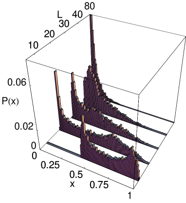
Refer to caption
Figure 8: (Color online) Batman-hood distribution approaching an exponential one when increasing system size L𝐿L at fixed h(i)superscript𝑖h^{\left(i\right)}. Parameters are h(1)=0.9,h(2)=1.2formulae-sequencesuperscript10.9superscript21.2h^{(1)}=0.9,\,h^{(2)}=1.2 and chain length are L=10,20,30,40𝐿10203040L=10,20,30,40.
Refer to caption
Figure 9: (Color online) Gaussian distribution approaching an exponential one when increasing system size L𝐿L at fixed h(i)superscript𝑖h^{\left(i\right)}. Parameters are h(1)=0.2,h(2)=0.6formulae-sequencesuperscript10.2superscript20.6h^{(1)}=0.2,\,h^{(2)}=0.6 and chain length are L=20,30,40,80,120𝐿20304080120L=20,30,40,80,120.

IV Probability distribution function for the magnetization

In the same spirit we can compute the probability distribution of a local operator. The first candidate that comes to mind is the transverse magnetization. We computed the following time dependent observable m(t)=ψ(1)|eitH(2)σizeitH(2)|ψ(1)𝑚𝑡quantum-operator-productsuperscript𝜓1superscript𝑒𝑖𝑡superscript𝐻2superscriptsubscript𝜎𝑖𝑧superscript𝑒𝑖𝑡superscript𝐻2superscript𝜓1m\left(t\right)=\left\langle\psi^{\left(1\right)}|e^{itH^{\left(2\right)}}\sigma_{i}^{z}e^{-itH^{\left(2\right)}}|\psi^{\left(1\right)}\right\rangle. Using again equation (10) one obtains 555This is precisely Eq. (5.6) of Barouch et al. (1970) in the zero temperature limit.

m(t)=1Lkcos(ϑk(2))cos(δϑk)+sin(ϑk(2))sin(δϑk)cos(tΛk(2)),𝑚𝑡1𝐿subscript𝑘superscriptsubscriptitalic-ϑ𝑘2𝛿subscriptitalic-ϑ𝑘superscriptsubscriptitalic-ϑ𝑘2𝛿subscriptitalic-ϑ𝑘𝑡superscriptsubscriptΛ𝑘2m\left(t\right)=\frac{1}{L}\sum_{k}\cos\left(\vartheta_{k}^{\left(2\right)}\right)\cos\left(\delta\vartheta_{k}\right)+\sin\left(\vartheta_{k}^{\left(2\right)}\right)\sin\left(\delta\vartheta_{k}\right)\cos\left(t\Lambda_{k}^{\left(2\right)}\right), (26)

where the quasi-momenta range now in the whole Brillouine zone: k=π(2n+1)/L,𝑘𝜋2𝑛1𝐿k=\pi\left(2n+1\right)/L, n=0,1,,L1𝑛01𝐿1n=0,1,\ldots,L-1. Correctly, when h(1)=h(2)superscript1superscript2h^{\left(1\right)}=h^{\left(2\right)} we recover the zero temperature equilibrium result σiz=L1kcos(ϑk)delimited-⟨⟩superscriptsubscript𝜎𝑖𝑧superscript𝐿1subscript𝑘subscriptitalic-ϑ𝑘\langle\sigma_{i}^{z}\rangle=L^{-1}\sum_{k}\cos\left(\vartheta_{k}\right).

From equation (26) we see that m(t)𝑚𝑡m\left(t\right) can be written —exactly— as a constant term plus an an oscillating part with frequencies given by the single particle spectrum ΛksubscriptΛ𝑘\Lambda_{k}. The discussion on characteristic times becomes simplified as all time scales are uniquely determined by Λk(2)superscriptsubscriptΛ𝑘2\Lambda_{k}^{\left(2\right)}. For example the time T1subscript𝑇1T_{1} necessary to observe the correct mean: mT1¯=m¯¯superscript𝑚subscript𝑇1¯𝑚\overline{m^{T_{1}}}=\overline{m} must simply satisfy T1gap1much-greater-thansubscript𝑇1superscriptgap1T_{1}\gg\mathrm{gap}^{-1} which means T1Lmuch-greater-thansubscript𝑇1𝐿T_{1}\gg L in the quasi-critical regime |h(2)1|1Lmuch-greater-thansuperscriptsuperscript211𝐿\left|h^{\left(2\right)}-1\right|^{-1}\gg L, while it suffices to have T1O(1)much-greater-thansubscript𝑇1𝑂1T_{1}\gg O\left(1\right) away from criticality. Given equation (26) it is not difficult to compute the mean and the variance, which are given by

m¯¯𝑚\displaystyle\overline{m} =\displaystyle= 1Lkcos(ϑk(2))cos(δϑk)1𝐿subscript𝑘superscriptsubscriptitalic-ϑ𝑘2𝛿subscriptitalic-ϑ𝑘\displaystyle\frac{1}{L}\sum_{k}\cos\left(\vartheta_{k}^{\left(2\right)}\right)\cos\left(\delta\vartheta_{k}\right) (27)
Δm2¯¯Δsuperscript𝑚2\displaystyle\overline{\Delta m^{2}} =\displaystyle= 1L2ksin2(ϑk(2))sin2(δϑk).1superscript𝐿2subscript𝑘superscript2superscriptsubscriptitalic-ϑ𝑘2superscript2𝛿subscriptitalic-ϑ𝑘\displaystyle\frac{1}{L^{2}}\sum_{k}\sin^{2}\left(\vartheta_{k}^{\left(2\right)}\right)\sin^{2}\left(\delta\vartheta_{k}\right). (28)

Some comments are in order here. First fixing h(1),h(2)superscript1superscript2h^{\left(1\right)},\,h^{\left(2\right)} the variance (figure 10) goes to zero as L1superscript𝐿1L^{-1} and not exponentially fast as was the case for the LE. Second, the spectral weight associated to the frequency Λk(2)superscriptsubscriptΛ𝑘2\Lambda_{k}^{\left(2\right)} is sin(ϑk(2))sin(δϑk)superscriptsubscriptitalic-ϑ𝑘2𝛿subscriptitalic-ϑ𝑘\sin\left(\vartheta_{k}^{\left(2\right)}\right)\sin\left(\delta\vartheta_{k}\right). We observed that there are always many frequencies with large spectral weight. In other words the spectral weight function is never peaked.

These comments suggest us to expect a Gaussian behavior for the probability distribution function of the magnetization irrespective of the parameters approaching critical values. This has indeed been observed (fig. 11).
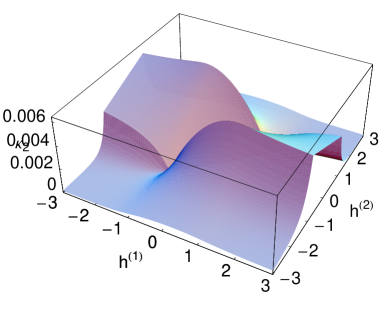
Refer to caption
Figure 10: (Color online) Variance of the magnetization as given by Eq. (10) for L=80𝐿80L=80. A signature of criticality are the cusps at h(2)=±1superscript2plus-or-minus1h^{\left(2\right)}=\pm 1.
Refer to caption
Figure 11: (Color online) The probability distribution for the magnetization has only Gaussian behavior. Here parameters are L=40,h(1)=0.9formulae-sequence𝐿40superscript10.9L=40,\,h^{\left(1\right)}=0.9, h(2)=1.01superscript21.01h^{\left(2\right)}=1.01. The continuous line is a Gaussian with mean and variance given by Eqns. (27) and (28).

V Conclusions

The unitary character of the dynamics of a closed quantum system implies that whatever relevant notion of equilibration one might have has to be a subtle one. In this paper we investigated the unitary equilibration of a quantum system after a sudden change of its Hamiltonian parameter. To this aim we used a prototypical time-dependent quantity: the Loschmidt echo. We established how the global features of \mathcal{L} depend on the physical properties of the initial state preparation and on those of the quench Hamiltonian. The central object of our analysis is given by the long time probability distribution for \mathcal{L}: P(x)=δ((t)x)¯:=limTT10Tδ((t)x)𝑑t𝑃𝑥¯𝛿𝑡𝑥assignsubscript𝑇superscript𝑇1superscriptsubscript0𝑇𝛿𝑡𝑥differential-d𝑡P(x)=\overline{\delta(\mathcal{L}(t)-x)}:=\lim_{T\to\infty}T^{-1}\int_{0}^{T}\delta\left(\mathcal{L}\left(t\right)-x\right)dt. Broadly speaking concentration phenomena for P𝑃P correspond to quantum equilibration.

Here below for the reader’s sake we summarize the main findings of the paper

  • Resorting to a cumulant expansion we characterized the ”short” time behavior of (t).𝑡\mathcal{L}(t). Different regimes can be identified depending on the most relevant scaling dimension of the quench Hamiltonian. When the central limit theorem (CLT) applies one has a Gaussian decay over a time scale O(1)𝑂1O(1) for gapped systems. For the critical case the time-scale becomes O(Lζ)𝑂superscript𝐿𝜁O\left(L^{\zeta}\right) in a small region |δh|L(d+ζΔ)much-less-than𝛿superscript𝐿𝑑𝜁Δ\left|\delta h\right|\ll L^{-\left(d+\zeta-\Delta\right)}. At critical points the CLT can be violated and (t)𝑡\mathcal{L}(t) takes a universal non-Gaussian form for sufficiently relevant perturbations.

  • We discussed the general structure of the higher momenta of P𝑃P i.e., μk:=k(t)¯=xkP(x)𝑑xassignsubscript𝜇𝑘¯superscript𝑘𝑡superscript𝑥𝑘𝑃𝑥differential-d𝑥\mu_{k}:=\overline{\mathcal{L}^{k}(t)}=\int x^{k}P(x)dx using the so-called non-resonant hypothesis. We showed that all the μksubscript𝜇𝑘\mu_{k} are bounded by those corresponding to a Poissonian distribution i.e., P(x)=ϑ(x)exp(x/¯)/¯𝑃𝑥italic-ϑ𝑥𝑥¯¯P(x)=\vartheta\left(x\right)\exp(-x/\overline{\mathcal{L}})/\overline{\mathcal{L}}.

  • Using exact results for the quantum Ising chain we rigorously analyzed the interplay between the chain length L𝐿L and the averaging time T.𝑇T. In particular we showed how the limit limTsubscript𝑇\lim_{T\to\infty} and the thermodynamical one i.e., limLsubscript𝐿\lim_{L\to\infty} do not commute. While in finite systems the (t)𝑡\mathcal{L}(t) is an almost-periodic function, in the thermodynamical limit :=limt(t)assignsubscriptsubscript𝑡𝑡\mathcal{L}_{\infty}:=\lim_{t\to\infty}\mathcal{L}(t) exists and P(x)δ(x)𝑃𝑥𝛿𝑥subscriptP(x)\rightarrow\delta(x-\mathcal{L}_{\infty}). We explicitly computed subscript\mathcal{L}_{\infty} and the way it is asymptotically approached for large t.𝑡t. We gave a general closed form for the exact μksubscript𝜇𝑘\mu_{k}’s and compared with that obtained with the non-resonant hypothesis

  • For the quantum Ising chain we numerically investigated P(x).𝑃𝑥P(x). We identified three universal regimes a) An exponential one (P𝑃P is Poissonian) when L𝐿L is the largest scale of the system b) A Gaussian one for intermediate L𝐿L and initial state and quench parameters close and off-critical c) A ”Batman-hood” shape for P𝑃P when the parameters are close to each other and close to criticality. This result holds in the quasi-critical region L|h(i)1|1,(i=1,2).much-less-than𝐿superscript𝑖11𝑖12L|h^{(i)}-1|\ll 1,\,(i=1,2).

  • Finally, for the sake of the comparison of the Loschmidt echo with a prototypical observable, we computed the time-dependent magnetization after the quench and studied its long-time statistics. In this case only a Gaussian regime appears to be reachable.

We have shown that the Loschmidt echo encodes sophisticated information about the quantum equilibration dynamics. For finite system vastly different time-scales arise: short time relaxation is intertwined with a complex a pattern of collapses and revivals and eventually Poincare recurrences. Unveiling how these phenomena depend on spectral properties of the underlying Hamiltonians, is one of the key challenges in the way to understand emergent thermal behavior in closed quantum systems.

Acknowledgements.
The authors gratefully acknowledge discussions with H. Saleur and A. Winter. Supported by NSF grants: PHY-803304,DMR-0804914 and European project COQUIT FP7-ICT-2007-C, n. 233747. LCV wishes to thank S. Fortunato, F. Radicchi and A. Lancichinetti for providing a result on the permutation group and D. Burgarth for useful discussions.

Appendix

Refer to caption
Figure 12: Typical behavior of the function s(t)𝑠𝑡s\left(t\right) (black line) in the thermodynamic limit. The red line is the approximation given by Eq. (29). Parameters are h(1)=1.3superscript11.3h^{(1)}=1.3, h(2)=2superscript22h^{(2)}=2.

Asymptotic of s(t)𝑠𝑡s\left(t\right)

Here we want to compute the asymptotic of s(t)𝑠𝑡s\left(t\right) for t𝑡t\to\infty, that is the integral:

s(t)=12π0πln(1sin2(ϑk(1)ϑk(2))sin2(Λk(2)t/2))𝑑k𝑠𝑡12𝜋superscriptsubscript0𝜋1superscript2superscriptsubscriptitalic-ϑ𝑘1superscriptsubscriptitalic-ϑ𝑘2superscript2superscriptsubscriptΛ𝑘2𝑡2differential-d𝑘s\left(t\right)=-\frac{1}{2\pi}\int_{0}^{\pi}\ln\left(1-\sin^{2}\left(\vartheta_{k}^{(1)}-\vartheta_{k}^{\left(2\right)}\right)\sin^{2}\left(\Lambda_{k}^{\left(2\right)}t/2\right)\right)dk

We can go to energy integration setting Λk(2)=ωsuperscriptsubscriptΛ𝑘2𝜔\Lambda_{k}^{\left(2\right)}=\omega

s(t)=12πEmEMln[1α(ω)sin2(ωt/2)]ρ(ω)𝑑ω.𝑠𝑡12𝜋superscriptsubscriptsubscript𝐸𝑚subscript𝐸𝑀1𝛼𝜔superscript2𝜔𝑡2𝜌𝜔differential-d𝜔s\left(t\right)=-\frac{1}{2\pi}\int_{E_{m}}^{E_{M}}\ln\left[1-\alpha\left(\omega\right)\sin^{2}\left(\omega t/2\right)\right]\rho\left(\omega\right)d\omega.

Where Em=2min{|1+h(2)|,|1h(2)|}subscript𝐸𝑚21superscript21superscript2E_{m}=2\min\left\{\left|1+h^{(2)}\right|,\left|1-h^{(2)}\right|\right\} and EM=2max{|1+h(2)|,|1h(2)|}subscript𝐸𝑀21superscript21superscript2E_{M}=2\max\left\{\left|1+h^{(2)}\right|,\left|1-h^{(2)}\right|\right\}. To be explicit:

ρ(ω)𝜌𝜔\displaystyle\rho\left(\omega\right) =\displaystyle= 2ω(ω2Em2)(EM2ω2)2𝜔superscript𝜔2superscriptsubscript𝐸𝑚2superscriptsubscript𝐸𝑀2superscript𝜔2\displaystyle\frac{2\omega}{\sqrt{\left(\omega^{2}-E_{m}^{2}\right)\left(E_{M}^{2}-\omega^{2}\right)}}
α(ω)𝛼𝜔\displaystyle\alpha\left(\omega\right) =\displaystyle= (ω2Em2)(EM2ω2)(h(2)h(1))24(h(2))2[4(h(2)h(1))(1h(1)h(2))+h(1)ω2]ω2.superscript𝜔2superscriptsubscript𝐸𝑚2superscriptsubscript𝐸𝑀2superscript𝜔2superscriptsuperscript2superscript124superscriptsuperscript22delimited-[]4superscript2superscript11superscript1superscript2superscript1superscript𝜔2superscript𝜔2\displaystyle\frac{\left(\omega^{2}-E_{m}^{2}\right)\left(E_{M}^{2}-\omega^{2}\right)\left(h^{(2)}-h^{(1)}\right)^{2}}{4\left(h^{(2)}\right)^{2}\left[4\left(h^{(2)}-h^{(1)}\right)\left(1-h^{(1)}h^{(2)}\right)+h^{(1)}\omega^{2}\right]\omega^{2}}.

Note that α(ω)𝛼𝜔\alpha\left(\omega\right) is zero at the band’s edge, positive otherwise (and smaller than 1 in modulus). Instead ρ(ω)𝜌𝜔\rho\left(\omega\right) has square root (van Hove) singularities at the band edges as a result of the quadratic dispersion at those points (when h(2)1superscript21h^{(2)}\neq 1). When h(2)=1superscript21h^{(2)}=1 the dispersion is linear at the bottom of the band but still quadratic at the upper band edge, hence in this case only the square root singularity at the upper band edge survives.

Then expand the logarithm into an infinite series. Using the Riemann-Lebesgue lemma we can show that,

limtf(w)[sin(wt)]2k𝑑w=22k(2kk)f(w)𝑑ω,subscript𝑡𝑓𝑤superscriptdelimited-[]𝑤𝑡2𝑘differential-d𝑤superscript22𝑘2𝑘𝑘𝑓𝑤differential-d𝜔\lim_{t\to\infty}\int f\left(w\right)\left[\sin\left(wt\right)\right]^{2k}dw=2^{-2k}\left(\begin{array}[]{c}2k\\ k\end{array}\right)\int f\left(w\right)d\omega,

provided that f𝑓f is summable. The resulting series can be summed

k=1xkk22k(2kk)=2ln(1+1x2),if|x|<1.formulae-sequencesuperscriptsubscript𝑘1superscript𝑥𝑘𝑘superscript22𝑘2𝑘𝑘211𝑥2if𝑥1-\sum_{k=1}^{\infty}\frac{x^{k}}{k}2^{-2k}\left(\begin{array}[]{c}2k\\ k\end{array}\right)=2\ln\left(\frac{1+\sqrt{1-x}}{2}\right),\quad\mathrm{if}\,\,\left|x\right|<1.

So finally

limts(t)subscript𝑡𝑠𝑡\displaystyle\lim_{t\to\infty}s\left(t\right) =\displaystyle= 1πEmEMln[1+1α(ω)2]ρ(ω)𝑑ω1𝜋superscriptsubscriptsubscript𝐸𝑚subscript𝐸𝑀11𝛼𝜔2𝜌𝜔differential-d𝜔\displaystyle-\frac{1}{\pi}\int_{E_{m}}^{E_{M}}\ln\left[\frac{1+\sqrt{1-\alpha\left(\omega\right)}}{2}\right]\rho\left(\omega\right)d\omega
=\displaystyle= 1π0πln[1+1α(k)2]𝑑k.1𝜋superscriptsubscript0𝜋11𝛼𝑘2differential-d𝑘\displaystyle-\frac{1}{\pi}\int_{0}^{\pi}\ln\left[\frac{1+\sqrt{1-\alpha\left(k\right)}}{2}\right]dk.

To compute the first correction to the limit note that α(ω)k𝛼superscript𝜔𝑘\alpha\left(\omega\right)^{k} smoothen the singularity at the band edge, so that for the leading correction we need only k=1𝑘1k=1 in the expansion of the logarithm. The evaluation of the oscillating integral is done with a saddle point technique. The result is

s(t)𝑠𝑡\displaystyle s\left(t\right) similar-to-or-equals\displaystyle\simeq s()14πEmEMα(ω)ρ(ω)cos(ωt)𝑑ω𝑠14𝜋superscriptsubscriptsubscript𝐸𝑚subscript𝐸𝑀𝛼𝜔𝜌𝜔𝜔𝑡differential-d𝜔\displaystyle s\left(\infty\right)-\frac{1}{4\pi}\int_{E_{m}}^{E_{M}}\alpha\left(\omega\right)\rho\left(\omega\right)\cos\left(\omega t\right)d\omega (29)
similar-to-or-equals\displaystyle\simeq s()Am|t|3/2cos(tEm+34π)+(mM),\displaystyle s\left(\infty\right)-\frac{A_{m}}{\left|t\right|^{3/2}}\cos\left(tE_{m}+\frac{3}{4}\pi\right)+\left(m\leftrightarrow M\right),

with constants given by (we assumed here h(2)>0superscript20h^{(2)}>0 so that the band minimum is Em=2|1h(2)|subscript𝐸𝑚21superscript2E_{m}=2\left|1-h^{(2)}\right|)

Amsubscript𝐴𝑚\displaystyle A_{m} =\displaystyle= 116π(h(1)h(2))2(1h(1))2(h(2))3/2|1h(2)|116𝜋superscriptsuperscript1superscript22superscript1superscript12superscriptsuperscript2321superscript2\displaystyle\frac{1}{16\sqrt{\pi}}\frac{\left(h^{(1)}-h^{(2)}\right)^{2}}{\left(1-h^{(1)}\right)^{2}\left(h^{\left(2\right)}\right)^{3/2}\sqrt{\left|1-h^{(2)}\right|}}
AMsubscript𝐴𝑀\displaystyle A_{M} =\displaystyle= 116π(h(1)h(2))2(1+h(1))2(h(2))3/2|1+h(2)|.116𝜋superscriptsuperscript1superscript22superscript1superscript12superscriptsuperscript2321superscript2\displaystyle-\frac{1}{16\sqrt{\pi}}\frac{\left(h^{(1)}-h^{(2)}\right)^{2}}{\left(1+h^{(1)}\right)^{2}\left(h^{\left(2\right)}\right)^{3/2}\sqrt{\left|1+h^{(2)}\right|}}.

The result (29) should be the same as the square modulus of Eq. (12) in Silva (2008). However in Silva (2008) there appears only one frequency, corresponding to the lowest band edge. The discrepancy probably arises from a continuum approximation which discards the effect of the van Hove singularity present at the upper band edge. As we have seen both terms give similar contributions. In particular, even at criticality, the van Hove singularity at the upper band edge survives.

In figure 12 one can appreciate the validity of the approximation (29).

References

  • Calabrese and Cardy (2006) P. Calabrese and J. Cardy, Phys. Rev. Lett. 96, 136801 (2006).
  • Cazalilla (2006) M. A. Cazalilla, Phys. Rev. Lett. 97, 156403 (2006).
  • Manmana et al. (2007) S. R. Manmana, Wessel, R. M. Noack, and A. Muramatsu, Phys. Rev. Lett. 98, 210405 (2007).
  • Silva (2008) A. Silva, Phys. Rev. Lett. 101, 120603 (2008).
  • Kinoshita et al. (2006) T. Kinoshita, T. Wegner, and D. S. Weiss, Nature 440, 900 (2006).
  • Hoffenberth et al. (2007) S. Hoffenberth, I. Lesanovsky, B. Fisher, T. Schumm, and J. Schmiedmayer, Nature 449, 324 (2007).
  • Tasaki (1998) H. Tasaki, Phys. Rev. Lett. 80, 1373 (1998).
  • Goldstein et al. (2006) S. Goldstein, J. Leibowitz, R. Tumulka, and N. Zanghí, Phys. Rev. Lett. 96, 050403 (2006).
  • Reimann (2007) P. Reimann, Phys. Rev. Lett. 99, 160404 (2007).
  • Reimann (2008) P. Reimann, Phys. Rev. Lett. 101, 190403 (2008).
  • Popescu et al. (2006) S. Popescu, A. J. Short, and A. Winter, Nature Physics 2, 754 (2006).
  • (12) N. Linden, S. Popescu, A. J. Short, and A. Winter, arXiv:0812.2385.
  • Schotte and Schotte (1969) K. D. Schotte and U. Schotte, Phys. Rev. 182, 479 (1969).
  • Prosen (1998) T. Prosen, Phys. Rev. Lett. 80, 1808 (1998).
  • Jalabert and Pastawski (2001) R. A. Jalabert and H. M. Pastawski, Phys. Rev. Lett. 86, 2490 (2001).
  • Quan et al. (2006a) H. T. Quan, Z. Song, X. F. Liu, P. Zanardi, and C. P. Sun, Phys. Rev. Lett. 96, 140604 (2006a).
  • Rossini et al. (2007a) D. Rossini, T. Calarco, V. Giovannetti, S. Montangero, and R. Fazio, J. Phys. A: Math. Theor. 40, 8033 (2007a).
  • Rossini et al. (2007b) D. Rossini, T. Calarco, V. Giovannetti, S. Montangero, and R. Fazio, Phys. Rev. A 75, 032333 (2007b).
  • Zanardi et al. (2007) P. Zanardi, H. T. Quan, X. Wang, and C. P. Sun, Phys. Rev. A 75, 032109 (2007).
  • Jarzynski (1997) C. Jarzynski, Phys. Rev. Lett. 78, 2690 (1997).
  • (21) J. Kurchan, arXive:cond-mat/0007360.
  • Cramer et al. (2008) M. Cramer, A. Flesch, I. P. McCulloch, U. Schollwöck, and J. Eisert, Phys. Rev. Lett. 101, 063001 (2008).
  • not (a) Expanding up to second order in δh𝛿\delta h around h(2)superscript2h^{(2)}, c(ω)𝑐𝜔c\left(\omega\right) can be well approximated by c(ω)=18h22ω4(ω2Em2)(EM2ω2)δh2+O(δh4)𝑐𝜔18superscriptsubscript22superscript𝜔4superscript𝜔2superscriptsubscript𝐸𝑚2superscriptsubscript𝐸𝑀2superscript𝜔2𝛿superscript2𝑂𝛿superscript4c\left(\omega\right)=\frac{1}{8h_{2}^{2}\omega^{4}}\left(\omega^{2}-E_{m}^{2}\right)\left(E_{M}^{2}-\omega^{2}\right)\delta h^{2}+O\left(\delta h^{4}\right). This function has a flex at ωflex3.6|1h(2)|similar-to-or-equalssubscript𝜔flex3.61superscript2\omega_{\mathrm{flex}}\simeq 3.6\left|1-h^{(2)}\right|. Therefore the width of the peak is small compared to the bandwith roughly when |1h(2)|101less-than-or-similar-to1superscript2superscript101\left|1-h^{(2)}\right|\lesssim 10^{-1}.
  • not (b) When h(2)superscript2h^{(2)} is close to criticality, say h(2)=1+Δhsuperscript21Δh^{(2)}=1+\Delta h, the band is approximately Λk(2)(1+Δh/2)|sin(k/2)|similar-to-or-equalssuperscriptsubscriptΛ𝑘21Δ2𝑘2\Lambda_{k}^{(2)}\simeq(1+\Delta h/2)|\sin(k/2)|. The number of frequencies which fall in the peak is given by the n𝑛n satisfying Λkn(2)=ωflexsubscriptsuperscriptΛ2subscript𝑘𝑛subscript𝜔flex\Lambda^{(2)}_{k_{n}}=\omega_{\mathrm{flex}}. At first order we obtain n=O(LΔh)𝑛𝑂𝐿Δn=O(L\Delta h), and so to have few freqencies in the peak we must have L|h(2)1|1much-less-than𝐿superscript211L|h^{(2)}-1|\ll 1.
  • Campos Venuti and Zanardi (2007) L. Campos Venuti and P. Zanardi, Phys. Rev. Lett. 99, 095701 (2007).
  • (26) V. Privman, P. Hohenberg, and A. Aharony, in Phase Transition and Critical Phenomena (Academic Press, London, ????), vol. 14.
  • Aji and Goldenfeld (2001) V. Aji and N. Goldenfeld, Phys. Rev. Lett. 86, 1007 (2001).
  • Lamacraft and Fendley (2008) A. Lamacraft and P. Fendley, Phys. Rev. Lett. 100, 165706 (2008).
  • not (c) More precisely, assume the lattice is bipartite and the quasi-momenta satisfy some quantization in order to be roughly equally spaced: k=2πn/L𝑘2𝜋𝑛𝐿k=2\pi n/L. Then 𝐤(1)𝐤Λ𝐤subscript𝐤superscript1𝐤subscriptΛ𝐤\sum_{\mathbf{k}}(-1)^{\mathbf{k}}\Lambda_{\mathbf{k}} is the difference between two multi-dimensional Riemann sums. If Λ𝐤subscriptΛ𝐤\Lambda_{\mathbf{k}} is analytic both these sums converge exponentially fast to their integral, and so their difference is exponentially small in L𝐿L.
  • Quan et al. (2006b) H. T. Quan, Z. Song, X. F. Liu, P. Zanardi, and C. P. Sun, Phys. Rev. Lett. 96, 140604 (2006b).
  • Barouch et al. (1970) E. Barouch, B. M. McCoy, and M. Dresden, Phys. Rev. A 2, 1075 (1970).