Distribution Function of Electron Velocity Perpendicular to the Driving Force in a Uniform Nonequilibrium Steady State

Abstract

A macroscopically uniform model of a two-dimensional electron system is proposed to study nonequilibrium properties of electrical conduction. By molecular dynamics simulation, the steady state distribution function $P_{y}$ of electron velocity in a direction perpendicular to an external driving force is calculated. An explicit form of $P_{y}$ is determined within the accuracy of the numerical simulation, which fits the numerical data well even in the regime where a local equilibrium description is not valid. Although the entire structure of $P_{y}$ is different from that of a local equilibrium distribution function, the asymptotic structure of the tails of $P_{y}$ in the limit of large absolute values of the velocity is identical to that of a Maxwell distribution function with a temperature which is different from that in the equilibrium state and the kinetic temperature in the steady state.

One of the central roles of statistical mechanics is to provide a principle for calculating the probability distribution $\rho$ of a microscopic state without solving equations of motion. In equilibrium states it is given as the canonical distribution. In nonequilibrium steady states (NESSs), by contrast, such a principle is not known.

In studies of nonequilibrium systems with some concrete models, it is generally easier to compute a single-particle distribution function, such as a velocity distribution function (VDF), than to calculate $\rho$ itself. In equilibrium states, the VDF is, of course, the Maxwell distribution. Although the VDF contains less information than $\rho$ since the VDF is a marginal probability distribution, it yields a restriction on $\rho$ and knowledge of the VDF is thus expected to provide a clue to finding a principle of nonequilibrium statistical mechanics.

VDFs have been investigated mainly in models described by kinetic equations, such as the Boltzmann equation and the Bhatnagar-Gross-Krook equation KimHayakawa . Such kinetic models are said to be valid for dilute gas systems. Furthermore, VDFs in most studies on those models are given as a power series of degrees of nonequilibrium (such as a temperature gradient). From these facts, it may be interesting to investigate a model other than kinetic models using a method without power series expansions.

One of the approaches in such studies is molecular dynamics (MD) simulation on models which obey microscopic equations of motion. VDFs have been investigated with MD simulations in shear-flowing systems LooseHess and thermal-conducting lattice systems AokiKusnezov ; UedaTakesue . In those studies, deviations from local equilibrium distribution functions (LEDFs) have mainly been considered. However, sufficient characterization of VDFs from the viewpoint of statistical mechanics has not yet been achieved. Another example of MD simulations was a study of the distribution function of energy currents carried by a single particle in thermal-conducting particle systems Yukawa_et_al . In that work, the authors found that the energy current distribution function has tails at large absolute values of the current, which are well described by equilibrium distributions with appropriate temperatures. This tail structure might be a universal property of steady state distribution functions. That is, for a wide range of nonequilibrium systems, including thermal-conducting and other systems, tails of distributions such as VDFs and energy current distributions might asymptotically approach certain equilibrium distributions, although the complete structures would be different from those of the equilibrium distributions.

In the present paper, to demonstrate the above idea, we investigate a VDF in an electrically conducting system. We introduce a model in which a macroscopically uniform NESS is realized, and perform MD simulation to calculate a VDF in a direction perpendicular to an external driving force. We find an explicit form of the VDF within simulation accuracy. Introduction of a velocity-dependent “reciprocal temperature” helps to determine the form.

Model. The system of the simulation is composed of electrons, phonons, and impurities, which are modeled as classical particles. A schematic diagram of the system is shown in the inset of Fig. 1. The linear dimension in the $\alpha$-direction of the system is denoted by $L_{\alpha}$ ($\alpha=x,y,z$). Electrons (whose mass, charge, and total number are denoted by $m_{e}$, $e$, and $N_{e}$) can move only in a two-dimensional (2D) $x$-$y$ plane (shown in dark gray) which is located on the top ($z=L_{z}$) of the three-dimensional (3D) system. Phonons (whose mass and total number are denoted by $m_{p}$ and $N_{p}$) can move throughout the entire 3D system. Impurities (whose total number is denoted by $N_{i}$) are fixed at random positions, and play the role of a random potential. $N_{i}^{\rm 2D}$ of the impurities are uniformly distributed throughout the 2D electron system and $N_{i}^{\rm 3D}$ throughout the 3D system under the 2D system ($N_{i}^{\rm 2D}+N_{i}^{\rm 3D}=N_{i}$). Periodic boundary conditions are imposed in the $x$- and $y$-directions. The boundary conditions in the $z$-direction, applied only to phonons, are an elastic potential wall for the top boundary ($z=L_{z}$) and a thermal wall (shown in light gray) with temperature $T_{0}$ for the bottom boundary ($z=0$). We apply an external electric field $E$ (acting on electrons) uniformly in the $x$-direction to drive the system to a nonequilibrium state. We assume that interactions among all kinds of particles are present. The interaction potential between the $k$-th and $l$-th particles is given by $\phi_{kl}=\mathcal{Y}(\max\{0,d_{kl}\})^{5/2}$. Here, $\mathcal{Y}$ is a constant of interaction strength, and $d_{kl}=R_{k}+R_{l}-r_{kl}$ is the overlap of the potential ranges. $R_{k}$ is the radius of the potential range ($R_{e}$, $R_{p}$, and $R_{i}$ for an electron, phonon, and impurity, respectively), and $r_{kl}$ is the inter-center distance between the particles. The energy supplied from $E$ to electrons is transferred to phonons by electron-phonon interactions and dissipates through the thermal walls, by which the system retains its energy balance. In the simulations we take $e$, $R_{e}$, $m_{e}$, a reference energy, and the Boltzmann constant as the units, and fix the following parameters: $L_{x}=L_{y}=200$, $L_{z}=10$, $R_{p}=R_{i}=1$, $m_{p}=1$, $T_{0}=1$, $N_{e}=1000$, $N_{p}=4000$, $N_{i}^{\rm 2D}=500$, $N_{i}^{\rm 3D}=1000$, and $\mathcal{Y}=4000$.

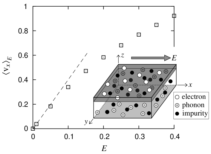
Figure 1: Average of electron velocity in the $x$-direction, plotted against $E$. The dashed line represents the slope of the linear response. Inset: schematic diagram of the simulation system. Electrons are confined in a 2D plane (dark gray). Under the 2D electron system there is a three-dimensional phonon system, the bottom of which is a thermal wall (light gray). Impurities are distributed throughout all regions of the system. An external electric field $E$ is applied in the $x$-direction.

This model is an extension of the two-dimensional model for the MD simulation of electrical conduction, which has been previously proposed in Ref. YIS . A possible experimental situation corresponding to the model in Ref. YIS occurs when the edges of a 2D electron system are in contact with large sample holders (which have large heat capacity and good heat conduction). On the other hand, the present model is a reflection of a typical experimental setup of a quasi-2D electron system in a semiconductor device. That is, a 2D electron system is realized around the top of a bulk substrate (which is modeled by the 3D system of phonons and impurities) and the substrate is mounted on a large sample holder (which is modeled by the thermal wall). The present model is macroscopically uniform in the $y$-direction as well as in the $x$-direction, whereas the previous one was uniform only in the direction parallel to $E$. This enables us to investigate bulk properties in both the $x$- and $y$-directions. It should also be noted that this model is isotropic in the $y$-direction and the net currents of particles and energy in this direction are absent on average.

In Fig. 1 we show $E$-dependence of the average electron velocity $\langle v_{x}\rangle_{E}$ in the $x$-direction. Here $\langle\cdots\rangle_{E}$ denotes the average in the steady state for $E$. A linear response is observed in the regime of small $E$ and a nonlinear response in the regime of large $E$.

Deviation from LEDF. Because of the macroscopic spatial uniformity of the model, steady states in the model are also uniform. That is, local quantities such as local number densities and local kinetic temperatures in steady states are almost independent of the position in the 2D electron plane. We may therefore use electrons in the entire region of the plane to calculate a VDF of electrons. In this paper we investigate distribution functions $P_{y}(v_{y})$ of electron velocity $v_{y}$ in the $y$-direction. [The corresponding results in the $x$-direction (parallel to $E$) will be presented elsewhere YS_dist_x ; these have more complicated structures and properties than those of $P_{y}$ presented here.] In Fig. 2 we show semi-logarithmic plots of $P_{y}$, plotted against $v_{y}{}^{2}$. The data for positive $v_{y}$ almost completely overlap with those for negative $v_{y}$ in NESSs ($E=0.1$ and $0.4$), as well as in the equilibrium state ($E=0$). This indicates that $P_{y}(v_{y})$ is symmetric at $v_{y}=0$, and is consistent with $\langle v_{y}\rangle_{E}=0$, even in the nonlinear response regime. These results are due to the isotropy in the $y$-direction of the model.

Figure 2: (Color online) A semi-logarithmic plot of the distribution $P_{y}$, plotted against $v_{y}{}^{2}$. The results for $E=0$, $0.1$, and $0.4$ are shown. The data for $v_{y}>0$ and $v_{y}<0$ are overlapped. The dashed lines represent the LEDFs $f_{y}^{\rm loc}$. The solid lines depict fitting curves of Eq. (4) for $E=0.1$ and $0.4$. Inset: deviation $P_{y}(v_{y})-f_{y}^{\rm loc}(v_{y})$ from the LEDF. Also shown are the fitting curves of Eq. (4), with $f_{y}^{\rm loc}$ subtracted, for $E=0.1$ and $0.4$ (solid curves).

As an LEDF in the $y$-direction, we employ a naive distribution function defined by

$$f_{y}^{\rm loc}(v_{y})=\sqrt{m_{e}/2\pi T_{e}^{y}}\exp\left(-m_{e}v_{y}^{2}/2T_{e}^{y}\right),$$ (1)

where $T_{e}^{y}=m_{e}\langle v_{y}{}^{2}\rangle_{E}$ is a kinetic temperature in this direction (this is simply a Maxwell distribution with temperature $T_{e}^{y}$). In Fig. 2 we also plot $f_{y}^{\rm loc}$ (in this plot zero-mean Gaussian distributions are drawn as straight lines). We observe that the tails of $P_{y}$ and $f_{y}^{\rm loc}$ are different for large values of $E$, whereas they are almost the same for $E=0$. Moreover in the inset of Fig. 2, we plot the deviation $P_{y}(v_{y})-f_{y}^{\rm loc}(v_{y})$. From this figure we see that the difference around $v_{y}=0$ is also large in the NESSs. The symmetric behavior of the deviation is again consistent with the isotropic nature of the model.

Explicit form of $P_{y}$. To explore the functional form of $P_{y}$ we next investigate a $v_{y}$-dependent “reciprocal temperature”, $\beta_{y}(v_{y})$, which is defined by

$$\beta_{y}(v_{y})=-\frac{2\ln\left[P_{y}(v_{y})/P_{y}(0)\right]}{m_{e}v_{y}{}^{2}}.$$ (2)

If $P_{y}$ is a Maxwell distribution, $\beta_{y}$ is independent of $v_{y}$ and is equal to the reciprocal temperature of the Maxwell distribution. In Fig. 3 we show $v_{y}$-dependence of $\beta_{y}$. Figure 3 (a) is a result for the equilibrium state ($E=0$). In this case $\beta_{y}$ is almost independent of $v_{y}$ and is nearly equal to the reciprocal temperature $1/T_{0}$ ($=1$) of the thermal wall within the precision of the numerical simulation. This is consistent with the fact that in an equilibrium state, $P_{y}$ is a Maxwell distribution with $T_{0}$. Although the data fluctuations are rather large for $v_{y}$’s close to zero and in the tails, they are simply due to the restricted accuracy of the numerical simulation in these regions and they can be expected to become smaller as we average over greater numbers of simulation samples.

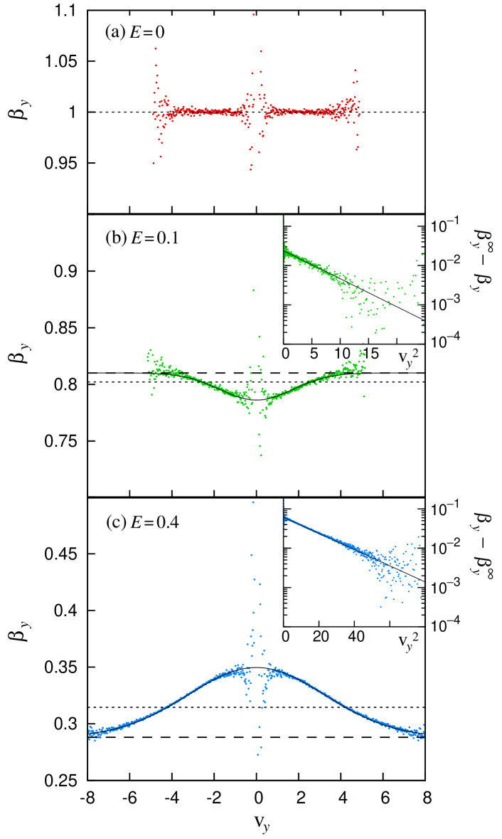
Figure 3: (Color online) Mains: $\beta_{y}$ for (a) $E=0$, (b) $E=0.1$, and (c) $E=0.4$, plotted against $v_{y}$. The dotted and dashed lines represent $1/T_{e}^{y}$ and $\beta_{y}^{\infty}$, respectively ($1/T_{e}^{y}\simeq\beta_{y}^{\infty}\simeq 1/T_{0}=1$ when $E=0$). The solid lines are fitting curves of Eq. (3). Insets: semi-logarithmic plots of (b) $\beta_{y}^{\infty}-\beta_{y}$ and (c) $\beta_{y}-\beta_{y}^{\infty}$, respectively, plotted against $v_{y}{}^{2}$. The data for $v_{y}>0$ and $v_{y}<0$ are overlapped. The solid straight lines represent fitting curves of Eq. (3) (subtracted from $\beta_{y}^{\infty}$ in (b) and reduced by $\beta_{y}^{\infty}$ in (c), respectively).

Figures 3 (b) and (c) show the results for NESSs ($E=0.1$ and $0.4$, respectively). As $|v_{y}|$ becomes large, $\beta_{y}$ varies (increasing in (b) and decreasing in (c)) monotonically and tends to converge to a certain constant value $\beta_{y}^{\infty}$, which is different from both $1/T_{0}$ and $1/T_{e}^{y}$. This implies that $P_{y}$ approaches a Maxwell distribution as $|v_{y}|\to\infty$. Furthermore, we find that the overall behavior of $\beta_{y}$ is well described by a Gaussian function. That is, $\beta_{y}$ is well fitted by

$$\beta_{y}(v_{y})=B\exp(-Dv_{y}{}^{2})+\beta_{y}^{\infty},$$ (3)

where $\beta_{y}^{\infty}$, $B$, and $D$ are fitting parameters. In the insets of Figs. 3 (b) and (c), to see this more clearly, we show semi-logarithmic plots of $|\beta_{y}-\beta_{y}^{\infty}|$ versus $v_{y}{}^{2}$. We observe exponential decay behavior of $|\beta_{y}-\beta_{y}^{\infty}|$ as functions of $v_{y}{}^{2}$, which indicates that the variation of $|\beta_{y}-\beta_{y}^{\infty}|$ is almost equivalent to that of Gaussian functions of $v_{y}$. Although the data for $v_{y}$’s close to zero and in the tails fluctuate rather violently, they would converge to a single curve as the number of samples increases. From Eqs. (2) and (3) we thus obtain an explicit functional form of $P_{y}$ as

$$P_{y}(v_{y})=P_{y}(0)\exp\left[-\left(\beta_{y}^{\infty}+Be^{-Dv_{y}{}^{2}}\right)\frac{m_{e}v_{y}{}^{2}}{2}\right].$$ (4)

This is a main result of the present paper. In Fig. 2 we plot curves of Eq. (4) for $E=0.1$ and $0.4$ as solid lines. These also reveal that Eq. (4) is a good fitting function of $P_{y}$ for almost all values of $v_{y}$.

$E$-dependence. Figure 4 shows the $E$-dependences of parameters in Eq. (4). In the top of Fig. 4 we compare $\beta_{y}^{\infty}$ and $1/T_{e}^{y}$. Although $E$-dependences of these two quantities are similar, their detailed values are different. $\beta_{y}^{\infty}>1/T_{e}^{y}$ at small values of $E$ (as can be seen also in Fig. 3 (b)), whereas $\beta_{y}^{\infty}<1/T_{e}^{y}$ at large values of $E$ (as is seen also in Fig. 3 (c)). In the bottom of Fig. 4 we show the result for $B$. There exists a value $E_{c}$ of the electric field such that $B<0$ if $0<E<E_{c}$ and $B>0$ if $E>E_{c}$ ($E_{c}\simeq 0.15$ in the parameter values of the present simulation). This is consistent with the result for $\beta_{y}^{\infty}$, which is mentioned above. That is, $\beta_{y}^{\infty}>1/T_{e}^{y}$ if $0<E<E_{c}$ and $\beta_{y}^{\infty}<1/T_{e}^{y}$ if $E>E_{c}$.

Figure 4: Top: $E$-dependence of $\beta_{y}^{\infty}$ (circles) and $1/T_{e}^{y}$ (triangles). Bottom: $E$-dependence of $B$.

Summary and discussion. In this paper we have introduced a model of a two dimensional classical electron system which is macroscopically uniform. In the model with an external driving force (electric field $E$), a spatially uniform nonequilibrium steady state (NESS) is realized. By using molecular dynamics simulations we have investigated the distribution function $P_{y}(v_{y})$ of an electron velocity $v_{y}$ in a direction perpendicular to $E$ in a steady state. When the driving force is large, the local equilibrium (LE) description is not valid. We have determined an explicit form of the velocity distribution function (VDF) as Eq. (4), which is valid up to numerical accuracy, even for NESSs where the LE description breaks down. The functional form has a velocity-dependent “reciprocal temperature” $\beta_{y}(v_{y})$. In the limit of large absolute values of $v_{y}$, this reciprocal temperature converges to a constant value $\beta_{y}^{\infty}$, which is different from both the equilibrium temperature and the kinetic temperature, and the VDF thus approaches asymptotically a Maxwell distribution with temperature $1/\beta_{y}^{\infty}$. We have also found that there exists a crossing value of the driving force below (above) which $\beta_{y}^{\infty}>\beta_{y}(0)$ ($\beta_{y}^{\infty}<\beta_{y}(0)$). It might be difficult to obtain such a nontrivial dependence of $\beta_{y}$ on $E$ by a naive perturbation expansion in terms of $E$.

The asymptotic property of the tails of the VDFs in NESSs is similar to that of nonequilibrium distribution functions of microscopic energy currents in thermal conduction models Yukawa_et_al . In those models the distribution function of energy currents parallel to the temperature gradient has a tail for large negative (positive) values of the current which asymptotically obeys an equilibrium distribution with temperature $T_{-}$ ($T_{+}$). Here, $T_{-}$ and $T_{+}$ are different from the local temperature at the place where the distribution is measured, but equal to the local kinetic temperatures at slightly forward and backward regions, respectively. In the present model of electrical conduction, the tails of the VDF asymptotically obey an equilibrium distribution with temperature $1/\beta_{y}^{\infty}$. Although $1/\beta_{y}^{\infty}$ is equivalent in the tails for positive and negative values of velocity (because of the isotropy of the model in the direction perpendicular to the driving force), it differs from both the equilibrium temperature and the kinetic temperature. We therefore expect that it is a universal feature in NESSs that the distribution function of a microscopic current approaches an equilibrium distribution in the limit of large currents. This might be related to a representation of the nonequilibrium distribution of microscopic states, which has been derived recently KNST .

Unlike the results for thermal conduction models, we do not yet know the physical meaning of the temperature $1/\beta_{y}^{\infty}$. Also we do not understand the meanings of other parameters in the functional form of the VDF and the crossing value of the driving force. These subjects remain for future research.

The author is grateful to A. Shimizu for helpful discussions and comments.

References

- (1) Kim. H.-D. and H. Hayakawa, J. Phys. Soc. Jpn. 72, 1904 (2003), and references cited therein.
- (2) W. Loose and S. Hess, Phys. Rev. Lett. 58, 2443 (1987).
- (3) K. Aoki and D. Kusnezov, Phys. Rev. E 70, 051203 (2004).
- (4) A. Ueda and S. Takesue, J. Phys. Soc. Jpn. 75, 044003 (2006).
- (5) S. Yukawa, T. Shimada, F. Ogushi, and N. Ito, J. Phys. Soc. Jpn. 78, 023002 (2009).
- (6) T. Yuge, N. Ito, and A. Shimizu, J. Phys. Soc. Jpn. 74, 1895 (2005).
- (7) T. Yuge and A. Shimizu, in preparation.
- (8) T. S. Komatsu, N. Nakagawa, S. Sasa, and H. Tasaki, J. Stat. Phys. 134, 401 (2009).